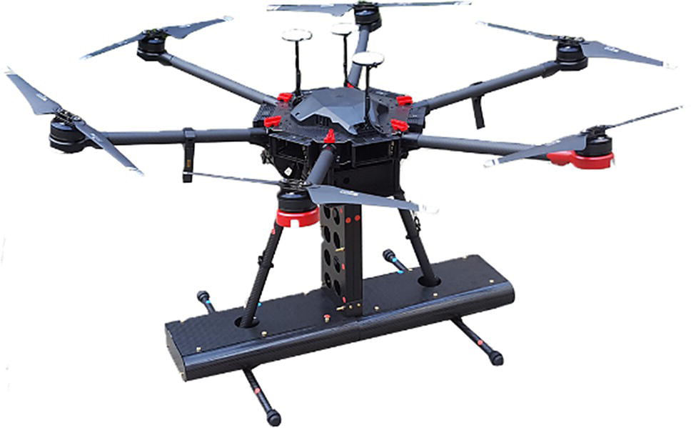
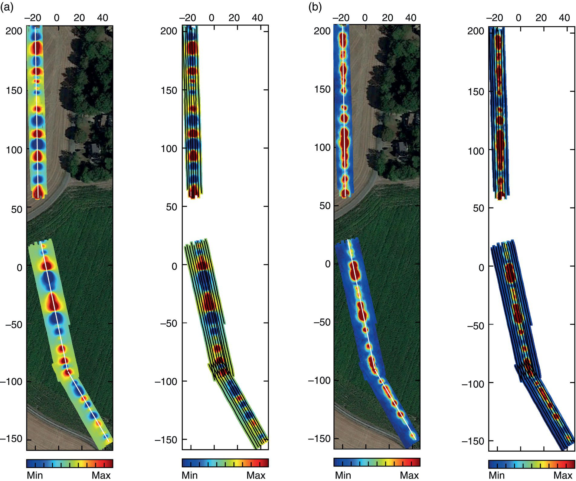
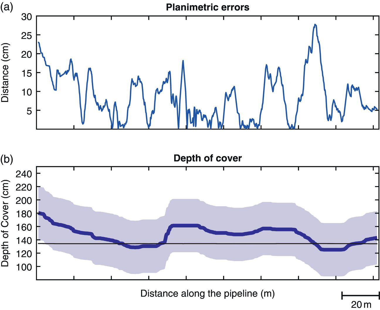
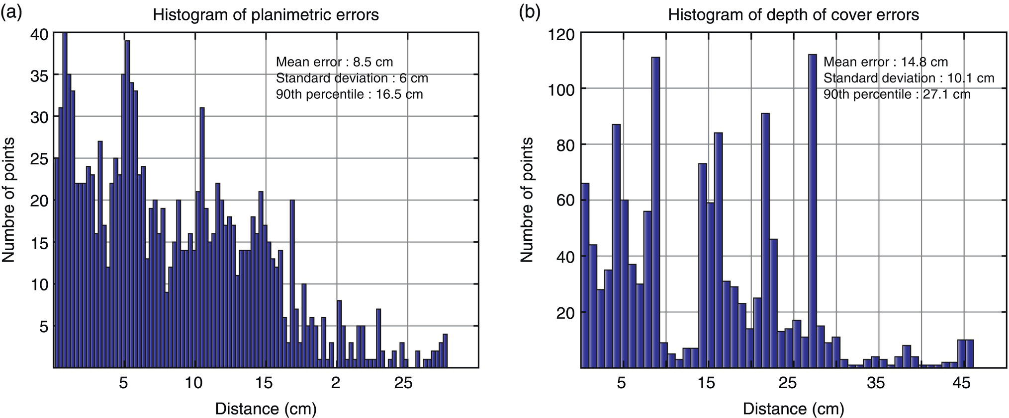
Mehdi M. Laichoubi1, Hamza Kella Bennani1, Ludovic Berthelot1, Vincent Benet1, Miaohang Hu1, Michel Pinet2 and Samir Takillah1 1Skipper NDT, R&D Department, Paris, France 2GRTgaz, Technical Direction, Paris, France Pipeline incidents related to third-party work around the world reached a peak in 2022. About 30% of reported incidents were due to poor pipeline geolocalization [1]. The integrity of pipeline networks is also at risk due to increased encroachment because of urbanization. As a result, some governments enforce stringent rules on pipeline operators concerning their network georeferencing. The currently available tools to position and assess the depth of cover (DOC), which use electromagnetic or ground-penetrating radar (GPR) technologies, are handheld and particularly challenged in remote rural locations, where constraints are related to the safety of field operators, specific soil and culture conditions. UAS are often deployed in difficult-to-access locations as they present significant operational advantages in terms of operators’ safety, speed of execution, cost-efficiency, and access to impracticable terrains. Currently available technologies focus on above-ground measurements through various methods, such as thermal and hyperspectral imaging or light detection and ranging (LiDAR). A proprietary embedded system and acquisition protocol have been developed that combine the advantages of a drone vector and high precision magnetometry. The technology makes it possible to obtain information about the magnetic underground environment of the pipeline as well as an accurate and continuous 3D localization (longitude, latitude, and DOC). The accuracy and data density achievable with this method unlock strain assessment capabilities that are particularly relevant regarding the threats of pipeline infrastructure from weather and outside forces (WOF). WOF has continued to gain the attention of both operators and regulators, primarily due to the growing threat of geohazards and the increasing number of public incidents. An extensive series of field trials conducted in France with Europe’s leading gas pipeline operator, GRTgaz, are discussed in this chapter, including the qualification of the georeferencing performance of the technology in the highest precision category (Class A, according to the French regulation), under various operational conditions. A case study in comparison with the in line inspection (ILI) tool is also discussed regarding strain assessment capabilities. Buried pipelines have been used for many years and will continue to be used for many years to transport oil, gas, and water. Addressing the challenge of third-party damage to this critical infrastructure is a pressing issue for operators and regulators. Some countries have started to enforce stringent legal requirements. In France, a government decree mandates operators to map critical pipelines, at least at 40 cm precision, both in planimetry (X, Y) and in altimetry (Z) for 90% of the measured points. It corresponds to the class A precision detailed in the NF S70-003 AFNOR standard [2]. Geolocalization of pipelines can be achieved using different technologies on an open or closed ditch. The focus here is on geolocalization of pipelines in a closed ditch, which is traditionally and mainly done using electromagnetic field (EMF) measurements with handheld receivers [3–6] and GPR techniques. Operationally, these measurements require an operator carrying or pushing the measuring device along the right-of-way (ROW). Based on the previous research of Laichoubi et al. [7] involving acquisition and processing of magnetic maps as a method for pipeline 3D-geolocalization, it has been proposed to record the magnetic field components along with geopositioning data on a pipeline ROW to determine the horizontal location of the pipe and the depth below ground level with a precision level corresponding to the class A requirements. In recent years, technological advances have been made in the integration of remote sensing and magnetic measurement systems for unmanned aerial systems (UAS), which makes it possible to perform a survey without involving operators on the ROW. Table 25.1 Summary of Eight GRTgaz Pipeline Spot Inspections under Various Operational Configurations In this chapter, several trials conducted jointly with GRTgaz (France) in 2021 are discussed. In order to demonstrate this proof-of-concept study, eight pipeline locations with different diameters ranging from 80 to 1200 mm (3–48 in.) were selected by GRTgaz. It took 5 h of cumulative flight time for a 2.7 km inspected distance. Table 25.1 illustrates the performance of this innovation and the accuracy of georeferencing in class A. The analysis and methodology are illustrated on an 8-in. (200 mm) diameter pipeline with: (1) total magnetic intensity maps, (2) comparison of the geolocation data from this magnetic technology with a land surveyor reference, and (3) the error histograms in planimetry and depth. The hardware developed consists of a 4.2 kg and a 90 cm wide embedded system that can be mounted under a UAS (Figure 25.1). The main components of the device are: (1) five three-components fluxgate magnetometers; (2) a real-time global navigation satellite system GNSS receiver with a centimetric-level precision; (3) a tactical grade inertial measurement unit (IMU); (4) a remote sensor measuring the distance between the magnetometers and the ground (or canopy); and (5) a proprietary electronic card for data acquisition, digitalization, and synchronization. Figure 25.1 The embedded system mounted under an off-the-shelf UAS. (Gautam et al. 2018/MDPI/CC BY 4.0.) The main sensors in this system are the magnetometers and the GNSS, upon which the acquisition of the magnetic map depends. The fluxgate magnetometers measure the three components of the magnetic field at a 1000-Hz sample frequency for 112 g mass per unit. Compared to scalar magnetometers, fluxgate magnetometers are more suited to UAS constraints with overall lighter, more robust sensors with a ten to hundred times higher sampling frequency. Even if the fluxgate magnetometer has a lower resolution/precision, it is sufficient for the nanoTesla to microTesla range of magnitude that is required. The other point to be considered is that, compared to scalar magnetometers, fluxgate magnetometers are used to measure the components of the magnetic field, allowing compensation of the magnetic effect of the embedded equipment and UAS. Thus, the system can be adapted to different vectors without any custom characterization. This subject is not new and was developed in the 1970s for magnetic compensation of airplanes in airborne geophysics [8, 9]. On the other hand, because fluxgate magnetometers are not absolute instruments with inherent errors of offset, sensitivity, and angle (nonorthogonality), they must be calibrated. In our context, GNSS hardware needs to face stringent precision and weight constraints. On the other hand, lightweight GNSS hardware is commonly used for UAS applications, a 606 g receiver and antenna system offering more technical capabilities were chosen. Multifrequency and multi-GNSS hardware is used for real-time precise point positioning (PPP) correction services. The corrections ensure positioning accuracies down to ±4 cm at 95% root-mean-square worldwide (between –75° and +75° latitude). This precision can be reached without deploying a base station on the field and without the need for an internet connection, facilitating operations and logistics. Other components of the system serve mainly a corrective purpose. Indeed, contrary to ground-based systems, flying equipment requires supplementary corrections. The IMU is used to perform level control to correct the navigation in case of heading misalignment with the route. The level control can also be used for the change of reference frame for the measured magnetic components [10]. The remote sensor combines measurements from ultrasonic and LiDAR to evaluate the distance from the magnetometers and the ground or canopy and then infer the depth of the pipeline below ground. Obtaining the total magnetic intensity map follows a four-step protocol, described in the following paragraphs, on a real case study on the ROW of a GRTgaz buried pipeline. Parallel magnetic profiles are acquired on an 8-inch diameter gas pipeline over 400 m. The data are processed as follows to obtain the total magnetic intensity map: (1) calibration parameters are used to calibrate the data, as shown by Munschy et al. [11], where both calibration and compensation are applied using the same kind of function (Figure 25.2); (2) the start and end of each profile are identified; (3) the data are edited to check for spikes; (4) the total magnetic intensity map is computed by interpolation of data profiles. More often the node spacing of the magnetic map is 0.2 m. The total magnetic intensity map and related analytic signal are then used to locate the pipeline by computing its horizontal location and depth below the ground. The magnetic map shown in Figure 25.3a was obtained using the UAS-embedded magnetic device described above. This map results from the acquisition of 7–10 profiles per flight, spaced by 1.5 m, over 3 flights, with the 5 sensors 2 m above ground level for each flight. The map mainly shows the alignment of magnetic anomalies due to the pipe sections with an amplitude of about 3000 nT. The spatial derivatives of the magnetic map are computed and used to determine the analytic signal shown in Figure 25.3b. Profiles orthogonal to the pipeline direction are extracted from the magnetic maps using the full 500-Hz exploitable magnetic spectrum to determine the horizontal position and depth under the ground of the considered line [7]. The objective of this study was to evaluate the capabilities of the UAS magnetic mapping method to localize a pipeline within the highest positioning thresholds defined by the French regulation for rigid buried facilities: class A. This benchmark is detailed in the standard NF S70-003-3 with three planimetric error thresholds and two altimetric/depth error thresholds. It can be summarized by one threshold for both planimetric positioning and depth positioning errors of 40 cm for 90% of the measured points on a line. Figure 25.2 Example of calibration results for one of the five magnetic sensors. (a) The two curves correspond to the noncalibrated (black line, standard deviation 85.1 nT) and calibrated (grey line, standard deviation 1.7 nT) intensities of the magnetic field measured by the fluxgate sensor. The green curve is the intensity of the Earth’s magnetic field at the location of the calibration, (b) the nine estimated calibration parameters and their standard deviations. Figure 25.3 (a) Total magnetic intensity map with estimated positioning (x, y) of the buried pipeline (white line, left panel). The UAS trajectory that generated this map is indicated by black lines, (b) analytical signal map with estimated positioning (x, y) of the buried pipeline (white line, left panel). The trajectory of the UAS that generated this map is indicated by black lines. All maps are displayed considering the x-axis as distance east and the y-axis as distance north. To establish the error histograms on our 8-in. pipeline case study, we compared our 3D localization using UAS magnetic mapping to a reference line measured by a land surveyor using traditional methods. The focus is the 183-m south section of the line including a bend to estimate the relative errors (i.e., differences between locations identified using UAS magnetic mapping and the locations measured by a land surveyor), as illustrated in Figure 25.4. The planimetric error shown in Figure 25.4a is mainly under the 20 cm line with a maximum of 28 cm. The error histogram shown in Figure 25.5a is compliant with class A requirements in terms of planimetry. The variations around the reference line may be explained by the cumulative errors of each system, and neighbor the measurement uncertainties of the reference line positioning are approximated. The depth error is presented with a ±20 cm error halo that encompasses the black reference line everywhere but in the first few meters. The error histogram shown in Figure 25.5b is also compliant with class A requirements in terms of depth below ground with a maximum error of 47 cm in the first meter of inspection. The change of topography during the 11 months between the time that the magnetic map was acquired and the time that the reference line was established may explain the fact that the histogram of depth errors does not follow a folded normal distribution. Ultimately, the pipeline was successfully positioned within the requirements of class A by the system in 36 min of cumulative total flight time. Figure 25.4 Estimation of error relative to the reference line. (a) Planimetric errors relative to the reference line, (b) depth of cover relative to the reference line. Figure 25.5 Histograms of distance error in geolocalization by SKIPPER NDT to the reference line. (a) Histogram of the planimetric error to reference line and its mean, standard deviation, and 90th percentile, (b) Histogram of the depth of cover error to the reference line and its mean, standard deviation, and 90th percentile. The same protocol was repeated on an extensive set of eight pipelines with different diameters and ROW conditions for a total distance of 2.7 km. The test sessions included inspection near railways, under high-voltage lines, with the presence of concrete protections, and on steep terrains and wheat fields. In Table 25.1, the valid inspected distance represents the inspected areas compliant with the requirements of our technology, which excludes areas where the ROW is too narrow to get the full magnetic anomaly, areas of poor GNSS coverage, or simply areas where the flights were prohibited, such as construction sites, and roads. The percentage of class A corresponds to the ratio between the distance successfully geolocalized within A class planimetric requirements and the valid inspected distance. The threat from WOF is becoming a priority for operators and regulators, due to the increasing threat of geohazards and the growing number of public incidents, mainly associated with girth weld failures. Currently, geohazard threats are essentially identified by aerial reconnaissance, foot patrols, LiDAR, and bending strain assessments based on data gathered from IMU incorporated onto in-line inspection tools. Each of these methods has some limitations that include the timeline of results, accessibility requirements, or ability to characterize the pipe response. Incidents related to geohazards often create high-profile situations where the pipeline ROW has been visibly disrupted (i.e., landslides), but the condition of the pipeline is unknown. A rapid response technology capable of providing an assessment of the pipe’s total strain condition offers significant benefits to the pipeline industry. A high-resolution drone-based bending strain (DBBS) assessment has been developed, relying on magnetic mapping of the ROW. It uses the magnetic field of the pipeline and proprietary processing algorithms to determine the position of the pipe. The system shows comparable performance to ILI methods and is highly competitive in terms of cost and time of operation. The DBBS intervenes on the same level as the ILI in the chart (Figure 25.6); it does not explicitly measure the bending strain in the pipeline. Rather, the premise of the technology is that it accurately determines line location and relative deflection from a straight line in a manner that is similar to walking along the pipeline above ground with a line locator. This information can then be used to estimate the bending strain according to the previously published methods [12]. As Fathi et al. [13] have shown, relatively simple pipeline location data produced using conventional pipeline location and surveying equipment can be used to estimate total longitudinal strain demand (incorporating axial and bending strain) resulting from pipeline deflection caused by a geohazard. Thus, a DBBS solution may be considered to deliver a quick and cost-efficient preliminary answer where ILI is not yet required, or simply on unpiggable lines. It has been compared to the gold standard ILI method to evaluate its relevance. Figure 25.6 Chart showing the methods to assess ground-induced deformations on buried pipelines, with DBBS and ILI methods. A case study has been conducted to compare the positioning, the out-of-straightness (OOS), and the strain estimation on intentional bends over 500 m on 24″ diameter pipelines. Localization results are very close to the ILI results (see Table 25.2), which leads to good OOS estimation for the filtered and smoothed data. The technology was able to pick up direction changes as small as 2.5° in azimuth and 1.5° in pitch. Nevertheless, strain evaluation is not efficient since it was not able to match any of the spikes present in the ILI results (Figure 25.7). The main issue about deriving the pitch and Azimuth into understandable strain is the signal over noise ratio that needs to be managed. The DBBS introduces more noise in its position measurement than the IMU for an ILI. This impacts especially the detection of short bends like cold bends here. The focus has been on a filtering method to clean up the noise in the signal without compromising valuable information. This filtering method was then applied at different steps of the strain calculation process to come up with a better strain evaluation on bends, presented in Figures 25.8 and 25.9. On these figures, the focus was on strain evaluation around the area of interest with a threshold of 0.2% for bends. In this use case, compensation for the noise was successful without compromising the signal. The outcome can be summarized in a confusion matrix (Tables 25.3 and 25.4) Table 25.2 Horizontal and Vertical mean and Max Positioning Error between DBBS and ILI Methods The new filtering method improved the true positive rate on both vertical and horizontal strains. It has drastically reduced the false negative by keeping the false positive at zero. Regarding the vertical strain, the true positive/false negative could easily go to 3/1 considering the proximity of the spike at 120 m shown in Figure 25.6. Nevertheless, all detected bends have an underestimated strain value using DBBS. Table 25.5 tends to show that horizontal strain is underestimated by 26% and vertical strain is underestimated by 50%. This study demonstrates successful trials conducted with Skipper NDT and GRTgaz. 89% of the valid inspected distance was georeferenced in class A on various pipeline configurations, ROW, and diameters. Skipper NDT technology and results were validated by GRTgaz which makes the system approved for use by land surveyors for the rural geolocalization campaign AcaPulCO 2. The UAS embedded system for magnetic mapping proved that it was affected by neither high voltage lines and railways interferences nor crops and soil conditions on the ROW. The DBBS assessment compared to the gold standard (ILI) shows great results in terms of positioning and OOS assessment. After adapted filtering of the signal, the strain curves on the case study matches the ILI curves for both horizontal and vertical strains. Despite the great detection performances, strain values are underestimated and more specifically on the vertical axis by a constant factor. It should be mentioned that these results were obtained after 40 min of cumulative flight time and without any interruption of the pipeline flow. The method still requires some improvements:—Refine the filtering to find the best parameters if a unique set exists. If not, find a method to adapt the filtering to each case;—Enhance the vertical strain estimation by improving the vertical positioning. This issue is most certainly due to GNSS capabilities that are typically better in XY positioning. GNSS convergence time and the PPP capabilities were challenged in several locations that make areas near forests difficult to inspect. This issue is now solved by postprocessed kinematic (PPK) differential correction (by recovering the satellite’s ephemeris at day+1) using base stations (public or private) on georeferenced points. This solution presents limitations, such as flight authorizations and obstructed ROW. Indeed, the ROW needs to be free from obstacles 2m or higher for a 10-m width and present a uniform elevation in the line’s perpendicular direction. The geolocalization on 90° bends for large pipelines, 750 mm diameter (30 in.) and higher, tends to follow the exterior of the elbow causing a mispositioning which explains the results for the 900 mm (36 in.) and 1200 mm (48 in.) diameter pipelines given in Table 25.1. Ferromagnetic parallel lines under 5 m distance have an impact on the positioning performance, especially if they are electrically connected. All these aspects are considered for an ongoing R&D program. Figure 25.7 Six-panel DBBS versus ILI comparison of horizontal/vertical OOS (in meters), pitch/azimuth (in degree), and horizontal/vertical bending strain (in %). Figure 25.8 Horizontal strain (%) comparison between the ILI (solid line) and the DBBS (line marked with stars). Figure 25.9 Vertical strain (%) comparison between the ILI (solid line) and the DBBS (line marked with stars). Table 25.3 DBBS Detection Performance Comparing Old and New Filtering Methods for Horizontal Strain Table 25.4 DBBS Detection Performance Comparing Old and New Filtering Methods for Vertical Strain Table 25.5 DBBS Underestimation with Respect to the ILI Strain Reference for Each True Positive Detection for both Horizontal and Vertical Strains, ΔStrain is the Difference Between the Two Methods The technology is currently available for geolocalization applications as a tool for difficult-to-access and complex locations. Moreover, the technology may also be applied at river crossings and for OOS assessments.
25
3D-Geolocalization by Magnetometry Using UAS: A Novel Method for Buried Pipeline Mapping and Bending Strain Assessment
25.1 Introduction
25.2 3D Localization and Depth of Cover Assessment
Nominal Pipe Size (mm/in.)
Valid Inspected Distance (m)
Percentage of Class A
Cumulative Flight Times (min)
80/(3)
119
100%
20
100/(4)
335
100%
37
150/(6)
280
100%
18
500/(20)
263
56%
39
600/(24)
387
100%
51
600/(24)
63
100%
17
900/(36)
861
89%
80
1200/(48)
404
64%
37
25.3 Materials and Methods
25.4 Case Study and Operating Procedure
25.5 Performance of the 3D Localization

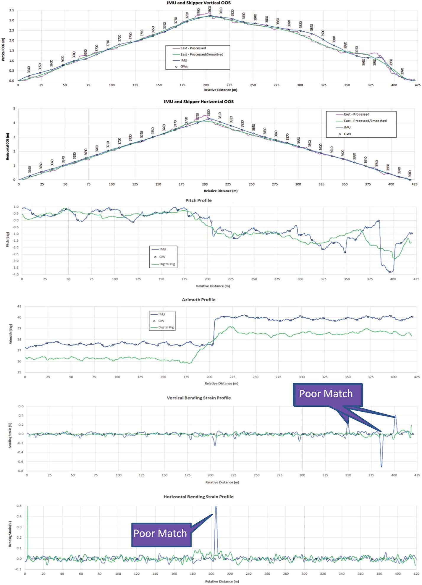
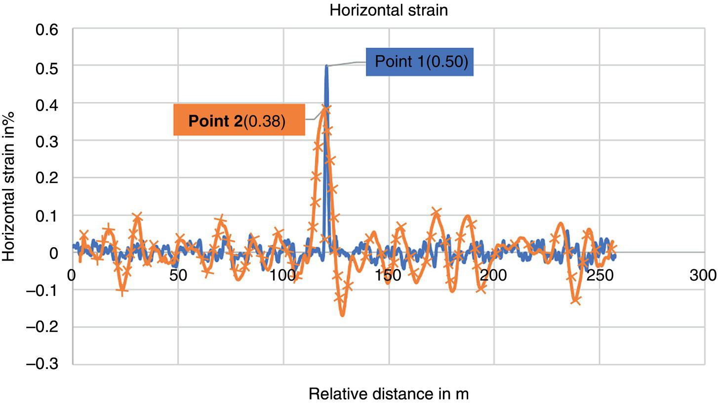
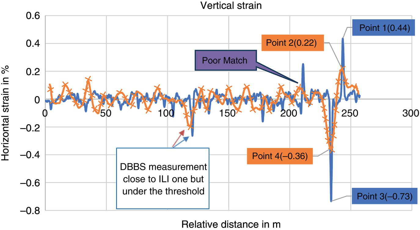
25.6 Generalized Study on Eight GRTgaz Pipeline Spots
25.7 Bending Strain Assessment
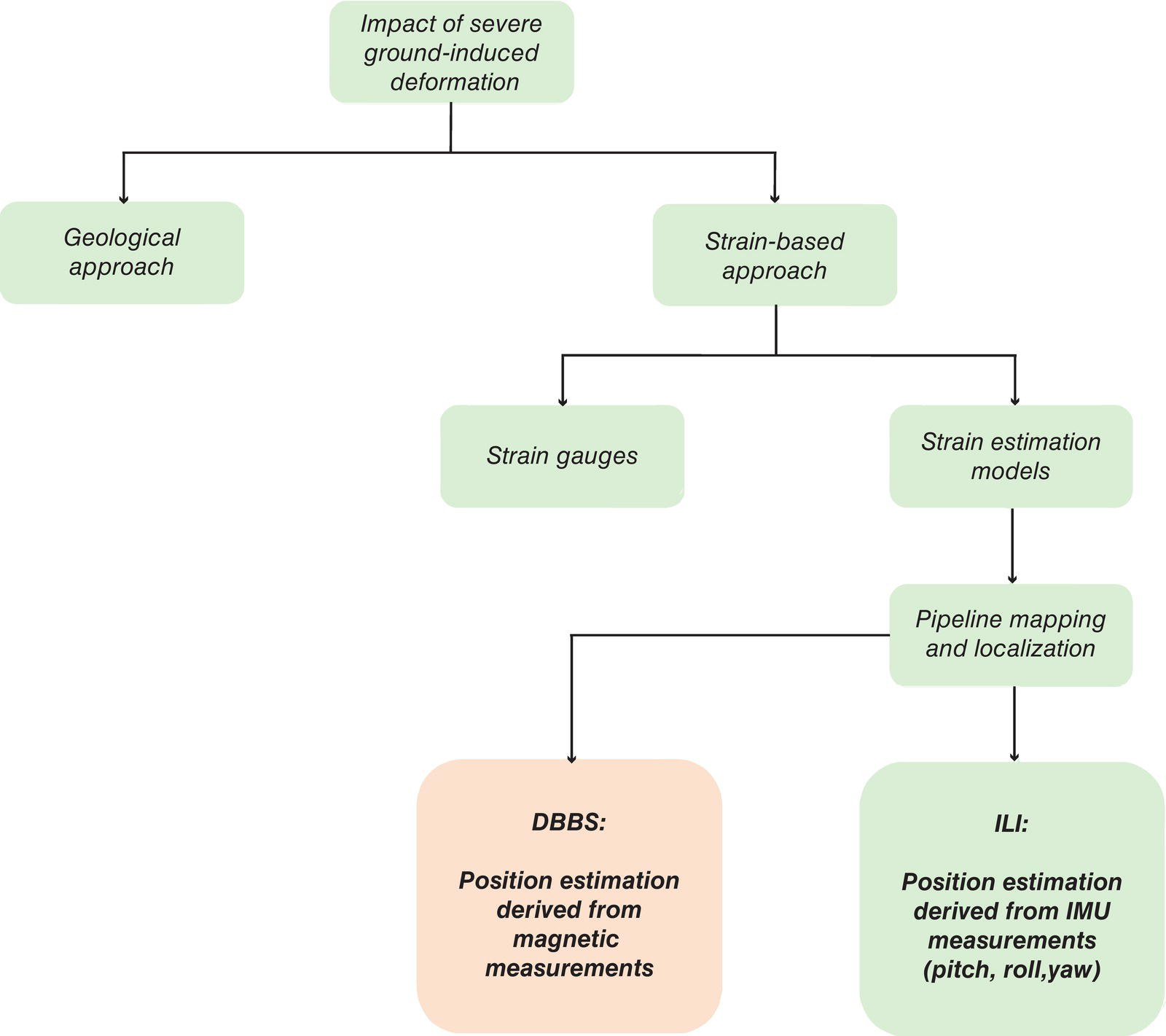
25.8 Drone-Based Bending Strain (DBBS) Case Study
OOS Direction
Mean Error (cm)
Max Error (cm)
Horizontal
6.6
21.8
Vertical
8.5
30.1
25.9 Conclusion
Horizontal Strain
Old Filtering Method
New Filtering Method
True positive
0
1
False positive
0
0
False negative
1
0
Vertical Strain
Old Filtering Method
New Filtering Method
True positive
0
2(3)
False positive
0
0
False negative
4
2(1)
Detection Points
ΔStrain Value
Strain Ratio
Horizontal
Point 1-2
0.12%
0.76
Vertical
Point 1-2
0.22%
0.5
Point 3-4
0.37%
0.49
References