RESUMING where we left off in Chapter 2, if we had the phase-space probability density ρ(p,q), we could calculate averages of phase-space functions, 〈A〉=∫ΓA(p,q)ρ(p,q)dΓ, Eq. (2.53). For equilibrium systems, ρ(p,q)=F(H(p,q)), Eq. (2.57), where F is an unknown function. In this chapter, we show that F depends on the types of interactions the systems comprising the ensemble have with the environment (see Table 1.1). We distinguish three types of ensemble:
Isolated systems: systems having a well-defined energy and a fixed number of particles. An ensemble of isolated systems is known as the microcanonical ensemble;1
Closed systems: systems that exchange energy with the environment but which have a fixed number of particles. An ensemble of closed systems is known as the canonical ensemble;
Open systems: systems that allow the exchange of matter and energy with the environment. An ensemble of open systems is known as the grand canonical ensemble.
4.1.1 The microcanonical ensemble: Systems of fixed U,V,N
Phase trajectories of N-particle, isolated systems are restricted to a (6N−1)-dimensional hypersurface SE embedded in Γ-space (the surface for which H(p,q)=E). Referring to Fig. 2.5, for M a set of points on SE, the probability P(M) that the phase point lies in M is, using Eq. (2.64),
P(M)=1Ω(E)∫M∩SEdSE‖∇ΓH‖,
(4.1)
where Ω(E)=∫SEdSE/‖∇ΓH‖ is the volume2 of SE, Eq. (2.64). The expectation value of a phase-space function ϕ(p,q) is, using Eq. (2.65),
where we’ve used the property of the Dirac delta function, that for a function g:ℝN→ℝ, ∫ℝNδ(g(r))f(r)dNr=∫g−1(0)dσf(r)/‖∇g‖, where dσ is the volume element of the (N−1)-dimensional surface specified by g−1(0). The phase-space probability density for the microcanonical ensemble, the microcanonical distribution, is, from Eq. (4.2),
ρ(p,q)=1Ω(E)δE−H(p,q).
(4.3)
Equation (4.3) indicates for an ensemble of isolated systems each having energy E, that a point (p,q) in Γ-space has probability zero of being on SE unless H(p,q)=E, and, if H(p,q)=E is satisfied, ρ(p,q) is independent of position on SE.
We’re guided by the requirement that ensemble averages stand in correspondence with elements of the thermodynamic theory (Section 2.5). In that way, the macroscopic behavior of systems is an outcome of the microscopic dynamics of its components. The consistency of the statistical theory with thermodynamics is established in Section 4.1.8. Thermodynamic relations in each of the ensembles are most naturally governed by the thermodynamic potential having the same variables that define the ensemble. The Helmholtz energy F=F(T,V,N) is the appropriate potential for the closed systems of the canonical ensemble (Section 4.1.9), and the grand potential Φ=Φ(T,V,μ) is appropriate for the open systems of the grand canonical ensemble (Section 4.1.3). We’ll see that the normalization factor on the probability distribution in the canonical ensemble, the canonical partition function Zcan, Eq. (4.53), is related to F by Zcan=exp(−F/kT) (see Eq. (4.57)); likewise in the grand canonical ensemble, the grand partition function ZG, Eq. (4.77), is related to Φ by ZG=exp(−Φ/kT) (see Eq. (4.76)). With that said, which quantity governs thermodynamics in the microcanonical ensemble? Answer: Consider the variables that specify the microcanonical ensemble. Entropy S=S(U,V,N) is that quantity, with Ω=exp(S/k) in Eq. (4.3).
4.1.2 The canonical ensemble: Systems of fixed T,V,N
We now find the Boltzmann-Gibbs distribution, the equilibrium probability density function for an ensemble of closed systems in thermal contact with their surroundings. The derivation is surprisingly involved—readers uninterested in the details could skip to Eq. (4.31).
4.1.2.1The assumption of weak interactions
We take a composite system (system A interacting with its surroundings B; see Fig. 1.9) and consider it an isolated system of total energy E. Let Γ denote its phase space with canonical coordinates {pi,qi}, i=1,⋯,3N, with A having coordinates {pi,qi} for i=1,⋯,3n and B having coordinates {pi,qi} for i=3n+1,⋯,3N, where N≫n. We can write the Hamiltonian of the composite system in the form H(A,B)=HA(A)+HB(B)+V(A,B), where HA(HB) is a function of the canonical coordinates of system A(B), and V(A,B) describes the interactions between A and B involving both sets of coordinates. The energies EA≡HA, EB≡HB far exceed the energy of interaction V(A,B) because EA and EB are proportional to the volumes of A and B, whereas V(A,B) is proportional to the surface area of contact between them (for short-range forces). For macroscopic systems, V(A,B) is negligible in comparison with EA, EB. Thus, we take
E=EA+EB,
(4.4)
the assumption of weak interaction between A and B (even though “no interaction” might seem more apt). We can’t take V(A,B)≡0 because A and B would then be isolated systems. Equilibrium is established and maintained through a continual process of energy transfers between system and environment; taking V(A,B)=0 would exclude that possibility. For systems featuring short-range interatomic forces, we can approximate E≈EA+EB when the surface area of contact between A and B does not increase too rapidly in relation to bulk volume (more than V2/3 is too fast).3 No matter how small in relative terms the energy of interaction V(A,B) might be, it’s required to establish equilibrium between A and B. We’re not concerned (in equilibrium statistical mechanics) with how a system comes to be in equilibrium (in particular how much time is required). We assume that, in equilibrium, EA,EB≫|V(A,B)|, with Eq. (4.4) as a consequence.
4.1.2.2Density of states function for composite systems
The phase volume of the composite system associated with energy E is found from the integral
V(E)=∫{EA<E}dΓA∫{EB<E−EA}dΓB≡∫{EA<E}VB(E−EA)dΓA,
(4.5)
where {EA<E} indicates all points of ΓA for which EA<E, and {EB<E−EA} indicates the points of ΓB for which EB<E−EA. As an example of the integral in Eq. (4.5), suppose one wanted to find the area of the xy-plane for which x+y≤E, where x,y≥0. One would have the integral ∫0<x<Edx∫0<y<E−xdy=∫0Edx(E−x). From Eq. (2.64), dΓA=ΩA(EA)dEA, and thus Eq. (4.5) can be written V(E)=∫0EΩA(EA)VB(E−EA)dEA. Because VB(E−EA)=0 for EA>E, the limit of integration can be extended to infinity:
V(E)=∫0∞ΩA(y)VB(E−y)dy.
(4.6)
By differentiating Eq. (4.6) with respect to E, we have from Eq. (2.64) a composition rule for density-of-state functions when the total energy is conserved and shared between subsystems:
Ω(x)=∫0∞ΩA(y)ΩB(x−y)dy≡ΩA*ΩB.
(4.7)
The density of states function of a composite system Ω is a convolution of the density-of-state functions of the subsystems, ΩA and ΩB.
Example. The density of states function for a free particle in n spatial dimensions, Eq. (2.19), which we denote g(n)(E), satisfies Eq. (4.7),
g(n+m)(E)=∫0Eg(n)(y)g(m)(E−y)dy,
(4.8)
where the limit of integration is finite because g(E−y)=0 for y>E. See Exercise 4.4.
Equation (4.7) generalizes to a system of n subsystems, where xi denotes the energy of the ith subsystem:
Ω(x)=∫0∞∏i=1n−1Ωi(xi)dxiΩnx−∑i=1n−1xi,
(4.9)
where the multiple integration is over the (n−1)-dimensional space for which xi>0. The limits of integration can be extended to infinity because Ωn(y<0)=0. Equation (4.9) is a key result in the development of the theory; it follows by induction from n to n+1 by decomposing Ωn into two components and using Eq. (4.7).
4.1.2.3Probability distribution for subsystems
For an isolated system of energy E consisting of system A together with its environment B, let MA be a set of points in ΓA having canonical coordinates {pi,qi}, i=1,⋯,3n. Let M be a set of points in Γ-space containingMA, such that the first 3n pairs of its canonical coordinates {pk,qk}, k=1,⋯,3N, belong to MA. (In math speak, MA is embedded in M). Thus, phase points having coordinates {pi,qi}, i=1,⋯,3n belong to MA if and only if the phase point of Γ-space belongs to M. The probability that a phase point of A lies in MA coincides with the probability that the phase point of Γ lies in M. Using Eq. (4.1), which pertains to an isolated system,
and we’ve used Eq. (2.65). The final integral in Eq. (4.10) directs us to find the phase volume of M for energies up to and including E. Thus (compare with Eq. (4.5)),
We therefore have, from Eq. (4.12), the phase-space probability density for system A:
ρA(p,q)=ΩB(E−EA)Ω(E),
(4.13)
where EA=HA(p,q). Equation (4.12) implies an energy distribution by setting dΓA=ΩA(EA)dEA. Thus,
ρ(EA)=1Ω(E)ΩA(EA)ΩB(E−EA).
(4.14)
Equations (4.13) and (4.14) are the canonical distribution functions, subsystem probability distributions determined by the density of states functions for the subsystem and the environment.
It might seem that we’re done, but we’re only part way there. These formulas are not in a form we can use for calculations because we lack expressions for the density-of-state functions.4 The interpretation of these formulas is quite physical, however. The probability that system A has energy EA is specified by a ratio of two numbers: the number of states system A has available at energy EA multiplied by the number of states system B has at energy E−EA, to the number of states the composite system has at energy5E. Our strategy in what follows is to develop an expression for Ω(x) appropriate to systems having large numbers of components; see Section 4.1.2.5.
4.1.2.4Partition function: Laplace transform of the density of states function
The canonical distribution requires that we know the density-of-state functions of the system and the surroundings. Density-of-states functions satisfy a convolution relation, Eq. (4.9). By the convolution theorem,6 the integral transform T of a convolution integral is equal to the product of the transforms of the functions appearing in the convolution, T(f*g)=T(f)T(g). The Laplace transform of Ω(x) is known as the partition function:7
Z(α)≡∫0∞e−αxΩ(x)dx,
(4.15)
where α>0. The Laplace transform is the natural choice of transform (as opposed to Fourier) because Ω(x≤0)=0. We’ll soon give α a physical interpretation, but for now we treat it as a mathematical parameter.8
Partition functions obey a simple composition law. By taking the Laplace transform of Eq. (4.9), we find for a system composed of n subsystems ( Zi(α) is the Laplace transform of Ωi(x)),
Z(α)=∏i=1nZi(α),
(4.16)
where the parameter α applies to all subsystems.9 Equation (4.16) implies a useful feature of partition functions. We can consider each molecule of a system as a subsystem! For a gas of N identical molecules, if z(α) is the partition function of a single molecule (Laplace transform of its density of states function), Z(α)=z(α)N.
The partition function is always positive. A positive function Z(α) is log-convex if lnZ(α) is convex (see Section C.1 for the definition of convex function). From Eq. (4.15), Z(α) is log-convex:
In the next subsection, we use the fact that, based on the convexity of lnZ, there is but one solution to the differential equation ( a>0):10
ddαlnZ(α)=Z′(α)Z(α)=−a.
(4.18)
4.1.2.5Density of states function from the central limit theorem
One can devise a probability density having the partition function as its normalizing constant. Define, for α>0,
U(α,x)≡1Z(α)e−αxΩ(x)x>00x≤0.
(4.19)
The functions {U(α,x)} are a family of probability densities (each meets the requirements in Eq. (3.26)), one for each value of α. We’ll single out a member of the family as physically relevant through the requirement that it generate the energy expectation value.11
where the middle equality follows from Eq. (4.15). If we knew Z(α), we would have the first moment of U(α,x), and there is but one solution of Eq. (4.20) for 〈E〉>0. Among the functions U(α,x), there is precisely one that generates a given expectation value. Moreover, the variance of U(α,x) is (see Eq. (3.34))
where we’ve used Eq. (4.17). The first two moments of U(α,x) are known if Z(α) is known.
For a system of n subsystems, we find by combining Eq. (4.19) with Eq. (4.9),
U(α,x)=∫∏i=1n−1Ui(α,xi)dxiUnα,x−∑i=1n−1xi,
(4.22)
where we’ve used Eq. (4.16). Thus, U(α,x) is composed of the functions Ui(α,xi) for the subsystems, i=1,⋯,n−1, including that of the environment, Un, the “keeper” of the total energy (here denoted by x). The convolution form of Eq. (4.22) is a consequence of the convolution property of Ω(x), Eq. (4.9), because of the special form of U(α,x), with its dependence on the exponential function and because it’s normalized by the Laplace transform of Ω(x).
The upshot of Eq. (4.22) is that U(α,x) represents the probability of a sum of n−1 random variables, the probability that the energy of the combined system is the sum of the energies of its subsystems (when the latter are considered independent random variables). Consider, for n mutually independent random variables {xi}i=1n, governed by probability densities ui(xi) with moments ai≡∫xiui(xi)dxi and bi≡∫(xi−ai)2ui(xi)dxi, that the central limit theorem provides, for large n, the form of the probability density for the sum x≡∑i=1nxi, which we may write as Un(x):
Un(x)→n≫112πBnexp−(x−An)22Bn,
(4.23)
where An≡∑k=1nak and Bn≡∑k=1nbk. The form of Eq. (4.23) relies only on the number of components a system has and not on the physical laws governing them. That plays to our hand in establishing statistical mechanics, which we want to apply to any macroscopic physical system.
Equation (4.23) is an asymptotic expression, valid for n→∞, but which in practice provides satisfactory results for relatively small values of n (see for example Exercise 3.28). What if we use the asymptotic form, Eq. (4.23), in Eqs. (4.20) and (4.21)? Agreement with the results of Eqs. (4.20) and (4.21) (which are based on U(α,x)) can be had if we stipulate the correspondences12
An↔−ddαlnZ(α)≡μBn↔d2dα2lnZ(α)≡σ2.
(4.24)
Using μ and σ2 from Eq. (4.24) in Eq. (4.23), we have a normalized probability density having the same first two moments as U(α,x),
U(x)≡12πσ2exp−(x−μ)22σ2.
(4.25)
The function U(x) is seemingly independent of Ω(x), whereas U(α,x) explicitly depends on it (Eq. (4.19)). The two are connected, however, μ and σ2 are derivatives of lnZ(α), where Z(α) is the Laplace transform of Ω(x). The identity of the moments (first and second) obtained using the different functional forms of Eqs. (4.19) and (4.25) implies that the location of the maximum of e−αxΩ(x) and its shape near its maximum approximates the same for U(x) —the location of its mean and its shape near the mean. See the example on page 75.
The function U(x) provides an approximation of U(α,x) that reproduces its first two moments. A loose end here is the value of α, which is uniquely determined through Eq. (4.20). Denote the value of α such that Eq. (4.20) is satisfied as β:
μ=−ddαlnZ(α)|α=β=〈E〉.
(4.26)
Likewise,
σ2=d2dα2lnZ(α)|α=β.
(4.27)
With Eq. (4.25), we can invert Eq. (4.19) to obtain an approximate expression for e−βxΩ(x) in the vicinity of the mean energy, μ:
e−βxΩ(x)=Z(β)2πσ2e−(x−μ)2/2σ2.
(4.28)
In particular, for x=μ=〈E〉≡E,
Ω(E)=Z(β)2πσ2eβE.
(4.29)
4.1.2.6Putting it together: The Boltzmann probability distribution
Referring to Fig. 1.9, let A have n particles and B have N−n particles, with N≫n. From Eq. (4.24), μ=μA+μB and σ2=σA2+σB2, where μA, σA2 are of order n (they each refer to a sum of n quantities), while μB, σB2 are of order N−n≈N. Combining Eqs. (4.13), (4.28), and (4.29),
where we’ve used E=μA+μB, σ2/σB2=1+σA2/σB2≈1 for N≫n, and Z(β)=ZA(β)ZB(β) from Eq. (4.16). Note that the total system energy E drops out of Eq. (4.30).
The exponential in the final term of Eq. (4.30) can be approximated as unity: for |EA−μA|≲σA, exp(−(EA−μA)2/2σB2)≈1 because σB≫σA. If we let N→∞, the final exponential in Eq. (4.30) has the value e0=1. When A is much smaller than B we have the canonical phase-space distribution (where we erase the label A)
ρ(p,q)=1Ω(E)ΩB(E−EA)→N→∞1Z(β)e−βH(p,q),
(4.31)
where EA=HA(p,q). The right side of Eq. (4.31) is the Boltzmann probability distribution; it depends on the size of system B (the surroundings, before the limit N→∞ is taken), but not on the size of system A. It’s valid then even for a one-particle system! It remains to relate β, defined so that Eq. (4.26) is satisfied, to a thermodynamic parameter, a task we take up in Section 4.1.8. As an energy distribution, we have, combining Eqs. (4.31) and (4.14),
ρ(E)=1Z(β)e−βEΩ(E),
(4.32)
which has the form of Eq. (4.19).
4.1.2.7Getting to Boltzmann: A discussion
We’ve not taken the most direct path to arrive at the Boltzmann distribution. Our derivation has almost been a deductive process, but it’s not the case you can start at “line one” and arrive at Eq. (4.31) purely through deduction. A genuinely new equation in physics can’t be derived from something more fundamental and is justified only a posteriori by the success of the theory based on it.13 One might say that the appearance of Eq. (4.19) in our derivation was fortuitous, but the form e−βEΩ(E) presents itself naturally as a probability density having the partition function Z as its normalizing constant, given that Z presents itself naturally as the Laplace transform of the convolution relation for the density of states, Eq. (4.9). We’ve taken this path to support the claim (made on page 59) that the problem of statistical mechanics reduces to one in the theory of probability.14 In this subsection, we review some other ways to arrive at the Boltzmann distribution.
• The Boltzmann transport equation. Perhaps the easiest way is to consider stationary solutions of the Boltzmann transport equation, which models the nonequilibrium phase-space probability density ρ(p,q,t). This approach is outside the intended scope of this book, and the Boltzmann equation is not without its own issues that we can’t explore here. Suffice to say that Eq. (4.31) occurs as the steady-state solution of the Boltzmann equation, appropriate to the state of thermal equilibrium.
• As a postulate. In his formulation of statistical mechanics, Gibbs simply started with the form of Eq. (4.31), known as the Gibbs distribution. He assumed15P=eη (because it’s “…the most simple case conceivable”), where η=(ψ−ϵ)/Θ is a combination of three functions: ψ, related to the normalization, eψ/Θ≡Z−1, ϵ the energy, and Θ which he termed the modulus of the distribution.[19, p33] The linear dependence of η on ϵ determines an ensemble which Gibbs called canonically distributed.16 The form P=e(ψ−ϵ)/Θ was “line one” for Gibbs.
• The most probable distribution. In equilibrium, entropy has the maximum value it can have subject to macroscopic constraints. The state of equilibrium is the most likely state, by far. Divide a system into M subsystems, and let each subsystem have ni particles such that ∑i=1Mni=N, a fixed number. Assume the energy is the sum of the subsystem energies, E=∑i=1MEi. The number of ways the system can have a configuration specified by a given set of numbers {ni} is, from Eq. (3.12),
W[n1,n2,⋯,nk,⋯]=N!n1!n2!⋯nk!⋯
One finds the numbers ni that maximize W, from which emerges the canonical distribution, Eq. (4.31). See Appendix F.
• The microcanonical ensemble. The canonical probability density can be derived from the microcanonical ensemble. We treat a composite system (system A together with its surroundings B) as an isolated system, for which we know the probability density, Eq. (4.3), and then sum over the environmental phase-space coordinates to obtain the probability density for a system that interacts with its surroundings. The microcanonical probability density for the combined system is a joint probability distribution which satisfies Eq. (3.22):
where we’ve used Eqs. (4.4), (4.3), and (2.51) ( dΓB=dpBdqB/h3N), with N the number of particles in system B. The Hamiltonian HB is a sum of two terms, HB(pB,qB)=K(pB)+V(qB), the kinetic and potential energy functions for system B. First integrate over the momentum space associated with ΓB:
∫ΓBδ(E−HA−K(pB)−V(qB))dpBdqB≡∫qBΩ(E−HA−V(qB))dqB,
(4.34)
where Ω here is the volume of the hypersurface in momentum space associated with kinetic energy K=y:
Ω(y)=∫pBδ(y−K(pB))dpB=ddy(∫{K(pB)≤y}dpB),
where we’ve used Eq. (2.64). It’s straightforward to show, for K=(1/2m)∑i=13Npi2, that
Ω(y)=(2mπ)3N/2Γ(3N/2)y(3N/2)−1≡CNY(3N/2)−1.
(4.35)
Combining Eqs. (4.33), (4.34), and (4.35), and for M≡(3N/2)−1,
To make progress, we introduce two simplifying assumptions.17
The energy per particle is a constant (in the notation introduced by Gibbs):
EN=32Θ=constant.
(4.37)
Equation (4.37) embodies equipartition of energy, that 32Θ is the mean kinetic energy per particle. We’ll show that Θ=kT, implying that the specific heat ( N−1∂E/∂TV) is independent of temperature—a supposition having experimental support. It’s found (the law of Dulong and Petit) that the specific heats of chemical elements in the solid state have approximately the same value, independent of temperature, if the temperature is not too low. With Eq. (4.37), energy equipartition is built in to statistical mechanics from the outset.18 The third law of thermodynamics requires that heat capacities vanish as T→0,[3, Chapter 8] an observed property of matter at low temperature, and one for which quantum mechanics accounts for in terms of the breakdown of energy equipartition. We anticipate that classical statistical mechanics will require revision.19
We assume HA≪E —the assumption that system A is much smaller than the environment.
Substituting E=MΘ in Eq. (4.36) (for N≫1), and ignoring HA in relation to E, we have
ρcan(A)≈CNΩ(E)h3NEM1−HAMΘM∫qB1−V(qB)MΘMdqB.
Using the Euler form of the exponential function, ex=limn→∞1+x/nn, we have for large M,
ρcan(A)≈CNΩ(E)h3NEMe−HA/Θ∫qBe−V(qB)/ΘdqB.
Now let M→∞. The terms multiplying e−HA/Θ approach a limiting value D(Θ) depending only on the parameter Θ:
ρcan(A)→M→∞D(Θ)e−HA/Θ,
(4.38)
where D is the inverse normalization constant,
D−1≡Z=∫ΓAe−HA(p,q)/ΘdΓA.
(4.39)
Thus we arrive at the Boltzmann distribution, Eq. (4.31), where Θ≡β−1. In what follows, we’ll use the canonical distribution as in Eq. (4.31), parameterized by β.
4.1.2.8Consistency with thermodynamics
A requirement on statistical mechanics is that it reproduce the laws of thermodynamics, a demand ensured by equating macroscopically measurable quantities with appropriate ensemble averages (Section 2.5). As we now show, the framework we’ve established is consistent with thermodynamics if we identify β=(kT)−1 and if we modify the partition function with a multiplicative factor.
Internal energy is the energy of adiabatic work and heat is the difference between work and adiabatic work (Section 1.2). Adiabatically isolated systems interact with their surroundings through mechanical means only. For such systems, the internal energy U is the conserved energy of mechanical work done on the system, which is the same as the value of the Hamiltonian H. Thus, we equate U with the ensemble average of H:
U=〈H〉=∫ρ(p,q)H(p,q)dΓ=−∂∂βlnZV,
(4.40)
where the final equality follows from Eq. (4.39) with Θ=β−1, and which will be recognized as Eq. (4.20) with α=β. Equation (4.40) is perhaps the most useful formula in statistical mechanics.
Work entails variations in a system’s extensive external parameters {Xi}, δW=∑iYiδXi; Eq. (1.4). Adiabatic work δW associated with variations δXi is reflected in changes δH in the value of the Hamiltonian, provided the variations occur at an infinitesimal rate.20 Thus,21
The Hamiltonian must therefore be a function of the external parameters22 (as well as the canonical coordinates (p,q)), with
〈Yi〉=∫∂H∂XiρdΓ=∂H∂Xi=−1β∂∂XilnZ.
(4.42)
Thus, if we have the partition function Z(β,Xi), we can calculate the internal energy U and the intensive quantities Yi from logarithmic derivatives of Z, Eqs. (4.40) and (4.42).
By the first law, the heat δQ transferred to a system is the difference between changes in energy δU, brought about by any means, and the adiabatic work done on the system δW. Thus, we define
δQ≡δU−δW=δ〈H〉−〈δH〉.
(4.43)
In Chapter 1, we discussed the classification of variables that occur in thermodynamic descriptions. As another term, the quantities {Xi} are referred to as deformation coordinates, because work involves “deformations” or extensions of the extensive variables associated with a system. For every equilibrium system, there is an additional, non-deformation or thermal coordinate. It’s possible to impart energy to isolated systems by means not involving changes in deformation coordinates, e.g., stirring a fluid of fixed volume adiabatically isolated from the environment. In any thermodynamic description there must be a thermal coordinate and at least one deformation coordinate.[3, p12] We assume therefore that the parameter β is the thermal coordinate.23 In what follows, we’ll use a variation symbol δ, so that, for a function f(β,Xi),
where we’ve used the identities developed in Exercise 4.16. Thus,
βδQ=δ(−β2∂∂β(β−1lnZ)).
(4.45)
That is, βδQ is equal to a total differential, implying that β is an integrating factor forδQ. Reaching for contact with thermodynamics,24 we infer from Eq. (1.8) that β is proportional to the inverse absolute temperature, T−1. It’s quite remarkable that small variations in a heat-like quantity (defined in Eq. (4.43) which mimics the first law of thermodynamics) have, within the framework of statistical mechanics, an integrating factor β as required by the second law of thermodynamics.25 It’s not obvious this development could have been foreseen; it seems we’re on to something.
Let’s provisionally take β=(kT)−1. In that case, we can equate the quantity in parentheses in Eq. (4.45) with entropy:
S=k∂∂TTlnZ+constant.
(4.46)
We find ourselves in an analogous situation to what we faced in Section 1.11: What’s the constant k (setting the scale of entropy) and what’s the constant in Eq. (4.46) (setting the zero of entropy)?
Let’s first address the multiplicative constant, k. And, just as in Section 1.11, we reach for the ideal gas. Use Eq. (4.39) (with Θ=β−1=kT) to calculate Z for an ideal gas contained in V:
Z(N,V,T)=1h3N∫Vdq∫−∞∞dpe−βH=VN2πmkTh23N/2=V/λT3N,
(4.47)
where H=(1/2m)∑i=1Npi2, λT is the thermal wavelength, Eq. (1.65), and we’ve used 3N copies of Eq. (B.7). Note that we did not make use of the volume of a hypersphere, as we’ve done in previous calculations. The energy is not fixed in the canonical ensemble; we must sum over all possible momenta. Using Eq. (4.46) to calculate the entropy, with Z given by Eq. (4.47),
S=Nk(32+ln(V/λT3))+constant.(wrong!)
(4.48)
Equation (4.48) does not agree with the experimentally verified Sackur-Tetrode formula, Eq. (1.64). Let’s sidestep that issue for now, because where Eq. (4.48) gets it wrong is in the dependence on particle number. The pressure can be calculated from S using Eq. (1.24) (at constant N),
PT=∂S∂VT,N=NkV,
(4.49)
where we’ve used Eq. (4.48) for S. Equation (4.49) is of course the equation of state of the ideal gas, indicating that the constant k in Eq. (4.46) is indeed the Boltzmann constant.26
The additive “constant” in Eq. (4.48) is a function of particle number. The Clausius definition of entropy, which Eq. (4.45) is a model of, involves reversible heat transfers between closed systems and their environment. For open systems, there is an additional contribution to entropy from the diffusive flow of particles not accounted for in the Clausius definition[3, Section 14.3], which is therefore an incomplete specification of entropy. As noted by E.T. Jaynes, “As a matter of elementary logic, no theory can determine the dependence of entropy on the size N of a system unless it makes some statement about a process where N changes.” [40]. Our “statement” is that entropy is extensive, which Eq. (4.48) does not exhibit (show this).27 Let’s add an unknown, N-dependent function to Eq. (4.48):
S=Nk(32+ln(V/λT3))+kϕ(N).
(4.50)
For S in Eq. (4.50) to obey the scaling law S(λV,λN)=λS(V,N) (see Eq. (1.52)), ϕ must satisfy the scaling relation
ϕ(λN)=λϕ(N)−λNlnλ.
(4.51)
Note the identity for λ=1. Differentiate Eq. (4.51) with respect to λ and set λ=1; one finds the differential equation Nϕ′=ϕ−N, the solution of which is ϕ(N)=ϕ(1)N−NlnN. Combined with Eq. (4.50),
S=Nk32+ϕ(1)+lnVNλT3.
(4.52)
This form of S exhibits extensivity, but ϕ(1) cannot be established by this method of analysis. If we take ϕ(1)=1, Eq. (4.52) becomes identical to the Sackur-Tetrode formula. In that case, ϕ(N)=N−NlnN, which we note is the Stirling approximation for ϕ(N)=−lnN!.
We introduced a factor of N! in our derivation of the Sackur-Tetrode formula (Section 2.3) to prevent overcounting configurations that are equivalent under permutations of N identical particles. The reason we obtained an incorrect expression of S in Eq. (4.48) is not because Eq. (4.46) is suspect, but because Eq. (4.47) is incorrect. The additive factor of −lnN! required to achieve agreement between Eq. (4.48) and the Sackur-Tetrode formula would occur automatically if the partition function were to include it. We define the canonical partition function
Zcan(N,V,T)≡1N!∫dΓe−βH,
(4.53)
where β=(kT)−1. Thus, Zcan=Z/N!, where Z is specified in Eq. (4.39) or in Eq. (4.15). In many cases, “plain old” Z suffices—where the quantity of interest is obtained from a logarithmic derivative of Z (such as Eqs. (4.40) and (4.42)) because the constant factor of N! drops out. The expression for entropy, however, Eq. (4.46), does not involve a logarithmic derivative of the partition function and we must use Zcan. We can write, therefore,
ρ(p,q)=1Ze−βH(p,q)=1N!Zcane−βH(p,q).
(4.54)
The canonical distribution in the form of Eq. (4.54) is “more correct” than expression Eq. (4.31), which we obtained in a direct calculation, or the expressions Eqs. (4.38) and (4.39), which we derived from the microcanonical distribution. What did we overlook in those calculations? Simply put, we took every point in Γ-space to represent a distinct microstate; we did not take into account that the state of N identical particles is N!-fold degenerate under permutations. The expression for entropy, Eq. (4.46), is valid if we use Zcan:
S=k∂∂T(TlnZcan)+S0.(S0=0)
The constant S0 is the province of the third law of thermodynamics, which states that entropy changes ΔS in physical processes vanish28 as T→0. This experimentally observed property of matter can be interpreted to mean that entropy S(T) approaches a constant S(T)→S0 as T→0. The value of S0 is, by convention, zero for many substances. We’ll take S0=0. There are materials, however, that achieve a finite-entropy configuration29 as T→0. As a consistency check, it must be ascertained that (if S0=0),
limT→0∂∂T(TlnZcan)=0.
(4.55)
We anticipate that Eq. (4.55) won’t hold for partition functions evaluated with classical statistical mechanics, which are based on energy equipartition.
4.1.2.9Connection with the Helmholtz energy
The microcanonical ensemble is composed of systems having precise values of E,V,N; for that reason it’s known as the NVE ensemble. The canonical ensemble is composed of systems having precise values of N and V, but a variable energy having the average value U. Temperature is a proxy for variable energy, and the canonical ensemble is known as the NVT ensemble. The Helmholtz energy F=F(N,V,T) is a function of N,V,T (see Eq. (1.14)), and, as we now show, there is a simple connection between Zcan(N,V,T) and the Helmholtz energy F(N,V,T), Eq. (4.57).
where we’ve used Eq. (4.40). Equation (4.56) implies
F=U−TS=−kTlnZcan⇒Zcan(N,V,T)=e−βF(N,V,T).
(4.57)
Equation (4.57) provides the link between thermodynamics and statistical mechanics in the canonical ensemble. With it, we can write the canonical distribution (from Eq. (4.54)) ρ=eβ(F−H)/N!, the form assumed by Gibbs, except for the factor of N!.
With the connection between Zcan and F in Eq. (4.57), the standard formulas of thermodynamics can be used:
Given information about N,V,Tand the Hamiltonian, we can calculate μ, P, and S.
Consider the logarithm of ρ (which is dimensionless)
lnρ=lne−βH/Z=−βH−lnZ=−βH−lnZcan−lnN!.
(4.59)
If we multiply Eq. (4.59) by ρ, integrate over Γ-space, and make use of Eq. (4.57), we find
S=−k∫ρln(N!ρ)dΓ.
(4.60)
Entropy is therefore not the mean value of a mechanical quantity, it’s a property of the ensemble.
4.1.2.10Fluctuations in the canonical ensemble
We can calculate the internal energy from Eq. (4.40), U=−∂lnZ/∂β, but we can also address fluctuations. From
∂2∂β2lnZ=1Z∂2Z∂β2−1Z∂Z∂β2=H2−〈H〉2,
(4.61)
we infer
H2−〈H〉2=∂∂β∂lnZ∂β=−∂U∂βV=kT2∂U∂TV=kT2CV,
(4.62)
the same as from the Einstein fluctuation theory, Eq. (2.31). The heat capacity is a measure of energy fluctuations. The relative root-mean-square fluctuation is
〈(H−〈H〉)2〉〈H〉=kT2CVU.
(4.63)
For macroscopic systems, U~O(N) and CV~O(N), and thus the relative fluctuation scales as N−1/2. A system in the canonical ensemble has, for all practical purposes, an energy equal to the mean for large N, which we expect from the law of large numbers.
It’s not an accident that Eq. (4.63) agrees with Eq. (2.31). The form of Eq. (2.29) is a property of the canonical ensemble. Using the approximate density of states function Eq. (4.28), we have for the Boltzmann probability density, Eq. (4.32):
where we’ve used Eq. (4.57), Z=e−βF, and where σ2=∂2lnZ/∂β2 is the variance of the distribution given in Eq. (4.27), a quantity that we just derived in Eq. (4.62), σ2=kT2CV. Thus, the distribution of energy among the systems of the ensemble is Gaussian, centered about the mean value U with variance σ2=kT2CV, the same as Eq. (2.29).
4.1.2.11The equipartition theorem
Energy equipartition was assumed in the derivation of the Boltzmann distribution, that the kinetic energy per particle is a constant, proportional to the temperature, Eq. (4.37). The equipartition theorem holds that energy equipartition applies not just to kinetic energy but to any quadratic degree of freedom. A quadratic degree of freedom is one which adds a quadratic term to the Hamiltonian associated with that degree of freedom: p2/(2m) or 12mω2x2.
To develop the equipartition theorem, we first show that
〈xi∂H∂xj〉=δijkT,
(4.64)
where xi denotes any of the canonical coordinates (pk,qk) that enter into the Hamiltonian. Consider the integration over Γ-space,
where in the second equality we’ve integrated by parts, where xj(1) and xj(2) are the limits of integration of xj, and where dΓ[j] indicates the volume element dΓ with dxj removed. The integrated part vanishes: For xj a position coordinate, the range of integration extends over the volume of the system where the potential energy becomes infinite at the boundaries, and for xj a momentum component it takes the values ±∞ at the “endpoints” of momentum space; in either case the integrated part vanishes. With this result established, Eq. (4.64) follows.30
Let’s consider Hamiltonians featuring only quadratic degrees of freedom, which we can write
H=∑i=1Nfbixi2,
where xi is any canonical coordinate and bi is a constant. For example, the Hamiltonian of a harmonic oscillator with isotropic spring constant is in the form H=∑i=13pi2/(2m)+12mω2qi2. A Hamiltonian containing only quadratic degrees of freedom is a second-order homogeneous function, which by Euler’s theorem (see Section 1.10), can be written
2H=∑i=1Nfxi∂H∂xi.
(4.65)
Applying Eq. (4.65) to Eq. (4.64),
2⟨H⟩=∑i=1Nfxi∂H∂xi=NfkT,
which implies
〈H〉=12NfkT.
(4.66)
Equation (4.66) is the equipartition theorem: Each quadratic degree of freedom in the Hamiltonian makes a contribution of 12kT towards the internal energy of the system, and hence a contribution of 12k to the specific heat.
Example. Consider a torsion pendulum, a disk suspended from a torsion wire attached to its center. A torsion wire is free to twist about its axis. As it twists, it causes the disc to rotate in a horizontal plane. For θ the angle of twist, there is a restoring torque τ=−κθ, and thus Iθ¨=τ, where I is the moment of inertia of the disk. It’s a standard exercise in classical mechanics to show that the Hamiltonian of this system is
H=12Ipθ2+12κθ2,
where pθ=Iθ˙. The Hamiltonian has two quadratic degrees of freedom. By the equipartition theorem, assuming the system is in equilibrium with a heat bath at temperature T,
〈12Ipθ2〉=12kT⇒〈θ˙2〉=kT/I〈12κθ2〉=12kT⇒〈θ2〉=kT/κ.
4.1.3 The grand canonical ensemble: Systems of fixed T,V,μ
We now consider the grand canonical ensemble,31 an ensemble of open systems with fixed values of μ,V,T, in which N and E vary, but have the average values 〈N〉 and U. The first law of thermodynamics for open systems is (see Eq. (1.21))
dU=TdS+∑iYidXi+∑jμjdNj,
(4.67)
where μj is the chemical potential of the jth type of particle, of which there are Nj particles. Thus, U=U(Nj,Xi,S). Through the use of Legendre transformations, thermodynamic potentials characterize macroscopic systems under given external conditions (see Section 1.4). For the Helmholtz energy,32
dF=−SdT+∑iYidXi+∑jμjdNj.
(4.68)
Thus, F=F(Nj,Xi,T) —it’s easier to control T than S.
Is there a thermodynamic potential suited to open systems? The grand potential is a Legendre transformation of the Helmholtz energy33
Φ≡F−∑jμjNj=∑iYiXi,
(4.69)
where we’ve used the Euler relation, Eq. (1.53), generalized to multicomponent systems,
TS=U−∑iYiXi−∑jμjNj.
(4.70)
By forming the differential of Φ, using Eqs. (4.69) and (4.68), we find
dΦ=−SdT+∑iYidXi−∑jNjdμj.
(4.71)
Hence, Φ=Φ(μj,Xi,T) is the thermodynamic potential for systems in which T and Xi are held fixed, but particle numbers are allowed to vary. From Eq. (4.71),
Nj=−∂Φ∂μjT,Xi,μk≠jYi=∂Φ∂XiT,μj,Xk≠iS=−∂Φ∂TXi,μj.
(4.72)
Note the familiar pattern: Extensive quantities (S and Nj) are obtained from partial derivatives with respect to intensive quantities (T and μj), while intensive quantities Yi are found from partial derivatives with respect to the extensive quantities Xi. Compare Eq. (4.72) with Eq. (4.58).
The grand canonical ensemble is a collection of identically prepared systems that allow not only the exchange of energy with the surroundings, but particles as well. We ask for the probability ρNdΓN that a randomly selected member of the ensemble has N particles and has its phase point lying within the volume element dΓN for the phase space of an N-particle system. If ρN is known, the grand canonical ensemble average of a phase-space function A(p,q,N) is defined as
〈A〉≡∑N=0∞∫ΓNA(p,q,N)ρN(p,q)dΓN.
(4.73)
For A=1, we have the normalization requirement
1=∑N=0∞∫ΓNρN(p,q)dΓN.
(4.74)
We don’t have to do a lengthy calculation for ρN because we already know what it is! Equation (4.54) specifies the phase-space probability distribution for a single-component system of N particles at fixed T and V,
ρN(p,q)=1N!eβFN−HN=1N!eβΦ+Nμ−HN≡1N!ZGeβNμ−HN,
(4.75)
where FN, HN are the Helmholtz energy and Hamiltonian of an N-particle system, we’ve used FN=Φ+Nμ from Eq. (4.69), and we’ve defined the grand partition function,
ZG(T,V,μ)=e−βΦ(T,V,μ)⇒Φ(T,V,μ)=−kTlnZG(T,V,μ).
(4.76)
Equation (4.76) is the link between thermodynamics and statistical mechanics in the grand canonical ensemble (compare with Eq. (4.57)). Equation (4.74), the normalization condition, is satisfied with
ZG(μ,V,T)=∑N=0∞Zcan(N,V,T)zN,
(4.77)
where z≡eβμ is the fugacity.34,35 It should be noted that the value of z is fixed for a given grand canonical ensemble prescribed by values of (μ,V,T).
The thermodynamic symbols N,P,S in Eq. (4.78) correspond to the ensemble averages 〈N〉,〈P〉,〈S〉. The formulas for P and S in Eq. (4.78) have the same form of the analogous quantities in Eq. (4.58), with Zcan replaced by ZG. In the grand canonical ensemble, one solves for 〈N〉 given μ; in the canonical ensemble, one solves for μ given N.
Example. Evaluate the grand partition function for the ideal gas. Combining Eqs. (4.77) and (4.47) (with Zcan=Z/N!),
Solving for μ, we find μ=−kTlnV/(NλT3), the same as in Eq. (P1.3), the only difference being that now N refers to the average number of particles in the gas. The other two formulas in Eq. (4.78) lead to the known expressions for the entropy and the equation of state of the ideal gas (see Exercise 4.30).
Consider a multicomponent system, a system with k distinct chemical species. The grand partition function for such a system is straightforward to define and it suffices to simply write down the result. Let HN1,⋯,Nk denote the Hamiltonian of a system with N1 particles of type 1, N2 particles of type 2, and so on. Define
ZN1,⋯,Nk≡N1!N2!⋯Nk!−1∫e−βHN1⋯NkdΓ1⋯dΓk,
where dΓi is the volume element for the phase space of the ith species. The grand partition function is then
from which various thermodynamic functions are obtained in the usual way by differentiation of ZG=e−βΦ and the use of Eq. (4.72)
4.1.4 Fluctuations in the grand canonical ensemble
We now consider fluctuations in particle number (which we can only do in the grand canonical ensemble). From the result of Exercise 4.31,
〈N2〉−〈N〉2=kT∂〈N〉∂μ|T,V=kTV〈N〉2βT,
(4.81)
where the final equality is established in Exercise 4.32. The isothermal compressibility is a measure of fluctuations in particle number. With V~N, the relative root-mean-square fluctuation in particle number is of order N−1/2.
The calculation of the internal energy in the grand canonical ensemble can be confusing, so let’s be clear. Suppose we try the same formula that we’ve used now several times, Eq. (4.40):
U=?−∂lnZG∂β|μ,V=〈H〉−μ〈N〉.
The formula from the canonical ensemble does not produce an expression for the internal energy in the grand canonical ensemble, 〈H〉. We can devise a method for generating 〈H〉 by defining a new kind of derivative,
U=−∂lnZG∂βz,V=〈H〉.
(4.82)
That is, we differentiate with respect to β, holding the fugacity z=eβμ fixed.
We therefore have the fluctuation in energy (borrowing from Eq. (4.61)):
∂2∂β2lnZGz,V=1ZG∂2ZG∂β2z,V−1ZG∂ZG∂βz,V2=H2−〈H〉2,
and therefore
H2−〈H〉2=−∂U∂βz,V.
(4.83)
Compare with Eq. (4.62) for the analogous formula in the canonical ensemble. To make sense of the right side of Eq. (4.83), we have to relate the derivative holding z fixed to other, more standard thermodynamic derivatives. This is a little tricky. The internal energy is a function of N,V,T, but N is a function of z,V,T. Thus, we can write U=U(T,V,N(z,V,T)). Using Eq. (1.32),
∂U∂Tz,V=∂U∂TN,V+∂U∂NT,V∂N∂Tz,V.
(4.84)
The first derivative is the heat capacity, CV=∂U/∂TV. The derivative ∂U/∂NT,V can be found from the Helmholtz energy (see Eq. (4.58)),
The last derivative in Eq. (4.84) must be found in the same way that we found ∂U/∂Tz,V. Noting that N=N(μ(T,z),T,V), we have using Eq. (1.32),
∂N∂Tz,V=∂N∂Tμ,V+∂N∂μT,V∂μ∂Tz,V.
(4.85)
The last derivative in Eq. (4.85) simplifies using μ=kTlnz, implying ∂μ/∂Tz=μ/T. The first derivative in Eq. (4.85) can be found using the cyclic relation, Eq. (1.31):
∂N∂Tμ=−∂μ∂TN∂N∂μT.
Thus,
∂N∂Tz,V=1T∂N∂μT,Vμ−T∂μ∂TN,V.
(4.86)
Combining Eqs. (4.86), (4.84), and (4.83), we have the final result:
where we’ve used Eq. (4.81). The mean-square fluctuation in energy in the grand canonical ensemble is therefore equal to the value it would have in the canonical ensemble, Eq. (4.62), plus a contribution from fluctuations in particle number. For most systems, the relative root-mean-square fluctuation in energy is negligible, of order N−1/2 ( ~10−12 for Avogadro’s number).
Having worked through the ensemble formalism of statistical mechanics and its connection with thermodynamics (a big task!), we can now prove the existence of extensivity. We used the extensivity of 〈H〉, CV, and V (quantities proportional to N) in Eqs. (4.63) and (4.81) to conclude that the relative deviations of energy and particle number from their mean values are of order N−1/2. It was used to argue for the factor of N! in the partition function, Eq. (4.53). Extensive expressions for entropy occur in the form S(N,V,T)=Ns(n,T) where n≡N/V (see Eq. (4.52)), because (more precisely) the limit
limnfixedN,V→∞N−1S(N,V,T)=s(n,T)
(4.88)
exists. The thermodynamic limit is the limiting process in Eq. (4.88) of N→∞, V→∞, with n=N/V finite. Thermodynamic relations derived in different ensembles will not in general agree for finite systems, but they become identical in the thermodynamic limit. The basic dichotomy in thermodynamics of intensive and extensive variables (Section 1.1) relies on the existence of this limit, yet thermodynamics lacks the tools to prove it. Much of what follows in this book utilizes the thermodynamic limit. We sketch a proof of its existence using the canonical ensemble.36
The proof assumes certain generic properties of the potential energy function,37ϕ(r), of two particles separated by a distance r. For suitable interparticle potentials, we’ll show that the limit
limn=N/VfixedN,V→∞N−1F(N,V,T)=f(n,T)
(4.89)
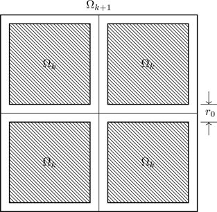
exists and is a function only of n and T. Equation (4.88) follows from the usual thermodynamic formulas (such as in Eq. (4.58)) if Eq. (4.89) holds. We proceed by analyzing a macroscopic system as a sequence of nested domains Ωk, k=1,2,⋯, with volumes Vk<Vk+1 containing Nk particles such that Nk/Vk is fixed38 (see Fig. 4.1). The partition function for the kth domain is
Figure 4.1Domain Ωk+1 is composed of eight domains Ωk (third dimension not shown). Shading indicates the volume accessible to integration in evaluating the partition function.
The notation ∑i<j indicates to sum over i and j such that i<j, which ensures that interactions between particles i and j are counted only once. Equation (4.90) should be compared with Eq. (4.47) where the thermal wavelength λT occurs as a result of integrating the momentum variables. Integration over spatial coordinates is trivial in Eq. (4.47) because it pertains to free particles. The difficult step in evaluating partition functions is always taking into account inter-particle interactions. In what follows, we’ll use a quantity ψk related to the free energy per particle,
ψk≡1NklnZk=−β(FNk/Nk).
(4.91)
For which potentials ϕ(r) and which domains Ωk does limk→∞ψk=ψ(n,T) exist? We won’t dwell on the issue of domains—almost any shape will work (we’ll use cubes), as long as the surface area doesn’t increase too rapidly (more than V2/3 is too fast). The function ϕ(r) must have a repulsive component at short distances together with a long-range attractive component.39 For simplicity, we assume that ϕ has a hard core, ϕ(r)=∞ for r≤r0, and ϕ(r)=0 for r≥b:
ϕ(r)=∞r≤r0<0r0<r<b0r≥b.
(4.92)
Potentials having the form of Eq. (4.92) are known as Van Hove potentials.40
The domain Ωk+1 is composed of eight identical cubes Ωk, each containing Nk particles; thus Nk+1=8Nk and Vk+1=8Vk. Figure 4.1 doesn’t show the third dimension; there are four more cubes not shown. The partition function for domain k+1 is
Imagine letting the cubes in Fig. 4.1 move away from each other far enough that the inter-cube distance exceeds the length b in ϕ(r). In that case the cubes are noninteracting, and
Zk+1noninteracting(Nk+1,Ωk+1,T)=Zk(Nk,Ωk,T)8.
Now restore the cubes to their positions. In doing so, attractive interactions develop between them ( ϕ(r)<0 for r0<r<b). The sum in Eq. (4.93), ∑i<jϕ(|ri−rj|), is therefore more negative than it would be for noninteracting cubes, implying the inequality
Zk+1(8Nk,Ωk+1,T)>Zk(Nk,Ωk,T)8.
(4.94)
Inequality (4.94), combined with Eq. (4.91), implies ψk+1>ψk, a key part of the proof. The sequence {ψk}k=1∞ is an increasing sequence which has a limit if it’s bounded above.41 The sequence will be naturally bounded if, for all configurations of the coordinates r1,…,rN,
∑1≤i<j≤Nϕ(|ri−rj|)>−NB,
(4.95)
where B>0 is independent of N, i.e., if there is a minimum potential-energy configuration of the system (a reasonable request). Making use of inequality (4.95), we have an inequality on Z:
Because V/N is fixed (thermodynamic limit), the right side of (4.97) supplies an upper bound on ψ (see Exercise 4.33), which exists in the desired form, limk→∞ψk=ψ(n,T).
The thermodynamic limit therefore exists, which we can write in the form of Eq. (4.89),
Our proof, however, is based on unphysical assumptions—hard-core potential at short distances and an attractive tail that vanishes at finite distance. It can be made rigorous.[42] Sufficient conditions on ϕ(r) for the thermodynamic limit to exist are that: 1) ϕ(r)≥−a; 2) |ϕ(r)|≤C/rd+ϵ as r→∞, where d is the physical dimension of the system; and 3) ϕ(r)≥C′/rd+ϵ′ as r→0. As mentioned on page 3, the thermodynamic limit exists for systems featuring pure Coulomb forces (no hard core).[37] One must invoke quantum mechanics for such systems, otherwise inequality (4.95) will not hold.42 At least one of the species of particles in the system must obey Fermi statistics, so that the Pauli exclusion principle provides the role of a hard core (see Section 5.5.3).
Stability of the equilibrium state was treated in Sections 1.12 and 2.4 from the perspective of thermodynamics, that for entropy changes associated with fluctuations, d2S<0, which implies that CV>0,βT>0. We now show that CV>0,βT>0 follow readily from the convexity properties of the free energy function, which can be established using the methods of statistical mechanics.
From Eq. (P1.5),
CV=−T∂2F∂T2V.
(4.99)
Invoking CV>0 implies F is a concave function of T, (∂2F/∂T2)V<0. If the convexity properties of F(N,V,T) were independently known, we could use Eq. (4.99) to conclude immediately that CV>0. The partition function is log-convex, ∂2lnZ/∂β2>0 (Eq. (4.17)), implying F is a concave function of T; see Exercise 4.24. By the very structure of statistical mechanics (that the partition function is the Laplace transform of the density of states function, Section 4.1.4), we know once and for all that F is a concave function of T.
It’s a little more involved to show that F(N,V,T)is a convex function of N and V, which has as a consequence that βT>0. Referring to Fig. 4.1, where the domain Ωk+1 is constructed from eight cubes Ωk, consider that we place Nk(1) particles into each of four Ωk cubes, and Nk(2) particles into the remaining four, so that Nk+1=4(Nk(1)+Nk(2)). Keeping n1≡Nk(1)/Vk and n2≡Nk(2)/Vk fixed, we have, using the reasoning leading to (4.94), the inequality,
Define (instead of Eq. (4.91)) a quantity related to the free energy per volume,
gk(ni)≡Vk−1lnZ(Nk(i),Ωk,T)=−βFNk/Vk.(i=1,2)
(4.101)
From Eq. (4.91), gk=(Nk/Vk)ψk. Because limk→∞ψk exists (see Section 4.2), limk→∞gk exists, and we can write (compare with Eq. (4.98))
limV→∞FV=−kTg(n,T).
We now show that g(n,T) is a concave function of n, implying that the free energy per volume is a convex function of n.
Using inequality (4.100) and Eq. (4.101), we infer the inequality
gk+1(12(nk(1)+nk(2)))>12gk(nk(1))+g(nk(2)),
where we’ve used Vk+1=8Vk. In the limit k→∞ (the sequence {gk} is monotonically increasing), we have
g(12(n1+n2))>12g(n1)+g(n2).
(4.102)
Thus, g(n) is a concave function (see Fig. 4.2), that the value of the function at the midpoint of an arc is not less than the mean of the values of the function at the two end points of the arc. The defining property (4.102) generalizes (because g(n) is bounded and hence continuous43) to[45]
Figure 4.2Concave function g(n). The chord joining any two points on the graph of the function lies below the graph. More generally, for concave functions g(ωn)≥ωg(n) for 0≤ω≤1.
g(ωn)≥ωg(n)(0≤ω≤1)
(4.103)
if we agree to the reasonable request that g(0)=0, which follows by demanding that the partition function of zero particles is unity, Z(0,V,T)=1. The derivative dg/dn of a continuous concave function g(n) is such that, an any point, the right derivative is not greater than the left derivative, with both derivatives non-increasing functions of n.
By definition, g(n)=v−1ψ(v), where v≡V/N=n−1. Using (4.103), we have
ψ(v)≤ψ(v′),whenv≤v′
(4.104)
i.e., ψ(v) is a monotonic, nondecreasing function of v. Using Eq. (1.14) and F=−NkTψ,
P=−∂F∂VT,N=kTN∂ψ∂VT,N=kT∂ψ∂vT,N.
Using the properties of the derivative of concave functions stated above, we conclude that pressure is a monotonic nonincreasing function of the specific volume, ∂P/∂vT,N<0 —the larger the volume per particle, the lower the pressure (at a fixed temperature). And, because P(v) is monotonic, its derivative exists, and thus so does its inverse, the isothermal compressibility:
βT≡−1V∂V∂PT,N=−1V1∂P/∂VT,N=−1v1∂P/∂vT,N>0.
(4.105)
Thus, βT>0 occurs naturally in the formalism of statistical mechanics. From Exercises 4.35 and 4.36, we can use βT>0 to establish the convexity properties of F(N,V,T) and G(N,P,T). To summarize:
Statistical mechanics requires modification when the quantum nature of matter is taken into account. The derivation of the canonical distribution in Section 4.1.7 invoked energy equipartition, Eq. (4.37), that the kinetic energy per particle E/N=32kT, implying that the specific heat is independent of T. The validity of that assumption breaks down at low temperature—specific heats vanish as T→0; we have to start over in devising a quantum statistical mechanics.
Consider a gas of diatomic molecules (which we treat in Section 5.4), such as HCl. The Hamiltonian for a rigid diatomic molecule consisting of structureless atoms has five additive quadratic degrees of freedom: three for the motion of the center of mass and two associated with angular momentum about the center of mass.44 Assuming energy equipartition, we expect the specific heat to be 52k, and this is what is observed (at room temperature). Shouldn’t we expect, however, that the atoms vibrate with respect to each other? In that case there would be two additional quadratic degrees of freedom in the Hamiltonian (the kinetic and potential energies of vibration), implying that the specific heat should be 72k. Experiment shows that as the temperature is raised (but before the molecule dissociates), the value of the specific heat rises towards 72k. At room temperature, therefore, molecular vibrational degrees of freedom are ineffective—they don’t become excited. Moreover, we know that atoms are not structureless and have internal, electronic degrees of freedom. Their failure to be represented in the value of the specific heat indicates that atomic degrees of freedom are ineffective. Not all degrees of freedom participate equally in becoming excited so as to be able to absorb energy at a given temperature (in contradistinction to the equipartition theorem). That specific heats vanish as T→0 suggests that all degrees of freedom become ineffective at low temperature, something beyond the ability of classical mechanics to describe.
The breakdown in our energy-equipartition-based formalism occurs when the mean energies it predicts become sufficiently small (be they related to translation, or rotation, or—whatever). It’s here that quantum mechanics must replace classical dynamics, because the motions in question cannot be even approximately described by means of classical dynamics. Under these circumstances, what we have hitherto taken to be microstates is meaningless. We can no longer use phase space to represent microstates. Move over Γ-space, here comes Hilbert space.
The state of a quantum system is denoted by the Zen-like symbol |ψ〉, the state vector. The wavefunction, ψ(x), such that |ψ(x)|2 is a probability density, is the abstract vector |ψ〉 expressed in the position basis: ψ(x)≡〈x|ψ〉, where the angular brackets denote an inner product defined on the Hilbert space of all possible quantum states. The wavefunction is a function of the spatial coordinates of the particles of the system (“half” of phase space). There can also be internal degrees of freedom, so the wavefunction depends on a set of quantum numbers. For electrons, the wavefunction is written ψσ1,⋯,σN(r1,⋯,rN), where σi=±12. In order not to burden the notation, we won’t write these indices.
Observable, i.e., measurable quantities, which in classical mechanics are phase-space functions A(p,q), are in quantum mechanics represented as Hermitian operators, A^. We noted in Section 2.4 that fluctuations force us to interpret the measured values of macroscopic quantities as the mean of a large number of measurements. In quantum mechanics we have another source of indeterminacy: Measurements made on a system prepared in a known state occur with a range of values, and thus even for a well defined quantum system we must seek the mean of a number of measurements. Whereas in classical mechanics the trajectory of a particle subject to the same forces given the same initial conditions is reproducibly the same, in quantum mechanics measurements made on identically prepared systems do not produce the same values—the extra “layer” of indeterminism noted in Section 2.7. The expectation valueA¯ψ of a large number of measurements of A^ on systems prepared in state |ψ〉 is found from
A¯ψ=∫dxψ*(x)A^ψ(x)≡〈ψ|A^ψ〉,
(4.106)
when |ψ〉 is normalized, 〈ψ|ψ〉=1. The act of measurement introduces an uncontrollable interaction with the system that modifies what we seek to measure. To see this, make use of the eigenfunctions of A^, a set of functions {ϕn(x)}n=0∞ such that A^ϕn=λnϕn, where (because A^ is Hermitian) the eigenvalues λn are real numbers and the eigenfunctions are orthonormal, 〈ϕn|ϕm〉=δnm. Eigenfunctions of Hermitian operators are also complete sets, whereby an arbitrary square-integrable function ψ(x) can be represented by an infinite linear combination,45
ψ(x)=∑n=0∞anϕn(x),
(4.107)
where the expansion coefficients (probability amplitudes) an=〈ϕn|ψ〉. Because |ψ〉 is normalized,
∑n=0∞|an|2=1.
(4.108)
Combining Eqs. (4.106) and (4.107),
〈ψ|A^ψ〉=∑n=0∞|an|2λn.
(4.109)
Thus, the expectation value of A^ on systems in state |ψ〉 is an average of the eigenvalues of A^, which occur with a probability distribution |an|2=|〈ϕn|ψ〉|2 (see Eq. (4.108)), and, as such, is an averaging process related to the probabilistic aspect of wavefunctions. To what extent can the quantum states of a system be controlled? As we now show, we must introduce a second kind of average over the quantum states of a system—the ensemble average.
Statistical mechanics employs wavefunctions of many particle systems, which often entail identical particles, and here we run into a new piece of physics, the indistinguishability of identical particles. Wavefunctions of an assembly of identical particles are either symmetric or antisymmetric under a permutation of any two particles (see Appendix D). Under the interchange of particles at positions rj and rk (leaving all other particles unchanged), the basic principles of quantum mechanics require that (for identical particles)
ψ(⋯,rj,⋯,rk,⋯)=θψ(⋯,rk,⋯,rj,⋯),
(4.110)
where
θ={+1forbosons−1forfermions
In either case, the probability density is invariant under the interchange of particles, ψ(⋯,rk,⋯,rl,⋯)2=ψ(⋯,rl,⋯,rk,⋯)2, implying that identical particles can’t be labeled.46 To construct an N-particle wavefunction, we use as basis functions, products of N single-particle wavefunctions,47
where the functions {ϕk} are a complete set (which could be plane-wave functions or atomic wave functions—whatever is most convenient for the problem at hand), and where c(m1,⋯,mN) are expansion coefficients. Equation (4.111) is to many particle wavefunctions what Eq. (4.107) is to single particle wavefunctions. The expansion coefficients c(m1,⋯,mN) “do the work” of providing the proper exchange symmetries (because the basis functions do not), i.e.,
c(⋯,mk,⋯,ml,⋯)=θc(⋯,ml,⋯,mk,⋯).
Note that if ml=mk=m, antisymmetry requires that c(⋯,m,⋯,m,⋯)=0, the usual form of the Pauli principle for fermions.
To avoid cumbersome notation, let’s express Eq. (4.111) as
ψ(x)=∑rcrϕr(x),
(4.112)
so that r is a multi-index symbol. The expectation value of A^ is then (see Exercise 4.37; we’re not using a basis of eigenfunctions),
A¯=〈ψ|A^ψ〉=∑r∑scr*cs〈r|A^s〉≡∑r∑scr*csArs,
(4.113)
where Ars=〈r|A^s〉 are the matrix elements of A^, in the basis set used in Eq. (4.111).48
A system known to be in state |ψ〉 is said to be in a pure state. It’s almost always the case that we have incomplete knowledge of the microscopic state of the system. And what do we do in the face of incomplete knowledge? I hope you’re saying: “Resort to probability.” Let γi denote the probability that a randomly selected member of the ensemble is in state |ψ(i)〉, such that
∑iγi=1.
(4.114)
The wavefunction ψ(i)(x) of each possible state49 can be expressed as in Eq. (4.112):
ψ(i)(x)=∑rcr(i)ϕr(x).
The expectation value of A^ in state |ψ(i)〉 is, from Eq. (4.113),
A¯(i)=∑r∑scr(i)*cs(i)Ars.
The ensemble average of a measurable quantity A^ is defined as
A≡∑iγiA¯(i)=∑iγi∑r∑scr(i)*cs(i)Ars.
(4.115)
There are two averaging processes here: the quantum expectation value A¯(i) of A^ in state |ψ(i)〉, together with a thermal average over the states |ψ(i)〉, which occur with probabilities γi.
Based on Eq. (4.115), define a matrix, the density matrixρ (which represents the ensemble), with elements (note the order of the indices)
ρsr≡∑iγics(i)cr(i)*.
(4.116)
Combining Eq. (4.116) with Eq. (4.115),
A=∑r∑sρsrArs=∑sρAss=TrρA,
where we’ve used the rules of matrix multiplication, and where the trace of a matrix is the sum of its diagonal elements: TrM≡∑sMss. Prior experience with quantum mechanics indicates that we should seek an operator to take the place of the phase-space probability functions of classical statistical mechanics. We define the density operator (or statistical operator) ρ^, which has for matrix elements those of the density matrix ρsr,
ρsr≡∫ϕs*(x)ρ^ϕr(x)dx=〈s|ρ^r〉.
The ensemble average can then be written
A=∑s∑rρsrArs=Tr(ρA)=Trρ^A^=TrA^ρ^.
(4.117)
Now, the trace is independent of the basis in which the matrix elements of an operator are defined.[16] Thus, we can associate the trace with the operator itself—hence the right side of Eq. (4.117). We’ve also used the cyclic invariance of the trace, TrAB=TrBA; see Exercise 4.38. Note that
where we’ve used Eq. (4.108), true for normalized wavefunctions, and Eq. (4.114).
You may wish to refer to Section 2.5.1 to see how ensemble averages were defined for classical systems; Eqs. (4.117) and (4.118) are the quantum analogs of Eqs. (2.53) and (2.52). We’ve replaced the phase-space averages of classical statistical mechanics, 〈A〉=∫ΓA(p,q)ρ(p,q)dΓ, involving probability density functionsρ(p,q), with the trace of the density operator ρ^ acting on the operator A^ representing the observable, 〈A〉=Trρ^A^.
New features appear in quantum statistical mechanics that have no classical counterpart. Write Eq. (4.117), separating the diagonal from the off-diagonal matrix elements,
A=∑sρssAss+∑s∑r≠sρsrArs.
(4.119)
From Eq. (4.116), ρss=∑iγi|cs(i)|2≥0, and from Eq. (4.118), ∑sρss=1: Thus, the diagonal element ρss is the probability of finding the system in state s. The off-diagonal elements, however, have no definite sign and cannot be interpreted as probabilities.50 These terms arise from the wave nature of matter and are without classical counterpart; they’re linked to the interference effects observed in experiments such as electron diffraction. If in a given basis the density matrix is diagonal ( ρrs=0 for r≠s), the definition of 〈A〉 in Eq. (4.119) is the same as in the classical theory when restricted to discrete probabilities. While the density matrix might be diagonal in a special basis, the diagonal character of a matrix is not basis-independent.
The density operator can be treated in a way that’s independent of the basis used to define its matrix elements. It can be shown[17, Chapter 5] that ρ^(t), generalized to include time,51 satisfies a differential equation, the von Neumann equation,
iℏ∂∂tρ^(t)=H^,ρ^(t),
(4.120)
where [H^,ρ^] denotes the commutator, [A,B]≡AB−BA. The von Neumann equation is the analog of the Liouville equation, Eq. (2.55); it’s the fundamental equation of quantum statistical mechanics. Quantum statistical mechanics may be said to be the study of the solutions of Eq. (4.120).
Ensembles of equilibrium systems are stationary, ∂ρ^/∂t=0, implying that ρ^ commutes with the Hamiltonian,52[H^,ρ^]=0. Commuting operators have a common set of eigenfunctions.53 Using the eigenfunctions of H^ as a basis (the energy representation), the density matrix is diagonal (see Exercise 4.40),
ρrs=ρrδrs.
(4.121)
In what follows, we work with the density matrix in the energy representation.
4.4.1 Microcanonical ensemble
Consider an ensemble of isolated systems having a fixed number of particles in a fixed volume. The density matrix is diagonal, as in Eq. (4.121), with
ρr=1ΩifE=Er0otherwise,
where Ω is the number of states available to the system at energy Er.
4.4.2 Canonical ensemble
Consider an ensemble of systems with well defined values of N, V, T. The probability that a randomly chosen system has energy En is proportional to the Boltzmann factor. The density matrix is diagonal as in Eq. (4.121) with
ρn=1Z(β)gne−βEn,
(4.122)
where Z(β) is defined in terms of the discrete energies
Z(β)=∑ngne−βEn,
(4.123)
where gn is the degeneracy of the nth energy level, the number of linearly independent eigenfunctions each having eigenvalue En. The density operator in the canonical ensemble may be evaluated using Eq. (P4.14),
where we’ve used that e−βH^ϕn=e−βEnϕn, Eq. (P4.16), and the completeness relation, Eq. (P4.15). The ensemble average of an observable quantity A is therefore
〈A〉=Trρ^A^=1ZTre−βH^A^=1Z(β)∑ngne−βEn〈ϕn|A^ϕn〉.
(4.125)
4.4.3 Grand canonical ensemble
The density operator in this case must commute with the Hamiltonian and the number operatorN^ whose eigenvalues are 0,1,2,… (see Appendix D). The density operator is
ρ^=1ZGe−β(H^−μN^),
(4.126)
where
ZG=Tre−β(H^−μN^)=∑N=0∞eβμNZN(β)
(4.127)
is the grand partition function, with ZN the canonical partition function for an N-particle system. Ensemble averages are then given by
〈A〉=1ZG∑N=0∞eβμNZN(β)〈A〉N,
(4.128)
where 〈A〉N denotes the canonical ensemble average for an N-particle system.
Summary
In this chapter, we developed the ensemble formalism of statistical mechanics (a huge undertaking, by the way; Chapter Statistical Mechanics is foundational and is no doubt the most difficult in this book). In doing so, it concludes the first part of this book, Chapters 1–Statistical Mechanics. The aforementioned quote by R.P. Feynman aptly pertains to the organization of this book: Part I covers theoretical foundations, culminating in the derivation of the Boltzmann distribution, with Part II devoted to applications.
The phase-space probability density for isolated classical systems (fixed N,V,E) is
ρ(p,q)=1Ω(E)δ(E−H(p,q)),
where Ω(E) is the density of states function for the system (which depends on the external variables V and N). The density of states function plays a fundamental role in the theory. There is a tendency in teaching statistical mechanics to impart the impression that the density of states function is a convenient quantity that allows us to convert integrations over Γ-space (or k-space) to integrations over the energy. While true, we’ve seen that Ω(E) makes an early entrance into the foundations of the subject. The density of states function isn’t simply convenient, it’s essential. Expressions for the density of states of free, nonrelativistic particles and photons were derived in Section 2.1.5. The density of states of free, relativistic, massive particles is developed in Section 5.7.1.
The phase-space probability density for closed classical systems (fixed N,V,T) is
ρ(p,q)=1N!Zcane−βH(p,q)⇒ρ(E)=1N!Zcane−βEΩ(E),
where β=1/(kT) and the normalizing factor, the partition function, is given by
Zcan(N,V,T)=1N!∫e−βH(p,q)dΓ=1N!∫e−βEΩ(E)dE,
where the Hamiltonian is a function of the external parameters V and N. The presence of N! is required to prevent overcounting configurations of identical particles (which are invariant under permutations of the particles). Except for calculations of entropy ( S=−kβ2∂β−1lnZcan/∂β, Eq. (4.56)), the factor of N! is unnecessary in calculations involving logarithmic derivatives of the partition function, such as for the average internal energy.
The partition function is the Laplace transform of the density of states function,
Z(β)=∫0∞e−βEΩ(E)dE,
which shows why it serves as the normalization factor on the probability density. The Boltzmann factor e−βE is the extent to which the energy states of the system are populated at temperature T, and Ω(E)dE is the number of energy states between E and E+dE. Thus Z=∫0∞e−βEΩ(E)dE is the total number of possible states accessible to the system at temperature T. The probability P(E)dE=e−βEΩ(E)dE/Z is the ratio of two numbers: the number of states available to the system at energy E when it has temperature T, to the total number of states available to the system at temperature T.
For open classical systems (fixed μ,V,T), we can’t write down a simple formula for the phase-space probability density, because ensemble averages involve integrations over phase spaces of varying dimensionality. The ensemble average of a phase-space function A(p,q,N) (that depends on the number of particles) is, by combining Eqs. (4.73) and (4.75),
Ensembles are specified by given thermodynamic variables, whereas other thermodynamic quantities are obtained from derivatives of Z. In the canonical ensemble there is a connection between Z and the Helmholtz energy F(N,V,T), from Eq. (4.57),
Zcan=e−βF.
In the grand canonical ensemble the partition function is related to the grand potential Φ(μ,V,T), from Eq. (4.76),
ZG=e−βΦ.
The thermodynamic variables associated with the ensembles are summarized in Table 4.1. Each ensemble involves seven thermodynamic variables, those connected by the Euler relation, Eq. (1.53). The normalizing factor in the microcanonical ensemble, Ω(E), is related to the entropy through the Boltzmann relation, Ω=exp(S/k).
Table 4.1 Statistical ensembles and their associated thermodynamic variables
Ensemble
Fundamental variables
Thermodynamic potential
Implied variables
Microcanonical
U,V,N
S(U,V,N)
T,P,μ
Canonical
T,V,N
F(T,V,N)
S,P,μ,U
Grand canonical
T,V,μ
Φ(T,V,μ)
S,P,N,U
From first derivatives of Z one can calculate various ensemble averages. In the canonical ensemble (variable energy), the average energy is, from Eq. (4.40),
U=〈H〉=−∂∂βlnZcanV.
The values of (μ,P,S) can be calculated using Eq. (4.58) and knowledge of the Hamiltonian. In the grand canonical ensemble (varying energy and particle number), the average number of particles is, from Eq. (4.78),
〈N〉=∂∂(βμ)lnZGT,V.
One can calculate P and S using the other expressions in Eq. (4.78). The average energy is obtained from Eq. (4.82),
U=〈H〉=−∂lnZG∂βz,V,
where z≡eβμ is the fugacity. In the canonical ensemble, the chemical potential μ=μ(N,V,T) is a function of particle number (from Eq. (4.45)), whereas in the grand canonical ensemble N=N(μ,V,T) is a function of the chemical potential (from Eq. (4.78)).
From second derivatives of Z, one can calculate the values of fluctuations. In the canonical ensemble, from Eqs. (4.61) and (4.62), we have that the heat capacity is a measure of energy fluctuations:
∂2lnZcan∂β2=H2−〈H〉2=H−〈H〉2=kT2CV.
In the grand canonical ensemble, we have that the isothermal compressibility βT is a measure of fluctuations in particle number. From Eq. (4.81),
N2−〈N〉2=∂2lnZG∂(βμ)2=kTN2VβT.
Energy fluctuations in the grand canonical ensemble are, from Eq. (4.87),
H2−〈H〉2=kT2CV+(N−〈N〉)2∂U∂NT,V2.
The relative root-mean-square deviations
H−〈H〉2〈H〉N−〈N〉2〈N〉
are of order N−1/2≈10−12 for Avogadro’s number.
Thermodynamic relations derived in the different ensembles are not in general the same for finite-size systems. They become identical for macroscopic systems which we can model with the limit N→∞. The limiting process N→∞, V→∞, but with N/V fixed, is known as the thermodynamic limit. We presented an outline of the proof of the existence of the thermodynamic limit. A nodding acquaintance with the thermodynamic limit will be required in the subsequent developments in this book.
The thermodynamic theory of the stability of the equilibrium state (discussed in Sections 1.12 and 2.4) shows that CV>0 and βT>0 from an analysis of entropy changes produced by fluctuations. The same conclusions follow in statistical mechanics from the convexity properties of the Helmholtz energy, F(N,V,T); see Section 4.3.
In quantum statistical mechanics (Section 4.4), we transition from phase space descriptions to a picture that focuses on the energy levels of systems, or, more generally, on the eigenvalues of Hermitian operators that represent physical observables. We also transition away from probability density functions (in classical statistical mechanics) to a probability density operator, ρ^, with ensemble averages of an observable A given by Eq. (4.117), A=Trρ^A^, where, to make use of the trace operation, we must declare a basis in which to evaluate the matrix elements of the operators ρ^ and A^. Fortunately, the trace is independent of basis. In a basis of the eigenstates of the Hamiltonian, the density matrix is diagonal. In that case, averages in the canonical and grand canonical ensemble are given by Eqs. (4.125) and (4.128).
Having now developed the basic formalism of statistical mechanics, it’s instructive to return to the beginning of this chapter and consider where it comes from. Equation (4.1) is entirely from the theory of probability, with little input from physics, other than the Hamiltonian defines a constant-energy hypersurface in Γ-space, H(p,q)=E. The Hamiltonian is in fact all the physics it can have. The equilibrium probability distribution is stationary, ∂ρ/∂t=0, implying from Liouville’s theorem that ρ is a function of H. The Hamiltonian is the “place” where microscopic information about the components of the system enters the theory. Most results in the theory of probability are based on the assumption of equal probabilities of elementary events, implying that if we draw on the methods of probability, we’ve signed off on that assumption. Lacking precise information to the contrary, we have no basis on which not to assume that microscopic events occur with equal likelihood. Ensembles are our answer to the problem that we as humans lack the ability to control the microscopic events underlying macroscopic systems; ensembles are abstract collections of identical copies of a system that embody all possible initial conditions consistent with known macroscopic information. Some books take the microcanonical distribution function, Eq. (4.3), as a postulate because it effectively embodies the ergodic hypothesis (phase trajectories uniformly cover a constant-energy surface). We argued in Chapter 2 that the ergodic hypothesis is not necessary for the construction of statistical mechanics—we’re free to adopt whatever assumptions we require so long as they’re sufficient to guarantee that the laws of thermodynamics emerge from the statistical theory. There are books that take the canonical distribution function as a postulate as well, Eq. (4.32). The derivation of Eq. (4.13) relied on the geometry of Γ-space and requires only that the density of states function exists; it has almost no physics in it other than the assumption of weakly interacting subsystems (energy of interaction between subsystems negligible in relation to bulk energies, a picture justified by the existence of the thermodynamic limit). The subsequent derivation from Eq. (4.13) to Eq. (4.32) invoked the central limit theorem which relies on the large number of components systems have; therein lies the universality of statistical mechanics—it applies to any macroscopic system. As an alternative (acknowledging that a fundamental law of nature—the Boltzmann distribution—cannot be derived from something more fundamental), we derived the canonical distribution starting from the microcanonical distribution of an isolated compound system by eliminating the environmental degrees of freedom (in reducing a joint probability density of the compound system to the probability density of a single system that interacts with its environment). In that approach we encountered the assumption of energy equipartition, implying the temperature-independence of the heat capacity—true of many materials—but which ultimately can’t be justified at low temperature, signaling the need for a theory based on quantum mechanics. Statistical mechanics inherits quite a bit of structure from the theory of thermodynamics (which underscores why it’s really helpful to understand thermodynamics in its own right). Once it’s been shown that statistical mechanics is consistent with the second law of thermodynamics, Eq. (4.45), we’re free to make use of relations derived in thermodynamics, knowing that points of contact occur between the partition function and the relevant thermodynamic potential associated with the types of systems comprising the ensemble. Out of this melange of ideas, can we pinpoint the essential ideas that the edifice of statistical mechanics rests on—equal a priori probabilities, weakly interacting systems, energy equipartition? The thermodynamic limit, on which extensivity is based, requires a system to possess a minimum-potential-energy-configuration. Perhaps the essential idea is simply randomness—that which is not under our control we can only assume occurs randomly. And at that point, the theory of probability takes over.
EXERCISES
4.1Derive Eq. (2.19).
4.2Consider a system of free particles confined to two dimensions. There are several ways, for example, to confine electrons in semiconductor devices to two-dimensional regions (because motion in the third dimension is precluded by a confining potential). Repeat the calculations from Eqs. (2.15) to (2.17) for particles confined to an area A to derive an expression for the density of single-particle states. A: gdAm/(2πℏ2). Hint: What is the size of the unit cell for a two-dimensional k-space?
4.3Derive the density of states of a free relativistic particle of rest mass m in three spatial dimensions of volume V. Show that
g(T)=gdV2π2(ℏc)3T2+2Tmc2(T+mc2),
where T indicates the kinetic energy of the particle, with E=(pc)2+(mc2)2=T+mc2. If this seems like a difficult problem (and it kind of is a difficult problem), look ahead to Section 5.7.
Hint: Use the beta function defined in Appendix B.
4.5Show that the nth moment of Ω(x) can be found by taking derivatives of the partition function,
〈xn〉=1Z(α)(−1)ndndαnZ(α).
The partition function can then be referred to as the generating function for the density of states function; see Section 3.5.3.
4.6Derive Eq. (4.16) starting from Eq. (4.9). Keep in mind that Ω(x)=0 for x≤0.
4.7Derive Eq. (4.17).
4.8Derive Eqs. (4.20) and (4.21) using Eq. (4.19).
4.9Derive the results in Eq. (4.24) by substituting Eq. (4.23) into Eqs. (4.20) and (4.21).
4.10Consider the function f(x)=eαxe−βx2 ( α,β>0), the product of an exponential function and a Gaussian function centered about the origin. Find the location x=x* where f(x) has a maximum (A: x*=α/2β). Show that f(x) is a Gaussian centered about a new mean:
f(x)=eα2/4βe−β(x−x*)2.
Hint: Complete the square. Thus, multiplying a Gaussian by an exponential function results in another Gaussian that’s centered about a new location and that’s been scaled in magnitude, but which retains the width of the original Gaussian, ≈1/β.
4.11Derive Eq. (4.35). Hint: Use Eq. (B.14) and the properties of the gamma function.
4.12Work through the steps in Eq. (4.36).
4.13What’s the Hamiltonian for a system of N structureless particles of mass m contained in a rigid container of volume V? Hint: This is a trick question. Ordinarily one would say that H is the kinetic energy, H=(1/(2m))∑i=13Npi2. To take into account the finite volume, one should add to H a function, call it θ(q), such that θ(q)=0 or ∞ depending on whether the values of qk correspond to points inside or outside the container; θ(q) is formally the potential associated with an external force that confines the particles to a finite volume.
4.14Show that
CV=kβ2∂2∂β2lnZV.
(P4.1)
4.15Derive Eqs. (4.41) and (4.42).
4.16Show the identities (which hold for any smooth function Z, i.e., these identities are obtained using calculus)
β∂∂ββ−1lnZ=∂lnZ∂β−1βlnZ.
∂∂ββ2∂∂ββ−1lnZ=β∂2lnZ∂β2.
4.17Fill in the steps leading to Eq. (4.45).
4.18For the canonical ensemble with ρ=e−βH/Z and Z=∫e−βHdΓ:
Show that variations in ρ, δρ, are given by (for the variation symbol δ defined in Eq. (4.44)),
where δm refers to mechanical variations in external parameters, δmH≡∑i∂H/∂XiδXi.
Show that ∫δρdΓ=0, i.e., variations of the normalization condition ∫ρdΓ=1 vanish.
Equation (4.43) defines the heat transferred to a system as the difference between variations in internal energy (produced by any means) and adiabatic work. Show that
δQ=∫HδρdΓ=−(H2−H2)δβ−β(HδmH−〈H〉δmH).
Note that δQ is not an ensemble average in the usual sense.
4.19Derive Eq. (4.46) from Eq. (4.45), taking into account that the thermodynamic definition of entropy is (đQ)rev/T=dS. Hint: ∂/∂β=(∂T/∂β)∂/∂T=(−1/(kβ2))∂/∂T.
4.20Verify Eq. (4.47) for an ideal gas contained in volume V in equilibrium with its environment at absolute temperature T.
4.21Is Eq. (4.55) satisfied by partition function of the ideal gas?
4.22Consider a gas of relativistic particles, for which the density of states for a single relativistic particle was derived in Exercise 4.4. What is the equation of state of such a system? A: PV=NkT. Hint: The partition function for N free particles is Z=(Z1)N, where Z1 is the partition function of a single particle. Show that Z1 has the form Z1=Vf(T), where T is the temperature. Using Eq. (4.58), you don’t have to know the explicit form of f(T).
4.23Verify all parts of Eq. (4.61).
4.24Show in the canonical ensemble that, as an exercise in the chain rule,
∂2lnZ∂β2=−kT3∂2F∂T2.
Argue therefore that
∂2F∂T2<0,
and hence that F(N,V,T) is a concave function of T. Hint: H−〈H〉2≥0 from Eq. (4.61), or see Eq. (4.17).
4.25Consider a system that interacts with an external magnetic field, H. Which ensemble should we use to predict its thermodynamic behavior? What are the relevant variables for such systems? Start with the first law of thermodynamics. The work done on a system in reversibly changing its magnetization by dM is dW=μ0HdM=BdM. The first law for such a system is
dU=TdS−PdV+μ0HdM+μdN.
Assume in experiments on such systems that PdV work is negligible. The first law simplifies: dU=TdS+BdM+μdN. Thus, U=U(S,M,N). Define the magnetic Gibbs energy,
Gm≡U−TS−BM=F−BM.
(P4.2)
Form its differential,
dGm=−SdT−MdB+μdN,
(P4.3)
and therefore Gm=Gm(T,B,N). Work in the T,B,N ensemble.
Show that Eq. (P4.3) implies the thermodynamic identities,
S=−∂Gm∂TB,NM=−∂Gm∂BT,Nμ=∂Gm∂NT,B,
(P4.4)
and the Maxwell relation
∂M∂TB,N=∂S∂BT,N.
(P4.5)
The magnetization M is the sum of the individual magnetic dipole moments of the particles of the system, M≡∑i=1Nmi, with the energy of interaction with the field given by E[m1,m2,⋯,mN]=−B∑i=1Nmi. (The notation E[m1,m2,⋯,mN] indicates that E depends on the configuration of all the magnetic moments.) The partition function is then given by (we’re ignoring translational kinetic energy of the dipoles—they could be located on the sites of a crystalline lattice):
where ∑{mi} indicates a sum over all configurations of the dipoles. (We’re being a bit obscure here; we get more precise in Section 5.2.) Show that
Gm(T,B,N)=−kTlnZ(T,B,N)−BM(T,B,N),
where
M(T,B,N)=∂∂(βB)lnZ(T,B,N).
Hint: Use Eqs. (4.40) and (4.46), and make use of ∂/∂T=−(β/T)∂/∂β. Thus we have
Z(T,B,N)=exp−β[Gm(T,B,N)+BM(T,B,N)]≡e−βF(T,B,N),
where Gm+BM effectively defines a Helmholtz energy as a function of (T,B,N).
Referring to the magnetic susceptibility χ≡∂M/∂BT, Eq. (1.50), show that
χ=β〈M2〉−〈M〉2=β〈M−〈M〉2〉.
(P4.6)
The susceptibility is thus a measure of fluctuations in the magnetization, just as CV is a measure of energy fluctuations, Eq. (4.62), and the compressibility βT is a measure of particle fluctuations, Eq. (4.81).
4.26Derive Eq. (4.70). Start with Eq. (4.67) and re-express it as a relation for dS. Note that S=S(U,Xi,Nj), that S is naturally a function of the extensive variables (U,Xi,Nj). Invoke extensivity, S(λU,λXi,λNj)=λS(U,Xi,Nj), and reach for Euler’s theorem.
4.27Show, by combining Eqs. (4.71) and (4.69), that we have the most general form of the Gibbs-Duhem equation:
∑jNjdμj=−SdT−∑iXidYi.
(P4.7)
Compare with Eq. (P1.1) for a single-component system with V the only external parameter.
4.28From Eq. (4.76), ZG=e−βΦ, and for a single component system with V the only relevant external parameter, Φ=−PV. Thus, in this case, ZG=eβPV. For the ideal gas, therefore, ZG=e〈N〉. Show this is consistent with the expression derived in Eq. (4.79). In the grand canonical ensemble, N is not a known quantity, but rather N=N(μ,T,V).
4.29Derive Eq. (4.77). Show that for Eq. (4.75) to satisfy Eq. (4.74), Eq. (4.77) ensues.
4.30
Show that
∂∂βlnZG|μ=μ〈N〉−U,
where U≡∑N=0∞∫ΓNHNρNdΓN.
Show, for a single-component system having only one relevant external parameter V, that lnZG=V∂lnZG/∂V, implying that lnZG varies linearly with V.
Show for the ideal gas that
∂∂βlnZG|μ=〈N〉μ−32kT.
Use Eq. (4.79). The internal energy of the ideal gas in the grand canonical ensemble is therefore given by the expression U=32〈N〉kT.
Show that the second and third relations in Eq. (4.78) lead to the known expressions for the equation of state and entropy of the ideal gas.
4.31
Show, for ZG=ZG(μ,V,T), that ∂2lnZG∂μ2|T,V=1ZG∂2ZG∂μ2|T,V−∂lnZG∂μ|T,V2. There is no physics in this formula, just calculus.
Show that 1ZG∂2ZG∂μ2|T,V=β2〈N2〉. Hint: Start from Eq. (4.77) and recognize that
〈N2〉=∑N=0∞N2PN=1ZG∑N=0∞N2eβμNZcan(N,V,T).
Using Eq. (4.78), conclude that
〈N2〉−〈N〉2=kT2∂2lnZG∂μ2|T,V=kT∂〈N〉∂μ|T,V.
(P4.8)
4.32Guided exercise to establish the identity in Eq. (4.81),
∂N∂μT,V=N2VβT.
(P4.9)
We do this in steps.
The fundamental variables in the grand canonical ensemble are μ,T,V, from which the average number of particles can be calculated using Eq. (4.78). For simplicity, we use N here to denote 〈N〉. Thus, N=N(μ,T,V), and implicitly, V=V(μ,T,N). We seek to develop an identity for (∂N/∂μ)T,V (look ahead to Eq. (P4.10)). You might want (right now) to consult Table 1.3 and Eq. (P1.8) to see if this derivative occurs in a Maxwell relation. It doesn’t, but it’s always worth a try! From calculus
dN=∂N∂μT,Vdμ+∂N∂Tμ,VdT+∂N∂Vμ,TdV.
We can also expand dV in terms of differentials of μ,T,N. Thus,
These expressions generalize the cyclic relation Eq. (1.31) to four variables, N,μ,T,V.
What do we know about ∂V/∂μT,N ? This derivative is part of a Maxwell relation (see Table 1.3), but I don’t see how it helps us.54 We can get at this derivative through the Gibbs-Duhem equation55 for a single-component system where V is the only relevant external variable, Eq. (P1.1), Ndμ=VdP−SdT. We have in the grand canonical ensemble that N=N(μ,V,T) (implying μ=μ(N,V,T)) and P=P(μ,V,T), implying that P=P(N,V,T). Expand P assuming it’s a function of N,V,T:
Ndμ=V∂P∂NT,VdN+V∂P∂VN,TdV+V∂P∂TN,V−SdT.
Holding T,N fixed,
∂μ∂VT,N=VN∂P∂VN,T=−1NβT.
(P4.11)
Equation (P4.11) is not a Maxwell relation.
Note, however, that Eq. (P4.11) implies
∂μ∂PT,N=VN.
(P4.12)
Using a Maxwell relation, Eq. (P1.8), Eq. (P4.12) implies that
∂N∂Vμ,T=NV.
(P4.13)
Combining Eqs. (P4.10), (P4.11), and (P4.13), we obtain Eq. (P4.9).
4.33Calculate the quantity ψ≡lnZ(N,V,T)/N for the ideal gas. (A: 1+ln(V/NλT3).) Note that the same group of terms appears on the right side of the inequality (4.97).
4.34Show that Eq. (4.104) implies Eq. (4.103). Hint: Let n′=ωn.
4.35Show for the Helmholtz energy F(N,V,T) that
∂2F∂N2T,V=VN2βT. Hint: Use the result derived in Exercise 4.32.
∂2F∂V2T,N=1βTV.
Conclude that F(N,V,T) is a convex function of N and V. Hint: βT>0. We already established that F is a concave function of T.
4.36Show for the Gibbs energy G=G(N,P,T), that
∂2G∂T2P,N=−CPT∂2G∂P2T,N=−βTV∂2G∂N2T,P=∂μ∂NT,P.
Argue that G(N,P,T) is a concave function of T and P, but a convex function of N. Hint: For the third relation, ∂μ/∂NT,P>0.[3, p47]
4.37
Derive Eq. (4.109); supply all the steps.
Suppose we use a complete orthonormal set of functions {fn(x)} that are not the eigenfunctions of A^, so that ψ(x)=∑nbnfn(x), where bn≡〈fn|ψ〉. Show that
〈ψ|A^ψ〉=∑l∑nbl*bn〈fl|A^fn〉.
4.38Show that for square matrices A, B, and C that TrABC=TrBCA=TrCAB. The trace of the product of any number of square matrices is invariant under cyclic permutations of the matrices. Note, however, that TrABC≠TrACB.
4.39Show:
The density matrix is positive definite. Starting from the definition in Eq. (4.116), show that for arbitrary complex numbers zr:
∑r∑sρsrzrzs*≥0.
This is the closest analog to the requirement that the classical phase-space probability distribution ρ(p,q)≥0.
The density operator can be written as a weighted sum of projection operators:
ρ^=∑iγi|ψ(i)〉〈ψ(i)|.
(P4.14)
Hint: ρ^ has matrix elements ρrs, where cs(i)=〈ϕs|ψ(i)〉.
As a reminder of what’s implied by Dirac notation, go through the steps, starting from the assumption of a complete orthonormal set of states |ϕn〉, that for an arbitrary state |ψ〉
|ψ〉=∑ncn|ϕn〉=∑n〈ϕn|ψ〉|ϕn〉≡∑n|ϕn〉〈ϕn||ψ〉,
and thus
∑n|ϕn〉〈ϕn|=I,
(P4.15)
where I is the identity operator. Equation (P4.15) is the completeness relation ∑nϕn∗(x)ϕn(y)=δ(x−y) written in Dirac notation.
For an operator A which has an eigenfunction f with Af=λf, that
eAf=eλf,
(P4.16)
where eA is defined by the Taylor series, eA=∑n=0∞(A)n/n!.
4.40Show that if the density operator commutes with the Hamiltonian, [H^,ρ^]=0, then the density matrix is diagonal in a basis of the eigenfunctions of H^. Hint: [H^,ρ^]=0 implies 〈ϕr|[H^,ρ^]|ϕs〉=0 in any basis set. Let the functions {ϕr} be eigenfunctions of H^, with H^ϕr=λrϕr.