NOW that we’ve developed the basic formalism of statistical mechanics (,!Chapter 4), we can proceed to applications. Measurable quantities can be calculated once the partition function is known, which requires a specification of 1) the Hamiltonian1 and 2) the defining macrovariables associated with the type of ensemble, TVN, etc. In this chapter, we consider ideal systems composed of noninteracting constituents. Statistical mechanics naturally incorporates interactions through the potential energy part of the Hamiltonian, although as we’ll see in Chapter 6, evaluating the partition function for systems of interacting particles is a challenging problem.
The Hamiltonian of a gas of N noninteracting particles is ∑i=1Npi2/(2m). The partition function for this system (volume V, temperature T) is found from Eqs. (4.47) and (4.53),
Zcan(N,V,T)=1N!VλT3N≡1N!Z(N,V,T),
(5.1)
where λT is the thermal wavelength, Eq. (1.65), which results from integrating over the momentum variables. With Zcan one can calculate the equation of state and the entropy using Eq. (4.58) (Exercise 5.1). The phase-space probability density is, from Eq. (4.54),
where ρi is a one-particle distribution function. Because the Hamiltonian is separable, the N-particle distribution occurs as the product of N, single-particle distributions, i.e., the particles are independently distributed.2 Note that ρi is normalized on a one-particle phase space:
Another way to calculate the entropy is through the distribution function, Eq. (4.60). One can show that Eq. (4.60) yields the Sackur-Tetrode formula when combined with Eq. (5.2) (see Exercise 5.3).
We can express ρ1 (the index denotes a single-particle distribution) as a probability density of the speeds of the particle. Start from the normalization integral, Eq. (5.3):
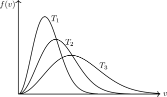
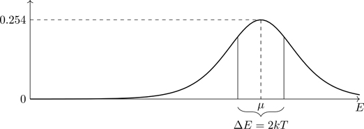
is the Maxwell speed distribution3,4,5 for v≥0, the probability f(v)dv of finding a particle with speed between v and v+dv. We cited the Maxwell distribution as an example of a probability density function in Eq. (3.27). Equation (5.5) shows there is a distribution in molecular speeds in a gas in equilibrium at temperature T—a big conceptual discovery by Maxwell.6 A gas in thermal equilibrium—seemingly a quiescent system—actually consists of a collection of molecules having a range of speeds: a few slow ones, a few fast ones, with most having speeds near the mean.7 The shape of the distribution is shown in Fig. 5.1. The speed distribution confirms our physical expectation that as the temperature is lowered, progressively more of the molecules have slower speeds. We’ll see that such an expectation can fail when quantum mechanics is brought into account.
Figure 5.1Maxwell speed distribution f(v) for T1<T2<T3. The area under the curve is the same for each temperature.
We can calculate the mean speed using the rules of probability,
v¯=∫0∞vf(v)dv=8kTmπ.
(5.6)
There are other ways, however, to characterize the speed of atoms in a gas. What’s the “rms” (root-mean-square) speed? By definition,
vrms=v2¯=∫0∞v2f(v)dv1/2=3kTm.
(5.7)
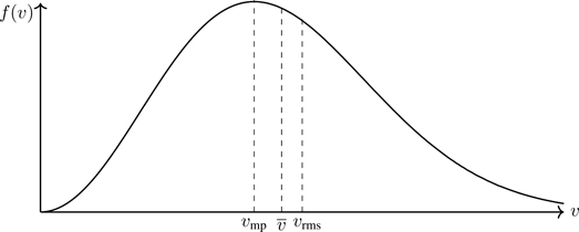
Note that we don’t actually need to do the integral in Eq. (5.7); it follows from the equipartition theorem (Section 4.1.2.11), 〈mv2/2〉=(3/2)kT —why the factor of 3? We can also ask for the most probable speed vmp at which the distribution has a maximum. This is readily found to have the value
Figure 5.2Characteristic molecular speeds of a gas in thermal equilibrium: vmp, v¯, vrms.
Example. Nitrogen is the largest component of air (approximately 78%, with oxygen comprising 21%).8 What is the mean speed v¯ of a nitrogen molecule at room temperature, T=293 K, given that nitrogen occurs as a diatomic molecule N2 at this temperature? To apply Eq. (5.6), we need the molecular mass. The mass number of a nitrogen atom is approximately 14 grams/mole (consult a periodic table of the elements, 14.007 when isotopic variances are taken into account). The mass of the molecule is therefore 28 grams/mole; Avogadro’s number of N2 molecules has a mass of 28 grams. The mass of one molecule is therefore m=28g/(6.02×1023)=4.65×10−23g=4.65×10−26 kg. Using Eq. (5.6), we find v¯=471 m/s. That’s fast! The speed of a bullet fired from a gun is ≈500 m/s. Keep in mind that Eq. (5.5) is a distribution of speeds, not velocities. In equilibrium, the molecules of a gas have their velocities directed at random, implying the net velocity is zero. Table 5.1 lists the mean speed v¯ for various gases at room temperature.
Table 5.1 Mean speed v¯ of selected gases at T=293 K
Some of the most successful applications of statistical mechanics involve the magnetic properties of materials. Under the general banner of magnetism there are different types of magnetic phenomena: ferromagnetism, antiferromagnetism, paramagnetism, diamagnetism, and others. In the limited space of this book we can only offer a cursory treatment of the subject. Ferro- and antiferromagnetism are cooperative effects produced by interactions among the magnetic dipoles of the atoms in a solid. Paramagnetism is the “ideal gas” of magnetism, in which magnetic moments interact only with an applied magnetic field and not with each other.
For a collection of magnetic moments {μi} that interact only with the external field, we need treat only the statistical mechanics of a single magnetic moment. The partition function for N identical, noninteracting particles ZN=(Z1)N, where Z1 is the single-particle partition function. The energy of interaction between a magnetic dipole moment μ and a magnetic field9B is E=−μ·B.
Should we adopt a classical or a quantum treatment of this problem? It turns out that a quantum treatment leads to excellent agreement with experimental results. Thus, we consider the energy of interaction between μ and B as the Hamiltonian operator,
H^=−B·μ^=gμBℏB·J^=gBμBℏJ^z,
(5.9)
where we’ve used Eq. (E.4), μ=−gμBJ/ℏ, where μB≡eℏ/(2m) is the Bohr magneton, g is the Land e´ g-factor (see Appendix E), and the operator J^z is the z-component of the total angular momentum (the B-field defines the z-direction). To use Eqs. (4.123) or (4.125) (quantum statistical mechanics in the canonical ensemble), we require the eigenfunctions and eigenvalues of the Hamiltonian operator, which in this case is proportional to J^z (Eq. (5.9)). As is well known, J^2 and J^z have a common set of eigenfunctions |J,m〉 (a complete orthonormal set), such that
J^2|J,m〉=J(J+1)ℏ2|J,m〉J^z|J,m〉=mℏ|J,m〉,
where the quantum number J has the values J=0,1,2,⋯ or J=12,32,52,⋯, and m=−J,−J+1,⋯,J−1,J so that there are (2J+1) values of m. The energy eigenvalues are therefore Em=gμBmB. From Eq. (4.123),10
Z1=∑m=−JJe−βmμBgB=sinhy(J+12)sinhy/2,
(5.10)
where y≡βμBgB. The summation in Eq. (5.10) is simple because it’s a finite geometric series.
To calculate the average value of11μz, we use Eq. (4.125), (where |m〉≡|J,m〉)
By evaluating the derivative indicated in Eq. (5.11), we find, after some algebra,
〈μz〉=μBgJBJ(βμBgBJ),
(5.12)
where BJ(x) is the Brillouin function of order J, defined as
BJ(x)≡2J+12Jcoth2J+12Jx−12Jcoth12Jx.
(5.13)
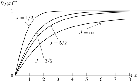
Graphs of these functions are shown in Fig. 5.3. They demonstrate the characteristic feature of saturation, that limx→∞BJ(x)=1 for all J. At a fixed temperature, for increasing values of the magnetic field, μ becomes (on average) progressively more aligned with the direction of the field. For strong enough fields, the moments are ostensibly all aligned with the field; increasing the field further can only keep the moments at their maximum alignment with the field—saturation.
Figure 5.3Brillouin functions BJ(x) for J=1/2,3/2,5/2, and J=∞.
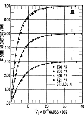
Figure 5.4 shows measured values of 〈μz〉 as a function of B/T at several values of T for three paramagnetic salts which contain an ion for which g=2, but for which the values of J are different, J=32,52,72. The data are presented as 〈μz〉/μB, which, from Eq. (5.12), because g=2, saturate at the values of 3, 5, 7, precisely what is found experimentally. Furthermore, the data fall almost perfectly on the Brillouin functions, validating the predictions of Eq. (5.12).
Figure 5.4Plot of 〈μz〉/μB versus B/T for three paramagnetic ions. The solid lines are the predictions of Eq. (5.12). Curve I is for potassium chromium alum ( J=32,g=2), curve II is for iron ammonium alum ( J=52,g=2), and curve III is for gadolinium sulfate octahydrate ( J=72,g=2). Reprinted figure with permission from W.E. Henry, Phys. Rev. 88, p.559 (1952).[48] Copyright (2020) American Physical Society.
Another measured quantity is the magnetic susceptibility,
χ≡(∂M∂H)|H=0,
(5.14)
where M is the magnetization, M=N〈μz〉. To calculate the susceptibility, we could differentiate the Brillouin function BJ(x) and let x→0, but that’s an unnecessary step. Using the result of Exercise 5.9, combined with Eq. (5.12), and setting B=μ0H, we have for small H,
M~H→0N3kT(μBg)2J(J+1)μ0H≡CHT,
(5.15)
where
C=N3kμ0μBg2J(J+1).
(5.16)
Equation (5.15), Curie’s law, is the equation of state of a paramagnet—the magnetization is linear with H for small M. The constant C is the Curie constant, the value of which is material specific.12 From Eq. (5.15), as H→0, M→0, the hallmark of paramagnetism—the system acquires a magnetization in an applied magnetic field, which vanishes in zero field.13 For small fields, the larger the susceptibility, the larger is the magnetization obtained for the same field strength.
Paramagnetism can be treated classically if we consider the magnetic moment a vector (not an operator): μ=μe^, where e^ is a unit vector that can point in any direction. The energy E=−μBcosθ, where θ is the angle between B and μ. We use Eq. (4.15) for the partition function, Z=∫e−βEΩ(E)dE. The density of states function Ω(E) is found by differentiating the formula E(θ)=−μBcosθ, implying Ω(θ)=sinθ. (We leave off the factor of μB to keep the density of states dimensionless, the number of states in the range [θ,θ+dθ]). Thus,
Z=∫0πeβμBcosθsinθdθ=2βμBsinh(βμB).
(5.17)
To obtain the average value of μz, we use Eq. (5.11),
〈μz〉=∂∂(βB)lnZ=μL(x),
(5.18)
where x≡βμB and L(x) is the Langevin function,
L(x)≡cothx−1x.
(5.19)
From Exercise 5.9, L(x) is the limiting form of BJ(x) as J→∞.
No physics book can be complete without treating the harmonic oscillator, as it’s among the few exactly solved problems in physics. We’re fortunate this problem can be solved exactly, because it occurs widely in physics. For a potential energy function V(r) that has a minimum at r=r0, its Taylor series about r0 is V(r)=V(r0)+(r−r0)dV/dr|r0+12(r−r0)2d2V/d2r|r0+…. If the system is in equilibrium at r=r0 (no force acting), dV/dr|r0=0, and assuming d2V/dr2|r0>0 (stable equilibrium), then small excursions about r=r0 map onto the harmonic oscillator with mω2≡d2V/dr2|r0. In what follows, assume we have a harmonic oscillator of mass m and angular frequency ω in equilibrium with a heat bath at temperature T. We consider the problem from the quantum and the classical perspectives.
5.3.1 Quantum treatment
Harmonic oscillators have quantized energy levels14En=(n+12)ℏω, n=0,1,2,⋯. The energy associated with n=0, 12ℏω, is the zero-point energy, the lowest possible energy that a quantum system may have (which, we note, is not zero).15 The canonical partition function for a single oscillator is, from Eq. (4.123),16
Z1(β)=∑n=0∞e−β(n+12)ℏω=12sinh(βℏω/2).
(5.20)
The partition function specifies the number of states a system has available to it at temperature T. As β→0 (high temperature), we have from Eq. (5.20),
Z1(β)~β→01βℏω,
(5.21)
that all of the infinite number of energy states of the harmonic oscillator become thermally accessible, that Z diverges as we (formally) allow T→∞. Compare with the β→0 limit of the partition function for a paramagnetic ion, Eq. (5.17), Z(β→0)=2. In that case there are only two states available to the system: aligned or antialigned with the direction of the magnetic field. Consider the other limit of Eq. (5.20),
Z1(β)~β→∞e−βℏω/2.
(5.22)
For temperatures such that kT≲ℏω/2, Z1≪1; the number of states available to the system is exponentially smaller than unity. As T→0 there are no states available to the system: Z→0.
Applying Eq. (5.20) to Eq. (4.40), we have the average energy of the oscillator,
〈E〉=ℏω2coth12βℏω=ℏω1eβℏω−1+12≡ℏω〈n〉+12.
(5.23)
Let’s look at the limiting forms of Eq. (5.23):
〈E〉=ℏω2(T→0)〈E〉=kT.(T→∞)
(5.24)
At low temperature, the system occupies its ground state, with energy E=ℏω/2. At sufficiently high temperatures, the system behaves classically, with energy given by the equipartition theorem. We’ve written Eq. (5.23) in the form 〈E〉=(〈n〉+12)ℏω, where 〈n〉 denotes the occupation number specifying the effective average state that the system is “in” (or occupies) in thermal equilibrium,
〈n〉=1eβℏω−1.
(5.25)
The occupation number 〈n〉 is not an integer. The system (oscillator) is continually exchanging energy with its environment, causing it to momentarily occupy the allowed states of the system labeled by integer n. The occupation number is the average value in thermal equilibrium of the quantum number n. We can either say that the system has energy 〈E〉=(〈n〉+12)ℏω, or, equivalently (because the energy of an ideal system is the sum of the energies of its components), that the system consists of 〈n〉quantara17 each of energy ℏω.
We note that Eq. (5.25) is the Bose-Einstein distribution function for bosons with μ=0 (see Eq. (5.61)), which is also the Planck distribution for the number of thermally excited photons of energy E=ℏω (see Section 5.8.2). Is there a connection between bosons and harmonic oscillators? There is indeed, as we now show.18
For a system of N independent oscillators, the partition function ZN(β)=Z1(β)N. Thus, using Eq. (5.20),
ZN(β)=2sinh(βℏω/2)−N=e−Nβℏω/21−e−βℏωN.
(5.26)
Equation (5.26) is a closed-form expression for the partition function of N independent harmonic oscillators, from which one could calculate the heat capacity—see Eq. (5.41). We can, however, express Eq. (5.26) in another way. Apply the binomial theorem Eq. (3.10) to Eq. (5.26):
ZN(β)=e−Nβℏω/2∑k=0∞(N+k−1k)e−kβℏω.
(5.27)
Writing ZN(β) in the form of Eq. (4.15) (the Laplace transform of the density of states), ZN(β)=∫0∞ΩN(E)e−βEdE, we infer from Eq. (5.27) that the density of states for N independent harmonic oscillators has the form
ΩN(E)=∑k=0∞(k+N−1k)δ(E−(k+N/2)ℏω),
(5.28)
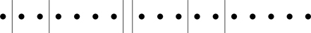
where δ(x) is the Dirac delta function. What combinatorial problem does the binomial coefficient N+k−1k pertain to? Consider, starting from N oscillators each in its ground state (so E=Nℏω/2 is the zero-point energy of the system), how many ways can k quanta, each of energy ℏω, be added to N oscillators so that the energy of the system is E=(k+N/2)ℏω ? Quanta are indistinguishable; we can’t say which quantum of energy is added to an oscillator, all we can say is that k quanta have been added to the system. The combinatorial problem is therefore how many distinct ways can k indistinguishable quanta be added to Ndistinguishable oscillators? Figure 5.5 shows 17 “dots,” where the dots represent energy quanta, distributed among 7 oscillators, where the oscillators have been conceptually arranged in a line, separated by vertical lines. N oscillators are delineated by (N−1) vertical lines. There would be (N+k−1)! permutations of the (N+k−1) symbols in Fig. 5.5, but that would overcount the number of distinct configurations of the system. We should divide (N+k−1)! by k! for permutations of the k dots, and by (N−1)! for permutations of the oscillators. Thus, the number of distinct permutations of k dots among the N−1 lines is k+N−1k.
Figure 5.5One of the k+N−1k ways of distributing k indistinguishable energy quanta (shown here as 17 identical dots) among N oscillators (shown here as 7 boxes, delineated by 6 vertical lines). In this example, a box in the middle has no quanta.
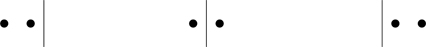
Example. There are 32=3 ways of adding k=2 quanta to N=2 oscillators; see Fig. 5.6.
Figure 5.6The three distinct configurations of two quanta added to two oscillators.
5.3.2 Classical treatment
The Hamiltonian function for the harmonic oscillator is H=p2/(2m)+12mω2x2, implying
Z1(β)=1h∫−∞∞dx∫−∞∞dpe−β[p2/(2m)+12mω2x2]=1βℏω.
(5.29)
Planck’s constant enters the evaluation of Z in classical statistical mechanics (see Section 2.3). The partition function for the quantum harmonic oscillator in the high-temperature limit is the same as that for the classical oscillator.
In Section 5.1, we treated the ideal gas of structureless molecules, the most salient feature of which is the translational kinetic energy of its point particles. Translational motion is present in any gas. The constituents of real gases have internal motions that we have yet to take into account. We consider the ideal diatomic gas,19 i.e., we ignore inter-particle interactions and we assume the conditions for classical behavior apply, nλT3≪1 (see Section 1.11). It should be clear that internal motions must be treated using quantum mechanics—classical statistical mechanics brings with it the equipartition theorem, which we know is insufficient to explain the heat capacity of real gases.
Energies of translational degrees of freedom and those of internal motions can be written in terms of individual Hamiltonians,
H=Htrans+Hrot+Hvib+Helec+⋯,
(5.30)
where Htrans is the Hamiltonian associated with translational motion, Hrot is that for rotations, Hvib for vibrations, Helec for electronic degrees of freedom, and so on. Writing H in this form assumes the degrees of freedom underlying each Hamiltonian are noninteracting, that the various modes of excitation occur independently—an approximation that’s not always true. When H can be written in separable form, the partition function occurs as the product of the partition functions associated with each part of the Hamiltonian:20
Z(T,V)=1N!Ztrans(T,V)·Zrot(T)·Zvib(T)·….
(5.31)
In that case, the heat capacity occurs as the sum of the heat capacities for each of the modes of excitation (because CV is related to lnZ; see Exercise 4.14):
CV(T)=Ctrans+Crot(T)+Cvib(T)+⋯.
(5.32)
For an ideal gas, Ctrans=32Nk is independent of temperature.21 In this section, we calculate the heat capacities for the rotational and vibrational degrees of freedom of the ideal diatomic gas.
5.4.1 Rotatonal motion
The rigid rotor problem treats the two atoms of a diatomic molecule as having a fixed separation distance r0. The allowed rotational energies depend on the moment of inertia I=μr02, where μ is the reduced mass of the two atomic masses, μ=m1m2/(m1+m2). The rotational state is determined by the angular momentum operator, L^. L^2 and L^z have a common set of eigenfunctions,
L^2|l,m〉=l(l+1)ℏ2|l,m〉L^z|l,m〉=mℏ|l,m〉,
where l=0,1,2,⋯ and m=−l,−l+1,⋯,l−1,l so that there are 2l+1 values of m. The Hamiltonian for rotational motion about the center of mass is H^rot=L2/(2I), and thus the rotational energy eigenvalues are El=ℏ2l(l+1)/(2I). Because El is independent of the quantum number m, each state is (2l+1)-fold degenerate. The partition function is, using Eq. (4.123),22
Z1,rot(T)=∑l=0∞(2l+1)e−βEl.
(5.33)
The sum in Eq. (5.33) cannot be evaluated in closed analytic form, and we must introduce approximations. We examine the high and low-temperature limits.
5.4.1.1High-temperature form
As β→0 there are contributions to Eq. (5.33) from large values of the quantum number l, which suggests we approximate the sum in Eq. (5.33) with an integral, using the form of Z in Eq. (4.15). That route requires the density-of-states function, Ω(E), the derivative with respect to energy of the total number of energy states up to and including E. Energy at a specified value E implies a maximum value of l determined by E=ℏ2lmax(lmax+1)/(2I)≈ℏ2lmax2/(2I) because lmax≫1. How many states are there for 0≤l≤lmax ? It can be shown that
∑l=0lmax(2l+1)=lmax+12≈lmax2≈2Iℏ2E.
(5.34)
The density of states is therefore Ω(E)=2I/ℏ2. Thus, we can approximate Eq. (5.33),
Z1,rot(T)=2Iℏ2∫0∞e−βEdE=2Iβℏ2≡TΘr,(T≫Θr)
(5.35)
where Θr=ℏ2/(2Ik) sets a characteristic temperature for rotational motions.23 Using equations that we’ve now used several times (Eqs. (4.40) and (P4.1)), with Z=(Z1)N,
〈E〉rot=NkTCVrot=Nk,(T→∞)
(5.36)
the same as what we obtain from the equipartition theorem.
A more accurate high-temperature form can be obtained using the result of Exercise P5.2:
Z1,rot(T)=TΘr+13+115ΘrT+4315ΘrT2+⋯.(T≫Θr)
(5.37)
From Eq. (5.37) we obtain an expression for the heat capacity more general than Eq. (5.36) (see Exercise 5.12),
CV(T)rot=Nk1+145ΘrT2+16945ΘrT3+⋯.(T≫Θr)
(5.38)
We see that (CV(T))rot exceeds the classical value Nk, a value that it tends to as T→∞.
5.4.1.2Low-temperature form
In the low-temperature regime, T≪Θr, we have, from Eq. (5.33),
Z(T)1,rot=1+3e−2Θr/T+5e−6Θr/T+⋯.
(5.39)
In this case, the variable e−Θr/T is exponentially small as T→0. From Eq. (5.39), we find to lowest order
CV(T)rot≈12NkΘrT2e−2Θr/T.(T≪Θr)
(5.40)
As T→0, CV(T)rot drops to zero exponentially fast; rotational degrees of freedom can’t be excited at sufficiently low temperature—they become “frozen out.”
The two equations, (5.38) and (5.40), are limiting forms of CV(T)rot in the high- and low-temperature regimes. They each show that the heat capacity is temperature dependent. To obtain the complete temperature dependence of CV(T)rot requires the use of a computer to evaluate the sum in Eq. (5.33) at each temperature. A detailed analysis shows there is a maximum value of CV(T)rot≈1.1Nk at T≈0.81Θr. Given that Θr≈10 K, measurements of CV on diatomic gases at room temperature are consistent with the prediction of the equipartition theorem.
5.4.2 Vibrational motion
The partition function for the quantum harmonic oscillator is given in Eq. (5.20), from which may be derived an expression for the heat capacity,
CV(T)vib=NkΘvT2eΘv/TeΘv/T−12,
(5.41)
where Θv≡ℏω/k is a characteristic temperature associated with vibrational energies. For HCl, Θv≈4300 K, and for H2, Θv≈6300 K. Thus, only for temperatures on the order of 104 K would we expect vibrational modes to be sufficiently excited that they contribute to CV at the level required by the equipartition theorem. From Eq. (5.41) we have the high and low-temperature limits:
CVvib=Nk(T≫Θv)CVvib~NkΘvT2e−Θv/T.(T≪Θv)
(5.42)
Given that Θv~103 K, vibrational modes are frozen out at room temperature and don’t appreciably contribute to CV.
We now take into account the indistinguishability of identical particles required by quantum mechanics. We start with the Hamiltonian for a system of N noninteracting identical particles, H^=∑n=1Nh^n, where h^n is a function of the coordinates and momenta associated with an isolated atom or molecule, which can include the translational motion of the center of mass or the degrees of freedom associated with rotation, vibration, intra-atomic electronic structure, and the intrinsic spin, S. The energy of an ideal system is the sum of the energies of its constituents, E=∑n=1NE(n), where E(n) is the energy of the nth particle, which is any one of the eigenvalues belonging to h^. (We don’t have to label h^ with an index—it’s the same function for all particles.) The quantity E(n) is a function of the quantum numbers associated with the aforementioned degrees of freedom, such as the wavevector k introduced in Section 2.1.5, rotational or vibrational quantum numbers, or the z-component of the spin. We denote the collection of relevant quantum numbers associated with the nth particle as mn. Thus, E(n)=E(n)(mn).
5.5.1 Partition function
We might assume that the canonical partition function can be written in the form
ZN=∑m1⋯∑mNexp−β∑n=1NE(n).(wrong!)
(5.43)
Equation (5.43) is incorrect because it overcounts the allowed states of identical particles. The occupation numbernk is the number of particles in the system having the eigenstate associated with eigenvalue Ek (see Appendix D). The energy of the system can therefore be written not as a sum over particles, as in E=∑n=1NE(n), but as a sum over energy levels,
E=∑mnmEm.
(5.44)
Equation (5.44) is an important step in setting up the statistical mechanics of identical particles. The occupation numbers must satisfy the constraint
∑mnm=N.
(5.45)
Equations (5.44) and (5.45) are unrestricted sums over all possible energy states.24
How many ways can the energy E be partitioned over the particles of the system? For a given set of occupation numbers {nk} satisfying Eq. (5.45), there are, using Eq. (3.12), N!/∏k(nk!) ways of permuting the particles, which, by the indistinguishability of identical particles, are equivalent and have to be treated as a single state. To correct for overcounting, Eq. (5.43) should be written
ZN=1N!∑m1⋯∑mN∏k(nk!)exp−β∑n=1NE(n).
(5.46)
Equation (5.46) presents a challenging combinatorial problem because it connects the energy levels of individual particles, E(n), to the occupation numbers nk, which apply to the entire system. To apply Eq. (5.46), we must know the occupation numbers associated with a system in thermal equilibrium, which is what we’re trying to solve for! At high temperature (β→0) the number of energy levels that can make a significant contribution to the sum in Eq. (5.46) becomes quite large. One would expect, for fixed values of N and E, that in this limit the occupation numbers will be predominately 0 or 1 and thus (nk)!=1 for most configurations. If we set (nk)!=1 in Eq. (5.46), we have an approximate expression for the partition function (which factorizes)
where in the last step we’ve used that all particles are identical, where Z1 is the partition function for a single particle. Equation (5.47) is the high-temperature limit of the partition function for bosons or fermions.
It was noted in Section 1.11 that for combinations of temperature and density such that nλT3≳1, the boson or fermion character of the particles of the system must be taken into account. We’ll see in Section 5.5.3 how this criterion emerges from a calculation of the equation of state.25 We consider an ideal gas of point particles in the absence of an external magnetic field, so that the relevant quantum numbers26 are the wavevector k associated with the particle’s kinetic energy (see Eq. (2.14)) and its spin quantum number σ. The energy eigenvalues in this case27 are
Ek,σ=Ek=ℏ22mk2,
(5.48)
where the eigenvalues are g-fold degenerate, with g=2S+1. It’s shown in Appendix D how, in creating wavefunctions displaying the proper symmetries under permutations of particles, that information about particle identity is lost. We can’t say which particle has a given energy, because of the indistinguishability of identical particles. The most we can say is how many particles have a given energy (the occupation number), and not which particles have that energy. We can therefore write the N-particle partition function, not as in Eq. (5.46) (a sum over particles), but in the form
ZN=∑{nk,σ}∑k,σnk,σ=Ne−β∑k,σnk,σEk,σ,
(5.49)
a sum over energy levels, where ∑{nk,σ} denotes a summation over all quantum numbers (k,σ), ∑{nk,σ}≡∏k,σ∑k,σ. Equation (5.49) indicates, for each allowed (k,σ), to sum over the occupation numbers nk,σ, subject to the constraint ∑k,σnk,σ=N.
Equation (5.49) is in general impossible to evaluate, because of the constraint of a fixed number of particles, Eq. (5.45). One has a formidable combinatorial problem of summing over all sets of occupation numbers consistent with the constraint on the number of particles. Without the constraint, Eq. (5.49) would simply factorize. Surprisingly, this problem simplifies in the grand canonical ensemble where, by allowing N to vary, the constraint is eliminated. Referring to Eq. (4.127),
where now the sums over occupation numbers are unrestricted. The transition from Eq. (5.50) to Eq. (5.51) can be shown by the method of staring at it long enough. Consider a system that has only two energy levels, E1 and E2. In that case, we would have from Eq. (5.50)
ZG=∑N=0∞∑n1(n1+n2=N)∑n2eβ(μ−E1)n1+β(μ−E2)n2
(5.52)
Let a≡eβ(μ−E1) and b≡eβ(μ−E2), so that Eq. (5.52) can be expressed
ZG=∑N=0∞∑n1=0N∑n2=0N−n1an1bn2.
Write out the first few terms in the series: For N=0, a0b0=1; for N=1, a0b1+a1b0=a+b; for N=2, a2+ab+b2; and for N=3, a3+a2b+ab2+b3. Add these terms (up to and including N=3):
ZG=(1+b+b2+b3)+a(1+b+b2)+a2(1+b)+a3(1).
We see the pattern: As N→∞, we have the unrestricted sums,
ZG=∑n1=0∞∑n2=0∞an1bn2=∑n1=0∞an1∑n2=0∞bn2.
Generalize to a set of k energy levels E1,E2,⋯,Ek, with ai≡eβ(μ−Ei), i=1,⋯,k. Then, from Eq. (5.50),
the same as Eq. (5.51) when we let k→∞. With Eq. (5.51) established, we can quickly complete the calculation.
The occupation numbers of fermions are restricted to the values n=0,1 for any state (the Pauli principle). In that case, we have from Eq. (5.51)
ZG(β,μ)=∏k,σ1+eβ(μ−Ek,σ).(F)
(5.53)
For bosons there are no restrictions on the occupation numbers. The sum in Eq. (5.51) can be evaluated explicitly as a geometric series, with the result
ZG(β,μ)=∏k,σ11−eβ(μ−Ek,σ).(B)
(5.54)
For the infinite series to converge requires that μ≤0 for bosons. There is no restriction on μ for fermions. These formulas can be combined into a common expression. Let θ=+1 for bosons and θ=−1 for fermions (the same factor of θ introduced in Eq. (4.110)). Equations (5.53) and (5.54) can then be written as a common expression
ZG(β,μ)=∏k,σ1−θeβ(μ−Ek,σ)−θ.(θ=±1)
(5.55)
The partition function for the ideal quantum gas thus factorizes, but the factors don’t pertain to individual particles—they refer to individual energy levels.
5.5.2 The Fermi-Dirac and Bose-Einstein distributions
The average number of particles a system has (associated with given values of μ,T,V —we’re using the grand canonical ensemble) can be found from the derivative (see Eq. (4.78))
〈N〉=kT∂lnZG∂μT,V.
Using Eq. (5.55) for ZG,
∂lnZG∂μ|T,V=gβ∑k1eβ(Ek−μ)−θ,
(5.56)
where g=2S+1 is the spin degeneracy (see Eq. (5.48)). Thus,
〈N〉=g∑k1eβ(Ek−μ)−θ.
(5.57)
The sum in Eq. (5.57) can be converted to an integral over k-space, ∑k⟶(V/(8π3))∫d3k (see Section 2.1.5),
where, because for free particles Ek is isotropic in k-space (see Eq. (5.48)), we work in spherical coordinates. Change variables28 in Eq. (5.58); let E=ℏ2k2/(2m). Then,
where we’ve used the free-particle density of states, g(E), Eq. (2.18), and where we’ve introduced the average occupation numbers,
〈n〉θ=1eβ(E−μ)−θ.(θ=±1)
(5.60)
The functions implied by Eq. (5.60) for θ=±1 are called the Bose-Einstein distribution function ( θ=1),
〈n〉BE=1eβ(E−μ)−1,
(5.61)
and the Fermi-Dirac distribution function ( θ=−1),
〈n〉FD=1eβ(E−μ)+1.
(5.62)
For fermions, 0<〈n〉FD≤1, which (as we’ll discuss) reflects the requirements of the Pauli principle. There is no restriction on 〈n〉BE (other than 〈n〉BE>0) because μ≤0 for bosons. These functions (Eqs. (5.61) and (5.62)) are fundamental to any discussion of identical bosons or fermions. We’ve derived them from the partition function in the grand canonical ensemble, the appropriate ensemble if the chemical potential is involved. There’s another method, however, for deriving these functions that’s often presented in textbooks, the method of the most probable distribution, shown in Appendix F.
The structure of Eq. (5.59) is a generic result in statistical mechanics:
〈N〉=∫0∞g(E)n(E)dE.
(5.63)
The average number of particles is obtained from a sum over energy levels, with the density of states g(E) telling us the number of allowed states per energy range, multiplied by n(E), the average number of particles occupying those states in thermal equilibrium. One is from quantum mechanics—the allowed states of the system, the other is from statistical physics, the number of particles actually occupying those states in equilibrium at temperature T and chemical potential μ.
5.5.3 Equation of state, fugacity expansions
From Eq. (4.76), Φ=−kTlnZG. For a system with V as the only relevant external parameter, Φ=−PV, Eq. (4.69). For such a system, PV=kTlnZG. Using Eq. (5.55) for ZG, we have the equation of state:
PV=−θgkT∑kln1−θeβ(μ−Ek).
(5.64)
The sum in Eq. (5.64) can be converted to an integral, ∑k⟶(V/(8π3))∫d3k (see Section 2.1.5). Thus,
PV=−θgkTV8π3∫d3kln1−θeβ(μ−Ek).
(5.65)
Because Ek is isotropic in k-space, work with spherical coordinates:
PV=−gθkTV8π3∫0∞4πk2dkln1−θeβ[μ−ℏ2k2/(2m)].
Change variables: Let x≡βℏ2k2/(2m), a dimensionless variable. Then,
P=−gθkTλT32π∫0∞dxxln1−θeβμ−x.
Integrate by parts:
P(T,μ)=gkTλT31Γ(5/2)∫0∞x3/2ex−βμ−θdx.
(5.66)
Note that Eq. (5.66) provides an expression for P that’s intensive in character; P=P(T,μ) is independent of V. Pressure P, which has the dimension of energy density, is equal to kT, an energy, divided by λT3, a volume, multiplied by a dimensionless function of eβμ (the integral in Eq. (5.66)).
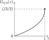
The two equations implied by Eq. (5.66) (one for each of θ=±1) involve a class of integrals known as Bose-Einstein integrals for θ=1, Gn(z), defined in Eq. (B.18), and Fermi-Dirac integrals for θ=−1, Fn(z), defined in Eq. (B.29), where z=eβμ. Written in terms of these functions, we have from Eq. (5.66),
P(T,μ)=gkTλT3{G5/2(z)θ=+1F5/2(z)θ=−1.
(5.67)
Because for bosons 0<z≤1, an expansion in powers of z can be developed for Gn(z), a fugacity expansion (see Eq. (B.21)). For fermions there is no restriction on z (only that z>0). A fugacity expansion can be developed for Fn(z) for 0<z≤1 (see Eq. (B.32)); for z≫1, one has to rely on asymptotic expansions (see Eq. (B.40)), or numerical integration.
Using Eqs. (B.21) and (B.32) for the small-z forms of Gn(z),Fn(z), we have from Eq. (5.67),
P=gkTλT3z1+θz25/2+z235/2+θz345/2+⋯.(θ=±1)
(5.68)
For the classical ideal gas, the chemical potential is such that z=eβμ=nλT3 (see Eq. (P1.3)). In the classical regime, nλT3≪1, implying classical behavior is associated with z≪1. Ignoring the terms in square brackets in Eq. (5.68), we recover the equation of state for the classical ideal gas, P=nkT (the degeneracy factor g “goes away,” for reasons we explain shortly). Fugacity is a proxy for pressure (see page 100), and we see from Eq. (5.68) that z∝P in the classical limit.
From Eqs. (5.66) or (5.68) we have the pressure in terms of μ and T. The chemical potential, however, is not easily measured, and P is more conveniently expressed in terms of the density n≡N/V. It can be shown using Eqs. (5.59), (B.18), and (B.29), that
N(T,V,μ)=gVλT3{G3/2(z)θ=+1F3/2(z)θ=−1.
(5.69)
From Eq. (5.69) and Eqs. (B.21) and (B.32), we find a fugacity expansion for the density:
λT3gn=z1+θz23/2+z233/2+θz343/2+⋯.
(5.70)
We can invert the series in Eq. (5.70) to obtain z in terms of a density expansion.29 Working consistently to terms of third order, we find
z=λT3ng1−θ23/2λT3ng+14−133/2λT3ng2+⋯.
(5.71)
When nλT3≪1, the terms in square brackets in Eq. (5.71) can be ignored, leaving us (in this limit) with z=nλT3/g, a generalization of what we found from thermodynamics, Eq. (P1.3), to include spin degeneracy. Thus, from Eq. (5.68), P=nkT in the classical limit.
Substitute Eq. (5.71) into the fugacity expansion for the pressure, Eq. (5.68). We find, working to third order,
P=nkT1+a1θλT3ng+a2λT3ng2+⋯
(5.72)
where
a1=−123/2=−0.1768a2=−235/2−18=−0.0033.
A density expansion of P (as in Eq. (5.72)) is called a virial expansion. For classical gases, the terms in a virial expansion result from interactions between particles (see Section 6.2). The terms in square brackets in Eq. (5.72) are a result of the quantum nature of identical particles and not from “real” interactions. That is, nominally noninteracting quantum particles act in such a way as to be effectively interacting. The requirements of permutation symmetry imply a type of interaction between particles—because of Eq. (4.110), correlations exist among nominally noninteracting particles, a state of matter not encountered in classical physics. We see from Eq. (5.72) that the pressure of a dilute gas of fermions (bosons) is greater (lesser) than the pressure of the classical ideal gas. The Pauli principle effectively introduces a repulsive force between fermions: Configurations of particles in identical states occupying the same spatial position do not occur in the theory, as if there was a repulsive force between particles. For bosons, it’s as if there’s an attractive force between particles.
5.5.4 Thermodynamics
We can now consider the other thermodynamic properties of ideal quantum gases. From Eq. (4.82),
where we’ve used Eq. (5.55). Using the same steps as in previous sections, we find
U(T,V,μ)=32gVλT3kT{G5/2(z)θ=+1F5/2(z)θ=−1.
(5.74)
Equation (5.74) is quite similar to Eq. (5.67), which we may use to conclude that
U=32PV⇒P=23UV.
(5.75)
Equation (5.75) holds for all ideal gases, which is noteworthy because the equations of states of the classical and two quantum ideal gases are different.30
To calculate the heat capacity, it’s useful31 to divide Eq. (5.74) by Eq. (5.69):
where primes indicate a derivative with respect to z, and where (shown in Exercise 5.14)
∂z∂T|n=−32zTA3/2(z)A1/2(z).
(5.78)
Combining Eqs. (5.78) and (5.77), and making use of Eqs. (B.20) and (B.31), we find
CVNk=154A5/2(z)A3/2(z)−94A3/2(z)A1/2(z).
(5.79)
Equation (5.79) applies for fermions and bosons. It’s easy to show, using either Eq. (B.21) or (B.32) that as z→0, CV→Nk(154−94)=32Nk, the classical value. We’ll examine the low-temperature properties in upcoming sections.
An efficient way to calculate the entropy is to use the Euler relation, Eq. (1.53),
S=1TU+PV−Nμ=1T53U−Nμ=Nk52A5/2(z)A3/2(z)−lnz,
(5.80)
where we’ve used Eqs. (5.75) and (5.76) and the definition of z=eβμ. (See Exercise 5.15.) The form of Eq. (5.80) for small z is, using Eqs. (B.21) and (B.32) and Eq. (5.71) at lowest order,
S=Nk52−lnλT3ng,(z≪1)
a generalization of the Sackur-Tetrode formula to include spin degeneracy (see Eq. (1.64)).
Equation (5.75) allows an easy way to calculate the heat capacity in the regime nλT3≪1, without the heavy machinery of Eq. (5.79). From
CV=∂U∂TV=32∂(PV)∂TV=32Nk1−12a1θnλT3g−2a2nλT3g2
(5.81)
where we’ve used Eq. (5.72). Putting in numerical values,
CV=32Nk1+0.0884θnλT3g+0.0066nλT3g2⋯.
(5.82)
As T→∞, CV approaches its classical value, 32Nk. For bosons ( θ=+1) the value of CV for large but finite temperatures, is larger than the classical value, implying that the slope of CV versus T is negative, which a calculation of ∂CV/∂T from Eq. (5.82) shows. We know that heat capacities must vanish as T→0, a piece of physics not contained in Eq. (5.82), a high-temperature result.
As Eqs. (5.72) and (5.82) show, there are minor differences between the two types of quantum gases in the regime nλT3≪1, with the upshot that the two cases can be treated in tandem (as we’ve done in Sections 5.5.3 and 5.5.4). We now consider the opposite regime (nλT3)/g≳1 in which quantum effects are more clearly exhibited, in which Fermi and Bose gases behave differently, and which must be treated separately.
We start with the Fermi gas, which is simpler. At a given temperature, particles distribute themselves so as to minimize the energy.32 Our expectation is that as the temperature is lowered, progressively more of the lower-energy states become occupied (such as we see in Fig. 5.1). Because of the Pauli principle, however, fermions cannot accumulate in any energy level, which, as a consequence, implies that at low temperature the lowest-energy configuration of a system of noninteracting fermions is to have one particle in every energy level, starting at the lowest possible energy, with all energy levels filled until the supply of particles is exhausted. The energy of the top-most-occupied state (technically at T=0) is the Fermi energy, EF, the zero-point energy of a collection of noninteracting fermions. This is the most important difference between Fermi and Bose gases. The state of matter in which all the lowest energy states of the system are occupied is called degenerate. Particles of a degenerate Fermi gas occupy states of high kinetic energy at low temperature.33 The degeneracy parameter
δ≡nλT3g=ngh3(2πmkT)3/2
(5.83)
distinguishes systems in which quantum effects are small ( δ≪1) from those in which there are strong quantum effects ( δ≳1).34
5.6.1 Identical fermions at T=0
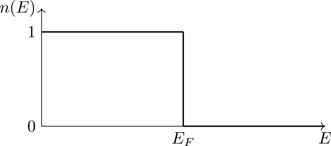
In the limit T→0, the Fermi factor becomes a step function,35
n(E)=1eβ(E−μ)+1→T→0{1E<EF0E>EF≡θ(EF−E),
(5.84)
where EF≡μ(T=0) is the zero-temperature limit36 of the chemical potential, and θ(x) is the Heaviside step function, θ(x)≡{0x<01x>0, the graph of which is shown in Fig. 5.7.
Figure 5.7The Fermi-Dirac distribution at T=0. States for which E<EF are all occupied ( n=1) and states for which E>EF are all unoccupied ( n=0).
The Fermi energy is easy to calculate. Combining Eq. (5.84) with Eq. (5.59),
The energy of the “last” particle added to the system, EF, is therefore the chemical potential of the N-particle system—the energy required to add one more particle. From Eq. (5.86), we see that the higher the density, the larger the Fermi energy—adding more particles to the same volume requires progressively higher and higher energy levels to be filled. Equation (5.86) implies an equivalent temperature associated with particles at the Fermi energy, the Fermi temperature, TF defined so that kTF=EF,
TF=ℏ22mk6π2gn2/3.
(5.87)
It should not be construed that particles actually have the Fermi temperature (the temperature here is T=0); TF is a convenient way to characterize the Fermi energy.
The Fermi energy can be quite large relative to other energies. Table 5.2 lists the density n of free electrons (those available to conduct electricity37) for selected elements in their metallic states, together with the value of EF as calculated from Eq. (5.86) using g=2 for electrons ( S=12). We can associate with EF an equivalent speed known as the Fermi velocity, vF≡2EF/m. The Fermi velocity is the speed of an electron having energy EF. Compare such speeds ( ≈106 m/s at metallic densities) with thermal speeds in gases at room temperature, ≈500 m/s (see Table 5.1). That vF can be so large (at zero temperature) is a purely quantum effect—as more particles are added to the same volume, they must occupy progressively higher energy levels because of the Pauli principle, which at metallic densities are ≈5 eV. The thermal equivalent of 1 eV is 11,600 K (show this), implying TF≈50,000 K. For sufficiently large densities—such as occur in astrophysical applications—fermions would have to be treated relativistically (see Section 5.7). Electron densities in metals ( n≈1022 cm-3) should be compared with the densities of ordinary gases. At standard temperature and pressure (STP), T=273.15 K and P=1 atm, the density of the ideal gas is n≈2.7×1019 cm-3.
Table 5.2 Electron densities, Fermi energies, velocities, and temperatures of selected metallic elements. Source: N.W. Ashcroft and N.D. Mermin, Solid State Physics[18].
Element
n (1022 cm-3)
EF (eV)
vF (106 m s-1)
TF (104 K)
Li
4.70
4.74
1.29
5.51
Na
2.65
3.24
1.07
3.77
K
1.40
2.12
0.86
2.46
Rb
1.15
1.85
0.81
2.15
Cs
0.91
1.59
0.75
1.84
Cu
8.47
7.00
1.57
8.16
Ag
5.86
5.49
1.39
6.38
Au
5.90
5.53
1.40
6.42
Another way to calculate EF is to work in k-space (see Section 2.1.5). Associated with the Fermi energy is a wavevector, the (you guessed it) Fermi wavevectorkF such that
ℏ22mkF2≡EF.
(5.88)
Between Eqs. (5.88) and (5.86),
kF=6π2gn1/3.
(5.89)
The Fermi wavevector therefore probes a distance d~n−1/3=(V/N)1/3, the distance between particles. As the density increases, the distance between particles decreases, and kF increases.
The Fermi wavevector defines a surface in k-space, the Fermi surface, a sphere of radius kF (the Fermi sphere), that separates filled from unfilled energy states, depicted in Fig. 5.8. Each allowed k-vector is uniquely associated with a small volume of k-space, 8π3/V (Section 2.1.5). Each k-vector (representing solutions of the free-particle Schrödinger equation satisfying periodic boundary conditions) is associated with g=2S+1 energy states, when spin degeneracy is accounted for. The number of particles N in the lowest-energy state,38 those with k-vectors lying within the Fermi sphere, can be found from the number of allowed k-vectors interior to the Fermi surface, multiplied by g:
N=g(4π/3)kF3(8π3/V)=gV6π2kF3,
(5.90)
Figure 5.8The Fermi sphere separates states occupied for k≤kF and unoccupied for k>kF. Third dimension not shown.
a calculation that reproduces Eq. (5.89).
What is the energy of the ground-state configuration? Is it EF? From Eq. (5.73) it can be shown that
U=∫0∞Eg(E)n(E)dE.
(5.91)
Equation (5.91) has a similar structure to Eq. (5.63): The average energy of the system is given by an integral over the density of states g(E) (number of allowed states per energy range), multiplied by the average number of particles occupying those states in thermal equilibrium n(E) (either the Fermi-Dirac or Bose-Einstein distributions), multiplied by the energy, the quantity we’re trying to find the average of. Combining Eq. (5.84) with Eq. (5.91),
Thus, the average energy per particle (at T=0) is 35 of the Fermi energy. That implies the mean speed per particle is 3/5vF≈0.77vF. The pressure of the Fermi gas can be found by combining Eq. (5.75) with Eq. (5.93):
P=23UV=23UNNV=25nEF=ℏ25m6π2g2/3n5/3.
(5.94)
Because of its large zero-point energy, the Fermi gas has a considerable pressure39 at T=0. Equation (5.94) specifies the degeneracy pressure of the Fermi gas at T=0. Can the degeneracy pressure be measured? The bulk modulusB is the inverse of the isothermal compressibility,
B≡−V∂P∂VT=25nEF=53P,
(5.95)
where we’ve used Eq. (5.94). (Note that for the classical ideal gas, B=P.) Table 5.3 lists values of B as calculated from Eq. (5.95) and measured values. The agreement is satisfactory, but even when the predictions are considerably off, it gets you on the same page as the data. The degeneracy pressure alone can’t explain the bulk modulus of real materials, but it’s an effect at least as important as other physical effects. The degeneracy pressure underscores that the Pauli principle in effect introduces a repulsive force between identical fermions, a rather strong one. Note that nowhere have we brought in the electron charge—the predictions of this section would apply equally as well for a collection of neutrons. Why the Fermi gas model works so well for electrons in solids was something of a puzzle when the theory was developed by Sommerfeld in 1928. Coulomb interactions between electrons would seemingly invalidate the assumptions of an ideal gas. The answer came only later, in the development of Fermi liquid theory (beyond the scope of this book). In solids, electrons screen the positive charges of the ions that remain on the lattice sites of a crystalline solid, after each atom donates a few valence electrons to the lattice. As a result, electrons in metals act as almost-independent “quasiparticles,” a topic we won’t develop in this book.
Table 5.3 Bulk modulus (Gpa) of selected elements in their metallic states. Source: N.W. Ashcroft and N.D. Mermin, Solid State Physics[18].
Element
B (Eq. (5.95))
B (expt)
Li
23.9
11.5
Na
9.23
6.42
K
3.19
2.81
Rb
2.28
1.92
Cs
1.54
1.43
Cu
63.8
134.3
Ag
34.5
99.9
Al
228
76.0
5.6.2 Finite-temperature Fermi gas, 0<T≪TF
For T≠0, we can no longer use the “easy” equations (5.87) and (5.92). Instead we must use Eqs. (5.69) and (5.74), which, for arbitrary temperatures, must be handled numerically. At sufficiently low temperatures, however, deviations from the results at T=0 are small, and we can approximate Eqs. (5.63) and (5.91) appropriately. Of course, we have to quantify what constitutes low temperature, which, as we’ll see, are temperatures T≪TF. Because TF can be rather large (for metallic densities), one often has systems for which room temperature can be considered “low temperature.”
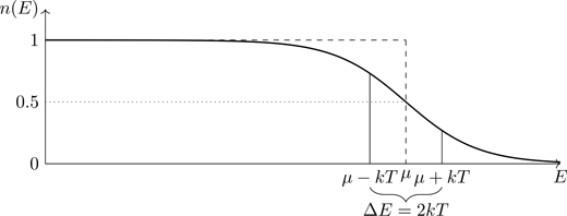
Figure 5.9 shows the Fermi-Dirac distribution at finite temperature. We see a softening of the characteristic sharp edge between occupied and unoccupied states that occurs for T=0 (see Fig. 5.7). States at E=μ−kT are not all occupied ( n(E)<1), and states at E=μ+kT are not all unoccupied ( n(E)>0). The temperature used to make Fig. 5.9 is such that kT=0.1μ, which is actually quite large (for systems of metallic density). Such a temperature was chosen so that the features of the Fermi distribution could be easily discerned in a figure such as Fig. 5.9. For a more realistic temperature such as kT=0.01μ, the transition region of approximate energy width ΔE≈2kT would occur over a smaller energy range and be more difficult to display.
Figure 5.9The Fermi-Dirac distribution at finite temperature (solid line). Dashed line corresponds to T=0. Temperature was chosen so that kT=0.1μ.
Referring to Fig. 5.9, the unoccupied states for energy μ−αkT (where α is a number) occur as a result of transitions induced by thermal energies 2αkT to occupy states of energy μ+αkT. We expect that the heat capacity of a system of fermions (the ability to absorb energy) would therefore be controlled by states occurring within an approximate energy range kT of μ. We’ll see that’s indeed the case (see Eq. (5.106)). For n(E) the average number of states occupied at energy E, its complement (1−n(E)) is the average number of unoccupied states at energy E. Unoccupied states are referred to as holes. The product of the two, n(E)1−n(E), is largest for energies at which particles and holes are both prevalent. As is readily shown:
n(E)1−n(E)=eβ(E−μ)eβ(E−μ)+12.
(5.96)
Figure 5.10Product n(E)(1−n(E)) of the number of occupied states and the number of holes (unoccupied states) versus E. Note change in vertical scale from Fig. 5.9. kT=0.1μ.
Note that the right side of Eq. (5.96) (plotted in Fig. 5.10) is an even function40 of E−μ.
5.6.2.1Chemical potential
Referring to Eq. (5.63), at low temperatures, kT≪μ, i.e., βμ≫1, the Fermi distribution transitions from 1 to 0 over a narrow energy range about E=μ. Under these circumstances there exists a method for accurately approximating integrals such as we have in Eq. (5.63), the Sommerfeld expansion, Eq. (B.49). Using Eq. (5.69),
where t≡T/TF. The quantity y in Eq. (5.100) must vanish as T→0. Noting that n varies with temperature in Eq. (5.100) (for fixed μ) as powers of t2, let’s guess that y is a function of t2 as well (for small t). Let y=at2+bt4+⋯ where a and b are dimensionless constants, to be determined. Keeping terms to second order in small quantities, we have from Eq. (5.100),
n(t)n0=1+t2π28+32a+t47π4640−π216a+32b+38a2+⋯.
(5.101)
Let’s find solutions of Eq. (5.101) at fixed density, which we take to be the zero-temperature value, n0 (which asserts itself through the value of EF, or TF). With that assumption, setting n(t)=n0, the terms in square brackets in Eq. (5.101) must vanish, implying a=−π2/12 and b=−π4/80. Thus,
μ(n,T)=EF1−π212TTF2−π480TTF4+⋯,
(5.102)
where the density dependence is implicit through the value of TF. For T≪TF, we can treat systems as if the temperature is T=0.
The chemical potential for a system of fermions decreases for T>0. As the temperature is raised from T=0, particles are promoted to states of energies E>EF. We note that μ is, from the definition of the Fermi-Dirac distribution, the energy of the state for which the average occupation number n(E=μ)=0.5if μ>0. As particles are promoted to higher-lying states, μ must shift downward—the state for which n(E)=0.5 occurs at a smaller energy. As the temperature is increased so that T≲TF, a detailed analysis shows that μ→0, implying that the state for which n(E)=0.5 occurs at E=0. At even higher temperatures, μ becomes negative. To see this, consider the value of n(E=0)=e−βμ+1−1. One has, for any value of βμ, n(E=0)<1, and we know that for T≪TF, n(E=0) is almost unity, e−βEF+1−1. One can show that if μ>0, then n(E=0)>12. To have n(E=0)<12, it must be the case that μ<0, at which point μ loses its interpretation as the energy for which n(E)=0.5. For μ<0, we have that the limiting form of the Fermi factor for T→∞ is n(E)=12 for all E—the average value of n(E)=0.5 for every state; every state is either occupied or unoccupied with equal probability in the extreme high-temperature limit.
5.6.2.2Internal energy
Starting from Eq. (5.74) and using the Sommerfeld expansion, Eq. (B.49), we find
Divide Eq. (5.103) by Eq. (5.97); we find, working to second order,
UN=35μ1+π221(βμ)2−11π41201(βμ)4+⋯.
(5.104)
By substituting Eq. (5.102) into Eq. (5.104) and working consistently to second order, we find
UN=35EF1+5π212TTF2−5π480TTF4+⋯.
(5.105)
Equation (5.105) is the finite-temperature generalization of Eq. (5.93).
5.6.2.3Heat capacity
Using Eq. (5.104) we can calculate the heat capacity,
CV=∂U∂TV,N=Nkπ22TTF−3π420TTF3+⋯.(T≪TF)
(5.106)
Clearly, CV vanishes as T→0 (compare with Eq. (5.82)). We also see a characteristic feature of the Fermi gas: CV is linear with T at low temperature.
One can understand CV∝T at low temperature qualitatively.42 As per the considerations leading to Eq. (5.96), the energy states that can participate in energy transfers between the system and its environment are those roughly within kT of μ, which at low temperature is ostensibly the Fermi energy, EF. How many of those states are there? The number of energy states per energy range is the density of states, g(E). Thus, g(EF)×kT is approximately the number of states near EF available to participate in energy exchanges, and is therefore the number of states that contribute to the heat capacity.43 The excitation energy for each energy transfer is approximately kT. Thus, we can estimate the energy of the Fermi gas at low temperatures as
U≈U0+g(EF)×kT×kT,
where U0=35NEF, Eq. (5.93). As shown in Exercise 5.19, g(EF)EF=32N. The heat capacity based on this line of reasoning would then be
CV≈2k2g(EF)T=3NkTTF.
Such an argument gets you on the same page with the exact result, Eq. (5.106); the two differ by a multiplicative factor of order unity, π2/6.
Degeneracy pressure, associated with the large zero-point energy of collections of identical fermions, accounts reasonably well for the bulk modulus of metals (Section 5.6)—that compressing an electron gas meets with a significant resisting force associated with the Pauli exclusion principle. In this section we consider an astrophysical application of degeneracy pressure.
Stars generate energy through nuclear fusion, “burning” nuclei in processes that are fairly well understood. Stars convert hydrogen to helium by a series of fusion reactions: H1+H1→H2+e++ν, H2+H1→He3+γ, He3+He3→He4+H1+H1. When all hydrogen has been converted to helium, this phase of the burning process stops. Gravitational contraction then compresses the helium until the temperature rises sufficiently that a new sequence of reactions can take place, He4+He4→Be8+γ, Be8+He4→C12+γ. As helium is exhausted, gravitational contraction resumes, heating the star until new burning processes are initiated. The variety of nuclear processes gets larger as new rounds of nuclear burning commence (the subject of stellar astrophysics). Eventually burning stops when the star consists of iron, silicon, and other elements. The force of gravity, however, is ever present. Can gravitational collapse can be forestalled? We now show that the degeneracy pressure of electrons in stars is enough to balance the force of gravity under certain circumstances.
We assume temperatures are sufficiently high that all atoms in stars are completely ionized, i.e., stars consist of fully-ionized plasmas, gases of electrons and positively charged species. Let there be N electrons (of mass m) and assume conditions of electrical neutrality, that N=Np, the number of protons (of mass mp). Assume that the number of neutrons Nn (locked up in nuclei) is the same as the number of protons, an assumption valid only for elements up to Z≈20; for heavier nuclei there might be ≈1.5 neutrons per proton. We take Nn=Np to simplify the analysis. The neutron mass is nearly equal to the proton mass. The mass M of the star is then, approximately (because mp≫m),
M≈Nm+2mp≈2Nmp.
(5.107)
We make another simplifying assumption that the mass density ρ=M/V is uniform44 throughout a star of volume V. With these assumptions, the average electron number density n≡N/V is
n=NV=M/(2mp)M/ρ=ρ2mp.
(5.108)
White dwarfs are a class of stars thought to be in the final evolutionary state wherein nuclear burning has ceased and the star has become considerably reduced in size through gravitational contraction, where a star of solar mass M⊙ might have been compressed into the volume of Earth. Sirius B, for example, is a white dwarf of mass 1.018M⊙ and radius 8.4×10⁻³R⊙, implying an average electron density 7.2×1029 cm-3, some seven orders of magnitude larger than the electron density in metals (see Table 5.2). We can take n=1030 cm-3 as characteristic of white dwarf stars. Such high densities necessitate a relativistic treatment of the electrons (see Exercise 5.20).
Before delving into a relativistic treatment of the electron gas, let’s calculate the gravitational pressure, for which we use classical physics. Assuming the mass density of a spherical star of radius R is uniform, the contribution to the gravitational potential energy from a spherical shell of matter between r and r+dr is (do you see Gauss’s law at work here?),
dVg=−G(4πr2drρ)(4πr3ρ/3)r=−G16π23ρ2r4dr.
Thus, the gravitational potential energy of a uniform, spherical mass distribution of radius R is
Vg=−G16π215ρ2R5=−35GM2R=−1254π31/3Gmp2N2V−1/3,
where it’s a good habit in these calculations to display the dependence on the number of electrons N and the volume V. The gravitational pressure, Pg, is found from
Pg≡−∂Vg∂VN=−454π31/3Gmp2N2V−4/3.
(5.109)
We have a negative pressure; gravity is an attractive force.
The question is: Under what conditions can the degeneracy pressure balance the gravitational pressure? Can we reach for Eq. (5.94), the previously-derived expression for the degeneracy pressure? We can’t—Eq. (5.94) was derived using the density of states for solutions of the Schrödinger equation (see Section 2.1.5). For the electron densities of white dwarf stars, the formulas derived in Section 5.6.1 imply Fermi velocities in excess of the speed of light; a relativistic treatment is called for. If you examine the arguments in Sections 5.5.1 and 5.5.2, in the derivation of the Fermi-Dirac and Bose-Einstein distributions, the specific form of the energy levels is not invoked, i.e., whether or not the energy levels are solutions of the Schrödinger equation. The distribution functions for occupation numbers require no modification for use in relativistic calculations. The density of states function, however, must be based on the allowed energy levels of relativistic electrons, which are found from the solutions of the Dirac equation. It would take us too far afield to discuss the Dirac equation, but we can say the following. The solutions of the free-particle, time-independent Schrödinger equation are in the form of plane waves, ψ~eik·r, with the wave vector related to the energy through E=ℏ2k2/(2m). The solutions of the Dirac equation (which pertains to non-interacting particles) are in the form of traveling plane waves,45ψ~eik·r−ωt where ω≡E/ℏ and k=p/ℏ are connected46 through the relativistic energy-momentum relation
E2=(pc)2+(mc2)2.
(5.110)
We’ve repeatedly invoked the replacement Σk→(V/(8π)3)∫d3k in converting sums over allowed energy levels (parameterized by their association with the points of k-space permitted by periodic boundary conditions) to integrals over k-space. Does it hold for relativistic energy levels? Yes, periodic boundary conditions can be imposed on the solutions of the Dirac equation and thus the enumeration of states in k-space proceeds as before, with one modification: The energy associated with k=0 is mc2 and not simply zero as in the nonrelativistic case. Moreover, there are two linearly independent solutions of the Dirac equation for wave vectors k satisfying Eq. (5.110),47 and thus g=2. We can calculate kF as previously, N=2∑|k|≤kF=2V8π3∫0kF4πk2dk=V3π2kF3, implying
kF=3π2n1/3,
(5.111)
equivalent to Eq. (5.90) with g=2. To find the Fermi energy, we would seemingly proceed as in Section 5.6.1: Substitute Eq. (5.111) into Eq. (5.110),
EF=mc21+ℏmc3π2n1/32.(wrong!)
(5.112)
Equation (5.112) implies, for n=1030 cm-3, EF=0.796 MeV, quite a large energy. In relativity theory, the zero of energy is the rest energy, mc2, as we see from Eq. (5.110). In what follows, we’ll use the kinetic energy T≡E−mc2 (not the temperature), the difference between the total energy and the rest energy. It’s the kinetic energy that’s involved in finding the pressure. We define
EF≡mc21+ℏmc3π2n1/32−1.
(5.113)
The dimensionless group of terms in Eq. (5.113), (ℏ/(mc))(3π2n)1/3, occurs frequently in the theory we’re about to develop; let’s give it a name, x≡(ℏ/(mc))(3π2n)1/3. For n=1030 cm-3, x=1.194, and Eq. (5.113) predicts EF=0.285 MeV. The temperature equivalent of 0.285 MeV (the Fermi temperature) is 3.3×10⁹ K. In comparison, the temperature of white dwarf stars is 10,000−20,000 K. We’re justified therefore in treating the electron gas as if it was at zero temperature! Equation (5.113) reduces to the nonrelativistic Fermi energy, Eq. (5.88), for x≪1:
EF=ℏ22m3π2n2/31+OλC/λF2,
(5.114)
where λC≡h/(mc) is the Compton wavelength, and λF≡2π/kF is the Fermi wavelength.48 The low-density limit is equivalent to λF≫λC. It can be shown that the inverse of Eq. (5.113) is
3π2n=1(ℏc)3EF2+2EFmc23/2.
(5.115)
5.7.1 Relativistic degenerate electron gas
We must develop the density of kinetic-energy levels for relativistic electrons. From Eq. (5.110),
where sinhθF≡EF2+2EFmc2/(mc2)=(ℏ/(mc))(3π2n)1/3≡x (where we’ve used Eq. (5.115)). The nonrelativistic limit EF≪2mc2 is therefore x≪1. The integral in Eq. (5.121) takes some algebra to evaluate. We find50
Compare the structure of Eq. (5.122) with Eq. (5.74); U is extensive (scales with V) but it’s also an energy. We see the ratio of V to λC3, the cube of the Compton wavelength, multiplied by an energy, mc2, whereas in Eq. (5.74) we have the ratio V/λT3 multiplied by kT.
The integrated part vanishes. In the remaining integral, let the temperature go zero, and let the Fermi factor provide the cutoff at k=kF:
P=13π2∫0kFk3dEkdkdk.
Change variables: Let Ek=T+mc2 and use Eq. (5.116),
P=13π21(ℏc)3∫0EFT2+2Tmc23/2dT.
Change variables again, using Eq. (5.119): We have, for the degeneracy pressure,
P=8π3mc2λC3∫0θFsinh4θdθ.
(5.123)
Once again we see that pressure is an energy density, mc2/λC3; compare with Eq. (5.66), where the pressure is related to another energy density, kT/λT3. Equation (5.123) presents us with another tough integral.51 We find (where x=sinhθF=(ℏ/(mc))(3π2n)1/3),
P=π3mc2λC3x(2x2−3)1+x2+3sinh−1x≡π3mc2λC3g(x).
(5.124)
Equation (5.124) is the equation of state for the degenerate electron gas as a general function of x=(ℏ/(mc))(3π2n)1/3. We can identify the two limiting forms (see Exercise 5.40),
We can use Eqs. (5.122) and (5.124) to form the ratio U/(PV) (see Exercises 5.39 and 5.40):
UPV=3f(x)g(x)={3/2x≪13x≫1.
(5.126)
5.7.2 White dwarf stars
We’ve now developed the machinery to address the question we posed earlier: Can the degeneracy pressure of electrons P balance the gravitational pressure, Pg? Under what conditions is P≥|Pg| ? Using Eq. (5.109) and the strong relativistic form of Eq. (5.125), we require
ℏc4(3π2)1/3N4/3V−4/3≥454π31/3Gmp2N2V−4/3.
The volume dependence is the same on both sides of the inequality; we therefore have a criterion on the number of electrons involving fundamental constants of nature:
N≤5169π41/3ℏcGmp23/2=1.024×1057.
A star has the same number of protons (electric neutrality), and by assumption the same number of neutrons. The mass of a star with N=1.024×1057 electrons is, from Eq. (5.107),
Equation (5.127) would specify the theoretical maximum mass of a star that can hold off gravitational collapse if the assumptions we’ve made are all accurate. We’ve used the strong relativistic form of Eq. (5.125) for x≫1, whereas for stars with electron concentrations of 1030 cm-3, x=1.194. A more drastic assumption is that the star consists of a fully-ionized plasma. The basic theory of the upper mass of white dwarf stars was developed by S. Chandrasekhar in the 1930s.52 When the degree of ionization is properly taken into account, the upper mass in Eq. (5.127) is revised downward. Detailed investigations by Chandrasekhar led to 1.44M⊙ as the upper bound, the Chandrasekhar limit.
5.7.3 Neutron stars
A star with mass in excess of the Chandrasekhar limit therefore cannot hold off gravitational collapse, right? Yes and no: Yes, the electron gas has a degeneracy pressure insufficient to balance the force of gravity, and no, because a new fusion reaction sets in. At sufficiently high pressures, the reaction e−+p→n+ν takes place, fusing electrons and protons into neutrons.53 The neutrinos escape; degenerate matter is transparent to neutrinos, leaving a neutron star. Neutrons are fermions and therefore have a degeneracy pressure. Neutrons, however, because they are so much more massive than electrons, can be treated nonrelativistically. The question becomes, under what conditions can the neutron degeneracy pressure exceed the gravitational pressure. Using the nonrelativistic form of P from Eq. (5.125), we have the inequality
ℏ25mn(3π2)2/3N5/3V−5/3≥154π31/3Gmn2N2V−4/3,
where N refers to the number of neutrons, and we’ve used the neutron mass, mn. This inequality is equivalent to
R≤ℏ2mn3G9π42/3N−1/3=1.31×1023N−1/3m,
(5.128)
where V1/3=(4π/3)1/3R specifies a radius R. For a neutron star of two solar masses, N=2.4×1057, in which case the critical radius R≈10 km! Nonrelativistic neutrons therefore have a degeneracy pressure sufficient to hold off gravitational collapse. If, however, as gravity compresses the star the neutrons are heated to such an extent that they “go relativistic,” there is no counterbalance to the force of gravity, and a black hole forms.
Photons are special particles: spin-1 bosons of zero mass that travel at the speed of light54 and have two spin states.55 They have another property that’s directly relevant to our purposes: Photons in thermal equilibrium have zero chemical potential, μ=0. Electromagnetic radiation is not ordinarily in equilibrium with its environment,56 implying it can’t ordinarily be described by equilibrium statistical mechanics. Cavity radiation, however, is the singularly important problem of electromagnetic energy contained within a hollow enclosure bounded by thick opaque walls maintained at a uniform temperature, and thus is in equilibrium with its environment. In this section, we apply the methods of statistical physics to cavity radiation.
5.8.1 Why is μ=0 for cavity radiation?
The assignment of μ=0 to cavity radiation can be established in thermodynamics. Consider the electromagnetic energy U contained within a cavity of volume V that’s surrounded by matter at temperature T. Denote the energy density as u(T)≡U(T)/V. Cavity radiation is independent of the specifics of the cavity—the size and shape of the cavity or the material composition of the walls—and depends only on the temperature of the walls. That conclusion follows from thermodynamics: Cavity radiation not independent of the specifics of the cavity would imply a violation of the second law[3, p68]. In particular, “second-law arguments” show that the density of electromagnetic energy is the same for any type of cavity and depends only on the temperature. Thus, we have “line one” for cavity radiation:
∂u∂VT=0.
(5.129)
Equation (5.129) is the analog of Joule’s law for the ideal gas, Eq. (1.44), ( ∂U/∂VT=0). Cavity radiation is not an ideal gas (see Table 5.4), even though both systems are collections of non-interacting entities. For the ideal gas, ΔU=0 in an isothermal expansion, i.e., U is independent of V. For cavity radiation, the energy density is independent of volume, with ΔU=uΔV in an isothermal expansion.57 The number of atoms in a gas is fixed, and heat absorbed from a reservoir in an isothermal expansion keeps the temperature of the particles constant. In an isothermal expansion of cavity radiation, heat is absorbed from a reservoir, but goes into creating new photons to keep the energy density fixed.
The equation of state for cavity radiation58 is[3, p70]
P=13u(T).
(5.130)
Compare with the equation of state for ideal gases, P=23u, Eq. (5.75). Equation (5.130) follows from an analysis of the momentum imparted to the walls of the cavity based on the isotropy of cavity radiation (another conclusion from second-law arguments59), that photons travel at the same speed, independent of direction, and that the momentum density of the electromagnetic field60 is u/c. With Eq. (5.130) established, using the methods of thermodynamics it can be shown that[3, p70]
u(T)=aT4,
(5.131)
where a is a constant, the radiation constant, the value of which cannot be obtained from thermodynamics. We’ll derive the value of this constant using statistical mechanics; see Eq. (5.140).
Once we know Eq. (5.131), we know a great deal. Combining Eq. (5.131) with Eq. (5.130),
P=a3T4.
(5.132)
The radiant energy in a cavity of volume V at temperature T is, from Eqs. (5.131) and (5.129),
U=aVT4.
(5.133)
The heat capacity is therefore
CV=∂U∂TV=4aVT3.
(5.134)
Note that CV(T)→0 as T→0, as required by the third law of thermodynamics. From Eq. (5.134), we can calculate the entropy:
∂S∂TV=1TCV⇒S=43aVT3.
(5.135)
With Eqs. (5.132), (5.133), and (5.135) (those for P, U, and S), we have the ingredients to construct the thermodynamic potentials:
The Gibbs energy is identically zero, a result obtained strictly from thermodynamics. In general, G=Nμ, Eq. (1.54). Because G=0 for cavity radiation for any N, we infer μ=0, implying it costs no extra energy to add photons to cavity radiation (but of course it costs energy to make photons). Photons are a special case in that creating them is the same as adding them to the system.61
Now that we’ve brought it up, however, what is the number of photons in a cavity? Thermodynamics has no way to calculate that number. Can we use the formalism already developed, say Eq. (5.69), to calculate the average number of photons? Not directly: The thermal wavelength λT=h/2πmkT depends on the mass of the particle; moreover the formulas derived in Section 5.5 for bosons utilize the density of states of nonrelativistic particles, Eq. (2.17). To calculate the number of photons, we must start over with Eq. (5.63) using the density of states for relativistic particles; see Eq. (2.20). Thus, with g=2 and μ=0,
Between Eqs. (5.133), (5.135), and (5.137), we have
SN=2aπ23ζ(3)ℏck3UN=aπ22ζ(3)ℏck3T.
(5.138)
For cavity radiation, therefore, S is strictly proportional to N, S∝N. For the ideal gas (see Eq. (1.64)), S~N, but is not strictly proportional to N. From the definition of the chemical potential, Eq. (1.22),
μ≡∂U∂NS,V,
we see that one can’t take a derivative of U with respect to N holding S fixed, because holding S fixed is to hold N fixed (what is (∂f/∂x)x ?). It’s not possible to change the number of photons keeping entropy fixed, and thus chemical potential is not well defined for cavity radiation.
We arrived at that conclusion, however, assuming μ=0. Is the assignment of μ=0 for cavity radiation consistent with general thermodynamics? From Table 1.2, ΔFT,V=W′, the amount of “other work.” Using Eq. (5.136), ΔFT,V=0. The maximum work in any form is ΔFT (see Section 1.5), and from Eq. (5.136), ΔFT=−13aT4ΔV=−PΔV, where we’ve used Eq. (5.132). Thus, no forms of work other than PdV work are available to cavity radiation, which is consistent with μ=0. Thermodynamic equilibrium is achieved when the intensive variables conjugate to conserved quantities (energy, volume, particle number) equalize between system and surroundings (see Section 1.12). Photons are not conserved quantities. Photons are created and destroyed in the exchange of energy between the cavity walls and the radiation in the cavity. There’s no population of photons external to the cavity for which those in the cavity can come to equilibrium with. The natural variables to describe the thermodynamics of cavity radiation are T, V, S, P, or U, but not N. Cavity radiation should not be considered an open system, but a closed system that exchanges energy with its surroundings. The confusion here is that photons are particles of energy, a quintessential quantum concept. Table 5.4 summarizes the thermodynamics of the ideal gas and the photon gas.
Table 5.4 Thermodynamics of the ideal gas and the photon gas
Ideal gas
Photon gas
Internal energy
U=32NkT
U=aVT4
Volume dependence of U
∂U∂VT=0
∂u∂VT=0
Equation of state
P=NkT/V=23u
P=13aT4=13u
Heat capacity
CV=32Nk
CV=4aVT3
Entropy
S=Nk52+lnVNλT3
S=43aVT3
Chemical potential
μ=−kTlnVNλT3
μ=0
Adiabatic process
TVγ−1=constant
TV1/3=constant
5.8.2 The Planck distribution
With μ=0 established, it remains to ascertain the radiation constant a before we can say the thermodynamics of the photon gas is completely understood (see Table 5.4). Without statistical mechanics, the radiation constant would have been considered a fundamental constant of nature, akin to the gas constant, R. A perfect marriage of thermodynamics and statistical mechanics, we can calculate the internal energy U (combining Eqs. (5.91) and (2.20), with g=2 and μ=0) and compare with Eq. (5.133):
Equation (5.140) is one of the triumphs of statistical mechanics. Note that we can’t take the classical limit of the radiation constant by formally letting ℏ→0. There is no classical antecedent of cavity radiation; it’s an intrinsically quantum problem from the outset.62
Let u(λ,T) denote the energy spectral density, the energy per volume contained in the wavelength range (λ,λ+dλ) in equilibrium at temperature T. (Thus, u(λ,T) has the units J m-4; do you see why?) Starting from Eq. (5.139) and changing variables, E=hc/λ, we find
U=8πhcV∫0∞dλλ51exp(hc/(λkT))−1≡V∫0∞u(λ,T)dλ,
and therefore we identify
u(λ,T)=8πhc1λ51exp(hc/(λkT))−1.
(5.141)
Equation (5.141) is called (among other names) the Planck distribution law.63 By changing variables, λ=c/ν, we have the frequency distribution (see Exercise 5.32),
u(ν,T)=8πhc3ν3eβhν−1.
(5.142)
5.8.3 The Wien displacement law
We’ve written the energy spectral density function as u(λ,T) and u(ν,T) in Eqs. (5.141) and (5.142), indicating they are functions of two variables, (λ,T) or (ν,T). This isn’t correct, however. Wilhelm Wien showed, in 1893, that u(λ,T), presumed a function of two variables, is actually a function of a single variable, λT. He showed that the spectral density function must occur in the form
u(ν,T)=ν3ψνToru(λ,T)=1λ5f(λT),
(5.143)
where ψ and f are functions of a single variable, precisely in the forms of Eqs. (5.141) and (5.142). Wien didn’t derive the Planck distribution—Planck’s constant had not yet been discovered—but his work placed an important constraint on its possible form.64
Wien’s central result is a partial differential equation for u as a function of ν and V (see [3, pp73–78]):
V∂u(ν)∂VS=ν3∂u(ν)∂ν−u(ν).
(5.144)
Equation (5.144) follows from an analysis of the means by which u can change in a reversible, adiabatic process. As can readily be verified, the solution of Eq. (5.144) is in the form
u(ν)=ν3ϕ(Vν3),
(5.145)
where ϕ is any function of a single variable. The functional form of ϕ cannot be established by this means of analysis.65
In a reversible, adiabatic process ( dS=0), we have for cavity radiation that VT3=constant (see Table 5.4). Equation (5.145) can therefore be written (for cavity radiation)
u(ν,T)=ν3ϕν3T3≡ν3ψνT,
(5.146)
where ψ is a function of a single variable. From Eq. (5.146), we have under the change of variables ν=c/λ, using energy conservation u(ν)dν=u(λ)dλ,
u(λ,T)=dνdλu(ν)=c4λ5ψcλT≡λ−5f(λT).
(5.147)
If every dimension of a cavity is expanded uniformly, the wavelength of every mode of electromagnetic oscillation would increase in proportion—that is, there would be a redshift. For a length L≡V1/3 associated with the cavity, every wavelength λ scales with L, λ~L=V1/3, and, because TV1/3 is constant in an isentropic process, λT=constant, or, equivalently, ν/T=constant. We know that ∫0∞u(ν,T)dν=U/V=aT4. Assume that in an isentropic expansion the radiation temperature changes from T1→T2. Then, we have the equality
1T14∫0∞u(ν,T1)dν=1T24∫0∞u(ν′,T2)dν′.
(5.148)
Applying Wien’s result, Eq. (5.146), to Eq. (5.148),
∫0∞νT13ψνT1dνT1=∫0∞ν′T23ψν′T2dν′T2.
(5.149)
Equation (5.149) implies the Wien displacement law: Under the expansion, for every frequency ν for the system at temperature T1, there’s an associated (“displaced”) frequency ν′=(T2/T1)ν at temperature T2 (change variables in Eq. (5.149), ν/T1=ν′/T2). Wien’s law therefore implies that the form of the Planck distribution remains invariant in an isentropic expansion; one has to “displace” the frequencies ν→ν′=(T2/T1)ν. This finds applications in the subject of cosmology, where the expansion of the universe is modeled as an isentropic process.66
It’s clear that u(ν)→0 as ν→0 (as ν→0, λ→∞, and a cavity of finite size cannot support an infinite-wavelength mode of electromagnetic vibration). It’s also true that u(ν)→0 as ν→∞ (see Exercise 5.35). Mathematically, the energy spectral density u(λT) must have a maximum (Rolle’s theorem). Suppose the function f(λT) in Eq. (5.147) is known (which it is, from the Planck distribution). Its maximum with respect to λ is obtained by satisfying the condition xf′(x)=5f(x), where x≡λT (show this). The wavelength where maximum energy density occurs is
λmax=1T5ff′max≡bT,
(5.150)
where the quantity b is known as Wien’s constant; it has the value b=2.898×10⁻³ m K.
In Section 5.5 we looked at the thermodynamic properties of ideal gases of fermions or bosons, Eqs. (5.67), (5.69), (5.74), and (5.80), those67 for P, N, U, and S. These formulas require modification at low temperature for bosons. At low temperature, bosons occupy low-lying energy states with no limit on the number of particles that can occupy a given state.68 As T→0, nothing prevents all particles from occupying (condensing into) the lowest energy state, which we’ve taken to be at E=0. For bosons, E=0 is “where the action is” at low temperature.69 The density of states function, however, g(E)vanishes as E→0 (see Eq. (2.18)). Because g(E) pertains to single-particle states, one might question the assumption of noninteracting particles as T→0. Can we even speak of a gaseous state at absolute zero temperature? As we’ll see, if we can “fix up” the treatment of Bose gases to properly capture the special state associated with E=0, it leads to a fascinating piece of physics, the Bose-Einstein condensation, a new state of matter predicted in 1924 but not observed until 1995, which was the basis for the 2001 Nobel Prize in Physics.70
To see what the issue is, consider Eqs. (5.67) and (5.69) for bosons ( θ=1), which involve the Bose-Einstein functions G5/2(z) and G3/2(z). From Eq. (B.21),
G5/2(z)=∑m=1∞zmm5/2G3/2(z)=∑m=1∞zmm3/2.
Power-series representations are valid provided the series converge. The interval of convergence for both series is 0<z≤1; they diverge for z>1. The function G3/2 is plotted in Fig. 5.11 for 0≤z≤1; that for G5/2 has a similar shape. The integral representation of G3/2 is (see Eq. (B.18))
G3/2(z)=1Γ(3/2)∫0∞xz−1ex−1dx.
The denominator of the integrand vanishes when ex=z. For z>1, there exists a value of x>0 (i.e., within the range 0<x<∞) at which the integral diverges. The functions G3/2(z) and G5/2(z) do not exist for z>1. Mathematically, the fact that these functions have maximum values as z→1− lies at the root of the theory of Bose-Einstein condensation.71
Figure 5.11Bose-Einstein function G3/2(z). The slope becomes infinite as z→1−.
From Eq. (5.69) we have (where for simplicity we take g=1), nλT3=G3/2(z). For a fixed density, at sufficiently high temperatures nλT3 is small, and one has a solution of Eq. (5.69) for small72z. As the temperature is lowered (for fixed density) nλT3 increases in value, for which, referring to Fig. 5.11, there will be solutions of Eq. (5.69) for z<1. At a critical temperature, however, the “last” solution of Eq. (5.69) occurs for z=1, where73nλT3=ζ(3/2), at the temperature
TB≡ℏ22mk8π3ζ(3/2)n2/3.
(5.151)
Equation (5.151) defines the Bose temperature, TB. Aside from numerical factors of order unity, the Bose temperature is similar to the Fermi temperature, Eq. (5.87): ℏ2/2m, which from the Schrödinger equation has the dimension of energy-(length)2, multiplied by n2/3, which provides 1/(length2). The length in question, n−1/3, is the average distance between particles. Whereas the Fermi temperature associated with electrons at metallic densities is quite large (see Table 5.2), the Bose temperature is quite small because the mass m refers to that of atoms.74 There is no solution of Eq. (5.69) at fixed density for T<TB. Equation (5.151) specifies a density-dependent temperature at which nλTB3=ζ(3/2). The critical density, nc is such that ncλT3≡ζ(3/2),
nc=ζ(3/2)2πmkTh23/2.
(5.152)
At a given temperature, there is no solution to Eq. (5.69) for n>nc.
Example. Consider a gas of 6×10²² He4 atoms (one-tenth of a mole) confined to a volume of one liter. What is its Bose temperature, TB? He4 is a boson: Its nucleus consists of two protons and two neutrons. By the rules of angular momentum addition in quantum mechanics, the spin of a composite object of two spin- 12 particles is either 1 or 0, and is therefore a boson. Nature seeks the lowest energy configuration, which would be for two identical fermions to pair such that the net spin is zero (no Pauli exclusion effect and hence lower energy). The two electrons in He4 also pair such that their spins are oppositely directed: He4 is a boson of spin zero. (By this reasoning, is He3 a boson?) What’s the mass of a He4 atom? I hope you’re reaching for Avogadro’s number: 6.64×10⁻²⁷ kg. Using Eq. (5.151), we find TB=0.059 K. In everyday experience that’s an exceedingly small temperature, but one that’s routinely achievable in modern laboratories.75
What does a maximum density imply for the chemical potential? We have, from Eq. (5.69), z=eβμ=G3/2−1(nλT3), where G3/2−1 denotes the inverse function of G3/2. We don’t have an expression for G3/2−1, but we do have an analytic form for G3/2 valid for z≲1 that can easily be inverted, Eq. (B.23): G3/2(βμ)=ζ(3/2)−2π−βμ+O(−βμ), implying for T≳TB,
βμ≈−14πζ(3/2)−nλT32=−ζ(3/2)24π1−TBT3/22,
(5.153)
where we’ve used ζ(3/2)=nλTB3. Equation (5.153) can be written, to lowest order,
μkTB≈−CT−TBTB2,(T≳TB)
(5.154)
where C≡9ζ(3/2)2/(16π)≈1.22. Thus, μ vanishes as T→TB+, as shown in Fig. 5.12.
Figure 5.12Chemical potential of the ideal Bose gas for T≳TB (from Eq. (5.154)).
The upshot is that Eq. (5.69) is valid only for nλT3≤ζ(3/2), implying μ≤0 for T≥TB only.76 It’s as if at low temperatures, in approaching the maximum density nc, the extra particles we’re adding to the system (at fixed volume) simply “disappear.” Where did we go wrong? We went wrong in the transition from equations such as (5.57) and (5.64) to Eqs. (5.58) and (5.66), in converting sums over allowed states to integrals over k-space, in making the replacement ∑k→(V/8π3)∫d3k. The state associated with k=0 is given zero weight in the resulting integral, yet that state dominates the physics of bosons at low temperature. Let’s split off the k=0 state from the sum in Eq. (5.57), and then let ∑k→(V/8π3)∫d3k:
N=g1e−βμ−1︸N0, number of particles in the ground state+g∑k≠01eβ(Ek−μ)−1︸Nex,number of particles in excited states=gz1−z+gV8π3∫d3keβ(Ek−μ)−1=gz1−z+gVλT3G3/2(z)≡N0+Nex.
(5.155)
In Eq. (5.155), N0 denotes the number of particles in the ground state, with Nex the number of particles in all other, excited states of the system. The “missing” particles are in the ground state! This is the Bose-Einstein condensation: Starting at T=TB and continuing to T=0, particles begin occupying the ground state of the system with significant (macroscopic) numbers, until, at T=0, all particles of the system occupy the ground state.77 Equation (5.155) can be written (compare with Eq. (5.69)),
nλT3g=λT3Vz1−z+G3/2(z).
(5.156)
Henceforth we will set g=1 in formulas related to the Bose gas; experiments on Bose-Einstein condensation utilize atoms for which g=1.
As long as z≪1, the new term in Eq. (5.156) is negligibly small because of the factor of V−1, with the value of z implied by Eq. (5.156) not appreciably different from what we obtained from Eq.(5.69). When, however, z has a value infinitesimally close to z=1, which we can characterize as z≈1−O(N−1) (for macroscopic N), then the factor of z/(1−z) in Eq. (5.156) cannot be neglected. As z→1−, this term saves us from the apparent missing-particle “trap” set by Eq. (5.69)—there is no longer a maximum density of Bose gases. Indeed, we can find a solution for z from Eq. (5.156) for every value of nλT3. As z→1−, the factor of z/(1−z) is a steeply rising curve that goes to infinity. This term is added to G3/2(z), which has a finite value as z→1−.
5.9.1 The Bose-Einstein model
The Bose-Einstein model approximates the solutions for z that would be obtained numerically from Eq. (5.156) as
z={G3/2−1(nλT3)fornλT3≤ζ(3/2)1fornλT3>ζ(3/2).
(5.157)
We therefore set μ=0 for T<TB, that it costs no energy to add particles to the ground state. By definition (Eq. (5.155)), we have for the number of particles in the ground state ( g=1)
N0=z1−z⇒z=11+N0−1≈1−1N0.(N0≫1)
The model consists of the assignment z=1 for T<TB; z≈1−1/N0 is consistent with that for macroscopic values78 of N0. The number of particles in excited states is therefore, for T<TB,
The number of particles in the ground state is, from N0=N−Nex,
N0=N1−TTB3/2.(T≤TB)
(5.159)
At T=TB, all particles are in excited states and none are in the ground state. The temperature dependence of N0 and Nex is shown in Fig. 5.13. For T≥TB, we can apply the formulas previously obtained (Eqs. (5.67), (5.69), (5.74), and (5.80)), but for T<TB we must use Eqs. (5.156) for the density and Eq. (5.157) for the fugacity. The fraction of particles in the ground state, N0/N, is nonzero for T<TB and vanishes at T=TB. Such behavior is characteristic of the order parameter associated with phase transitions (Chapter 7). Phase transitions ordinarily connote a change of phase in real space. The Bose-Einstein condensation occurs in momentum space—particles condense into the state of zero momentum (from the de Broglie relation p=ℏk). As k→0, the de Broglie wavelength becomes infinite, implying that nominally noninteracting particles are correlated in a new state of matter having no classical counterpart.
Figure 5.13Variation with temperature of N0 and Nex for the ideal Bose gas.
5.9.2 Equation of state
For the equation of state, we return to Eq. (5.64) and split off the term associated with k=0:
P=kT−1Vln(1−z)+1λT3G5/2(z).
(5.160)
For z≪1, the first term in Eq. (5.160) is negligible because of the factor of V−1. For z→1−, which we can characterize as z≈1−O(1/N), the first term behaves like (lnN)/V, which tends to zero in the thermodynamic limit. The equation of state in the Bose-Einstein model is
P=kTλT3{G5/2(z)v>vcG5/2(1)v<vc,
(5.161)
where v≡V/N=1/n is the specific volume, the volume per particle, and where z=G3/2−1(nλT3) from Eq. (5.157). The isotherms79 of the ideal Bose gas therefore have a flat section for 0<v<vc (associated with densities n>nc). As the system is compressed (increasing the density), particles condense into the ground state, leaving the pressure unchanged. Particles in the ground state, which have zero momentum, do not exert a pressure.
5.9.3 Internal energy
For the average internal energy U, there is no need to split off the ground state from the sum in Eq. (5.73), because the state with E=0 does not contribute to the energy, and we have from Eq. (5.74), U=(3gVkT/(2λT3)G5/2(z). We must still distinguish, however, the two cases for T>TB and T<TB because of the fugacity, Eq. (5.157). Thus, with g=1,
U(T,V,μ)=32VλT3kT{G5/2(z)T>TBG5/2(1)T<TB,
(5.162)
where z=G3/2−1(nλT3) for T≥TB. Note that P as given by Eq. (5.161) and U/V from Eq. (5.162) satisfy the P=23U/V relationship established in Eq. (5.75). Equation (5.162) can be written
U=32NkT{G5/2(z)G3/2(z)T>TBTTB3/2ζ(5/2)ζ(3/2)T<TB,
(5.163)
where we’ve used nλT3=G3/2(z) for T>TB and nλTB3=ζ(3/2) for T≤TB. Note that for T>TB, the energy is that of the classical ideal gas, 32NkT, multiplied by G5/2(z)/G3/2(z). For T<TB, the energy is in the form U=32NexkTζ(5/2)/ζ(3/2), where Nex is defined in Eq. (5.158). Particles condensed in the ground state have zero energy; only particles in excited states contribute to the energy of the gas for T<TB.
We can use Eq. (B.28) (an expansion of G5/2 in terms of G3/2) to eliminate reference to the fugacity in Eq. (5.163),
Figure 5.14 shows the variation of CV(T). Clearly it approaches the classical value for T≫TB. Starting at T=0, CV grows like T3/2, i.e., CV~Nex. Whereas for the low-temperature Fermi gas, CV~T, because the number of particles available to participate in energy exchanges is restricted to those within kT of EF, for the low-temperature Bose gas, CV~T3/2, because of a different restriction—only particles in excited states participate.
Figure 5.14Heat capacity of the ideal Bose gas as function of temperature.
In Eq. (5.79) we derived a general expression for CV not taking into account the Bose-Einstein condensation:
CV=32Nk52G5/2(z)G3/2(z)−32G3/2(z)G1/2(z).(T>TB)
We now know that such an equation applies only for T≥TB. In the limit T→TB+ ( z→1−), G1/2 diverges (see Eq. (B.23)), implying
limT→TB+CVNk=154ζ(5/2)ζ(3/2)=limT→TB−CVNk,
and thus we have on general grounds (i.e., not based on the expansion in Eq. (5.166)) that CV is continuous at T=TB in the Bose-Einstein model. Its derivative, however, ∂CV/∂T is discontinuous at T=TB, as we see from the cusp in Fig. 5.14.
5.9.5 Entropy
We can use the general formula for the entropy of the ideal Bose gas in Eq. (5.80) for temperatures T≥TB:
SNk=52G5/2(z)G3/2(z)−lnz.(T≥TB)
(5.167)
For T<TB, we can calculate S using Eq. (5.166) for CV, and the thermodynamic relation
Equations (5.167) and (5.168) become equal at T=TB where z=1, and thus entropy is continuous at T=TB. We see (for T<TB), that S∝Nex (which we should expect on general grounds—entropy is extensive), except S is proportional to the number of particles in excited states, implying that particles in the “condensate,” those in the ground state, carry no entropy. Each particle in an excited state contributes an entropy 52kζ(5/2)/ζ(3/2)=1.283k, implying that when a particle makes a transition to the ground state, it gives up a latent heat of TΔS=52kTζ(5/2)/ζ(3/2). If we use the branch of the function CV for T>TB (see Eq. (5.166)) in Eq. (5.168), we find the expansion for T>TB,
The enthalpy H=U+PV is particularly simple because PV=23U for ideal gases, and thus H=53U, from which, using Eq. (5.163),
H=52NkT{G5/2(z)G3/2(z)T>TBTTB3/2ζ(5/2)ζ(3/2)T<TB.
(5.171)
The Gibbs energy, G=H−TS, is found by combining Eqs. (5.171), (5.167), and (5.168):
G={NkTlnz=NμT>TB0T<TB.
(5.172)
For T>TB, Eq. (5.172) reproduces what have from general thermodynamics, Eq. (1.54), that G=Nμ. For T<TB, G=0 because μ=0 for the Bose condensate.
Summary
This chapter considered applications of equilibrium statistical mechanics to systems of noninteracting particles. Despite its length, it can be summarized fairly succinctly.
We started with the classical ideal gas of N structureless particles in a volume V at temperature T (and so, the canonical ensemble). The partition function—the number of states accessible to the system at temperature T—is quite simple: Zcan=(V/λT)N/N!, Eq. (5.1). By considering the associated phase-space distribution function, Eq. (5.2), we obtained the Maxwell speed distribution function, f(v), Eq. (5.5), the probability f(v)dv that a particle selected at random has a speed between v and v+dv. From this probability density, one can calculate the most probable speed, the average speed, and the root-mean-square speed. Referring to Fig. 5.1, there is a maximum in the Maxwell distribution, a result of the product of the Boltzmann factor, exp(−βmv2/2), a decreasing function of the speed, and the volume of phase space, which grows like v2.
We considered paramagnets—the “ideal gas” of magnetism—systems of magnetic moments that don’t interact with each other, but interact with an external magnetic field. We treated the problem from the quantum and classical points of view. The quantum treatment leads to the Brillouin functions, BJ, Eq. (5.13), where J is the total angular momentum, while the classical treatment leads to the Langevin function, L, Eq. (5.19), which is the J→∞ limit of the Brillouin functions. As shown in Fig. 5.4, there is excellent agreement between theory and experiment for paramagnets.
We considered the statistical mechanics of harmonic oscillators. The partition function for a single, quantum-mechanical harmonic oscillator, Z1(β)=(2sinh(βℏω/2))−1, Eq. (5.20), becomes, in the high temperature limit, Z1(β)~(βℏω)−1, i.e., all of the infinite number of energy states of the harmonic oscillator become thermally accessible as T→∞. At low temperature, β→∞, Z1(β)~e−βℏω/2, and the number of states accessible to the system is exponentially small. As T→0, there are no states available to the system, Z→0. We introduced the idea of occupation number, 〈n〉=(eβℏω−1)−1, the average value of the quantum number n at temperture T. We noted the connection between harmonic oscillators and bosons, that the number of ways quanta can be distributed over oscillators obeys Bose-Einstein statistics (see Eq. (5.61)).
We treated the diatomic ideal gas—molecules that don’t interact with each other, but which have internal degrees of freedom. Perhaps the most important lesson here is that if the Hamiltonian can be written in separable form, Eq. (5.30), then the degrees of freedom underlying each part of the Hamiltonian are noninteracting, and the partition function occurs in the form of Eq. (5.31), as the product of partition functions associated with each part of the Hamiltonian. In particular, partition functions associated with internal degrees of freedom are independent of the volume of the system. That in turn implies that the heat capacity of the system is the sum of heat capacities for each of the modes of excitation, Eq. (5.32). We treated rotational degrees of freedom and found that the characteristic temperature at which rotation becomes activated, Θr, is quite low, ≈10 K. At room temperature, rotational degrees of freedom contribute an extra factor of Nk to the heat capacity, Eq. (5.36), explaining why CV has the value 52Nk for diatomic gases (a problem noted by Gibbs before the advent of quantum mechanics). The characteristic temperature at which vibrations become activated is much greater than room temperature, Θv~4000 K.
We then took up the ideal quantum gases, the bulk of Chapter Statistical Mechanics.
‒ We derived the partition function for ideal quantum gases, Eq. (5.55), which leads to the Bose-Einstein and Fermi-Dirac distribution functions for occupation numbers, Eqs. (5.61) and (5.62). We derived the equation of state, Eq. (5.66), which introduced the Bose-Einstein and Fermi-Dirac integral functions, Gn(z) and Fn(z), the properties of which are developed in Appendix B. We worked out general thermodynamic expressions for N, U, CV, and S, Eqs. (5.69), (5.74), (5.79), and (5.80), and we developed high-temperature expansions in powers of nλT3 (for the regime nλT3≪1). At high temperatures there are minor differences between the two types of quantum gas.
‒ In the opposite regime, nλT3≳1, quantum effects are markedly exhibited, in which Fermi and Bose gases behave differently. A feature common to both is the concept of degenerate matter, in which all the lowest energy states of the system are occupied. For fermions, there is a large zero-point energy (Fermi energy) because by the Pauli principle. For bosons, at a sufficiently low temperature, all particles condense into the ground state, the Bose-Einstein condensation; Section 5.9.
‒ We included two important applications: degeneracy pressure in stars, Section 5.7, and cavity radiation, Section 5.8.
Exercises
5.1Use the partition function for the ideal gas, Eq. (5.1), together with the expressions in Eq. (4.58) to derive the equation of state for the ideal gas and the Sackur-Tetrode formula for the entropy, Eq. (1.64). Use the Stirling approximation.
5.2Derive an expression for the entropy of an ideal gas of N identical particles confined to a d-dimensional volume V=Ld. A: S/(Nk)=1+d2+lnV/(NλTd).
5.3Use Eq. (4.60) to calculate the entropy of the ideal gas using the distribution function ρ in Eq. (5.2). Let’s do this in steps.
Show that Eq. (4.60) is equivalent to S=−klnN!+∫ΓρlnρdΓ.
Show, when using the factorized distribution function ρ=∏i=1Nρi (as in Eq. (5.2)) that
Combine the results of these steps, and make use of the Stirling approximation. You should obtain the Sackur-Tetrode formula, Eq. (1.64).
5.4Consider the momentum version of the Maxwell speed distribution. Based on Eq. (5.4), we can “read off” the normalized momentum probability density function f(p):
f(p)=4π(2πmkT)3/2p2e−βp2/(2m).
Show that the mean momentum of magnitude p
p¯=∫0∞pf(p)dp=8mkTπ.
Show that the mean inverse momentum p−1¯ has the value
p−1¯=∫0∞1pf(p)dp=22πmkT.
Is (p¯)−1=p−1¯ ?
Show that h〈1p〉=2λT and that h〈p〉=π2λT. The thermal wavelength is almost the average of the de Broglie wavelengths of the particles of a gas in equilibrium at temperature T, but not exactly. Give a qualitative argument why we should expect 〈p−1〉>(〈p〉)−1.
5.5Verify the results in Eqs. (5.6)–(5.8). Give a qualitative argument why v¯<vrms.
5.6Diatomic nitrogen (N2) is the largest component of the air we breathe. What is mean speed of an N2 molecule at T=300 K? (A: 476 m s-1.)
5.7Equation (5.5) is the Maxwell speed distribution. Derive a similar expression for the distribution of the energies of the particles, through the substitution E=12mv2. Hint: You want to obtain a normalized distribution, so that ∫0∞fE(E)dE=1.
5.8Derive Eq. (5.12), including the form of the Brillouin function in Eq. (5.13), starting from the derivative of the partition function as indicated in Eq. (5.11).
5.9Properties of the Brillouin functions.
Show for small x that the Langevin function has the series expansion
5.10Referring to curve I in Fig. 5.4 associated with J=32 and g=2, the data point for T=2 K occurs close to the value of 20×10−3 Gauss/Kelvin (a Gauss, a non-SI unit, is 10−4 Tesla). What value of the dimensionless variable x=βμBgJB does this point correspond to? (A: x≈4.) Referring to Fig. 5.3, does the value of B32(4) look about right in relation to the saturation value?
5.11The purpose of this exercise is to derive the high-temperature form of the partition function for rotational motions of the diatomic gas, Eq. (5.37). The Euler-Maclaurin summation formula[50, p806] is an expression for the difference between an integral and a closely related sum:
where B2k are the Bernoulli numbers ( B2=16, B4=−130, B6=142, etc.), f(n) denotes the nth derivative of f(x), and where the form of the formula in Eq. (P5.2) assumes that f(∞)=0, as well as all the derivatives, f(n)(∞)=0. Apply the Euler-Maclaurin formula to the summation in Eq. (5.33) for the function f(x)=(2x+1)e−Θrx(x+1)/T through second order in Θr/T, which requires you to evaluate the term for k=3 in Eq. (P5.2) (that is, you have to find the fifth derivative of f(x)). Use Eq. (5.35) for the integral in Eq. (P5.2).
5.12Derive Eq. (5.38) starting from Eq. (5.37). Hint: It helps to separate the big from the small as β→0. Write Z in the form Z1,rot=1αβ1+aβ+bβ2+cβ3+⋯, where α≡ℏ2/(2I). Thus, lnZ1,rot=−ln(αβ)+ln1+aβ+bβ2+cβ3+⋯. Use the Taylor expansion for ln(1+x), and work consistently to order β3. The point of this exercise is to show that it’s easier to develop an approximation for lnZ instead of one for Z.
5.13Calculate the entropy of an ideal gas of diatomic molecules at room temperature. Show that
S=Nk72+lnVNλT3T2Θr.
The entropy per particle of the diatomic gas is therefore larger than that for the monatomic gas; the internal degrees of freedom per particle (rotational, vibrational, etc.) add to the entropy of the system. Hint: In Section 5.4 we noted that the partition function Z that ensues from a separable Hamiltonian H, Eq. (5.30), occurs as a product of the partition functions associated with the degrees of freedom of each part of H, Eq. (5.31). That implies, from F=−kTlnZ, that the free energy occurs as a sum of free energies associated with the degrees of freedom of each part of H, and hence, using Eq. (4.58), that the entropy also occurs as such a sum. You already know the form of the entropy of an ideal gas of structureless particles; you need to find the entropy associated with the relevant internal degrees of freedom. Make suitable approximations based on the fact that at room temperature, Θr≪T≪Θv.
5.14Write Eq. (5.69) (for the density of fermions or bosons) in the form
y≡nλT3g=A3/2(z),
where Am(z) represents either Gm(z) or Fm(z). We can therefore write for the fugacity,
z=A3/2−1(y),
where A3/2−1 is the inverse function to A3/2. Show that
∂z∂Tn=−32zTA3/2(z)A1/2(z).
Hint: Make use of the inverse function theorem of differential calculus, and Eqs. (B.20) and (B.31).
5.15We calculated the entropy of the ideal quantum gases in Eq. (5.80) using the Euler relation, Eq. (1.53). Show that the Euler relation is obtained using Eq. (4.78),
S=k∂∂TTlnZG|V,μ,
the formula for S in the grand canonical ensemble, when Eq. (5.55) is used for ZG. Hint: Use Eqs. (5.57), (5.73), and (5.64).
5.16Show that the Helmholtz free energy for the ideal quantum gases is given by the expression
F=NkTlnz−A5/2(z)A3/2(z),
where the notation A5/2 and so on is explained in Section 5.5.4. Hint: F=−PV+Nμ.
5.17The heat capacity CV can be obtained either from a derivative of the internal energy, Eq. (1.58) ( CV=(∂U/∂T)V,N), or from a derivative of the entropy, Eq. (P1.5),
CV=T∂S∂TV,N.
(P5.3)
Show that Eq. (5.79) for CV follows by differentiating Eq. (5.80) for S.
5.18Show, using the string of definitions in Section 5.6.1, that vF=ℏkF/m. What is the interpretation of this result?
5.19Show that g(EF)EF=32N.
5.20What would the density of electrons ( g=2) have to be so that from Eq. (5.86) we would find a Fermi velocity equal to the speed of light? What would the Fermi energy be in this case? A: 5.9×1029 cm-3, 12mc2≈0.256 MeV. Of course, we can’t use Eq. (5.86) in this case; we would have to find a dedicated formula for the Fermi energy of a relativistic gas.
5.21Derive Eq. (5.91) from Eq. (5.73).
5.22Derive Eq. (5.95) for the bulk modulus of the degenerate Fermi gas.
5.23Compare the right side of Eq. (5.96) with the derivative of the Fermi-Dirac distribution function with respect to energy. You should find they are the same up to a minus sign.
5.24Starting from the exact result Eq. (5.79),
CVNk=154F5/2F3/2−94F3/2F1/2,
derive an expression for the heat capacity of the ideal Fermi gas at low temperatures. You should find that at leading order Eq. (5.79) reduces to the results of Eq. (5.106) for low temperatures. Hint: Use Eq. (B.40).
5.25Use the exact result Eq. (5.80) for the entropy of the Fermi gas,
SNk=52F5/2F3/2−lnz
to derive an expression for the entropy at low temperatures. You should find the same result as for the low-temperature heat capacity,
SNk≈π221βμ=π22TTF.
Does it make sense that for a heat capacity that’s linear with T at low temperature, the entropy would have exactly the same form? See Eq. (P5.3). Both CV and S have the base units of Joule per Kelvin; both have Boltzmann’s constant as a prefactor.
5.26Show that the pressure of the ideal Fermi gas is, at low temperatures, given by
P=gV15π2μ5/21+5π281(βμ)2−7π43841(βμ)4+⋯.
Hint: This is actually a one-liner. Equation (5.75) holds for all temperatures and densities.
5.27Assume that a Bose-Einstein condensation experiment uses 107 rubidium-87 atoms confined to a volume of 10−15 m3 at a temperature of 200 nK. Calculate the Bose temperature, TB. What fraction of the particles are in the ground state?
5.28Derive Eq. (5.154).
5.29Derive the following expression for the heat capacity at constant pressure, CP, of the ideal Bose gas for T>TB:
Let’s work on the derivative ∂z/∂TP. Write out Eq. (5.161) explicitly:
P=kTh32πmkT3/2G5/2(z).
Form the differential of this relation, which will be in the form dP=AdT+Bdz, where you need to evaluate the quantities A and B. The derivative ∂z/∂TP therefore equals (−A/B). Show that
Tz∂z∂TP=−52G5/2(z)G3/2(z).
Compare this result with the result of Exercise 5.14. Equation (P5.4) then follows. Show this.
Conclude that CP→∞ as T→TB+. The isobars80 of the ideal Bose gas are vertical (infinite slope) for T≤TB (the converse of the level isotherms noted in Eq. (5.161)), and thus the thermal expansivity α=1V∂V/∂TP diverges as T→TB+. From Eq. (1.42), CP=CV+α2TV/βT, where βT>0 is the isothermal compressibility.
5.30Show that for cavity radiation, the entropy per photon S/N≈3.6k and the energy per photon U/N≈2.7kT. Compare numerically with the entropy per particle of the ideal gas of monatomic particles, the ideal gas of diatomic molecules (at room temperature), and the Bose-Einstein condensate. A: 2.5k, 3.5k, and 1.28k. The entropy of thermal radiation is large compared with other systems. These differences in entropy per particle may seem minor, but actually they’re huge. A difference in entropy per particle ΔS=k implies from Eq. (1.62) an increase in the number of ways W by a factor of eN.
5.31Referring to Table 5.4, you sometimes see the statement that γ≡CP/CV (the ratio of heat capacities) for cavity radiation is γ=4/3, which is simply incorrect. It’s true that for adiabatic processes, TV1/3=constant for the photon gas, but one can’t make the comparison with the ideal gas to conclude that γ=43 —the photon gas is not the ideal gas! Make an argument that CP is not defined for the photon gas. Hint: CP=∂H/∂TP —can one take the derivative with respect to T, holding P fixed? See Eq. (5.132).
5.32Derive Eq. (5.142). Hint: By energy conservation, |u(λ,T)dλ|=|u(ν,T)dν|.
5.33Show that Eq. (5.145) follows from Eq. (5.144).
5.34Is there a conflict between Eq. (5.144) and Eq. (5.129)? The following relation can be established as a general result of thermodynamics (see [3, p52]):
∂U∂VS=∂U∂VT−T∂P∂TV,
(P5.5)
Show, using U=uV for cavity radiation, that (a result specific to cavity radiation)
∂u∂VS=−43uV.
(P5.6)
Hint: Use Eqs. (5.129), (5.132), and (5.133). Note that you’re not asked to derive Eq. (P5.5). Thus, while the energy density of cavity radiation is independent of volume under isothermal conditions, it’s not for adiabatic processes—temperature changes in adiabatic processes.
5.35Show, by integrating Wien’s equation, (5.144), over all frequencies ( u=∫0∞u(ν)dν),
∂u∂VS=13Vνu(ν)|0∞−43uV.
(P5.7)
Hint: Integrate by parts. Conclude that consistency between Eqs. (P5.7) and (P5.6) requires
limν→∞νu(ν)=0,
a consequence of classical physics.
5.36Estimate the number of thermally excited photons in the universe. Hint: From Eq. (5.137), we need to know the volume V and temperature T. Assume the universe is a spherical cavity of radius R≈1026 m (or whatever your favorite number is for the size of the universe). The universe is thought to be approximately 14 billion years old; how far can light travel in that time? For the temperature, measurements of the cosmic microwave background radiation fall on the Planck curve with high accuracy for a temperature of 2.725 K.
5.37Derive Eq. (5.114) from Eq. (5.113).
5.38Show that Eq. (5.118), the density of states for relativistic electrons, reduces to the nonrelativistic expression, Eq. (2.18), in the limit mc2≫T (where T is kinetic energy).
5.39
Show that the function f(x) defined in Eq. (5.122) has the form for x→0:
f(x)~x→045x5−17x7+O(x9).
Show that, at lowest order in x, we recover from Eq. (5.122) the nonrelativistic expression, Eq. (5.92),
U=V5π22mℏ23/2EF5/2,
where EF=(ℏ2/(2m))(3π2n)2/3.
Consider the opposite limit of x≫1. Show that f(x) defined in Eq. (5.122) has the form for large x:
f(x)~x→∞2x41−43x+O(1/x2).
Show that in the extreme relativistic limit,
U=V4π2ℏc(3π2n)4/3.
5.40
Show that the function g(x) defined in Eq. (5.124) has the form for small x:
g(x)~x→085x5−47x7+O(x9).
Show that Eq. (5.124) reduces to Eq. (5.94) in this limit.
Show that g(x) in Eq. (5.124) has the form for large x:
g(x)~x→∞2x41−1x2+O(1/x4).
Derive the form of the degeneracy pressure shown in Eq. (5.125).