THE systems treated in Chapter 5 are valuable examples of systems for which all mathematical steps can be implemented and the premises of statistical mechanics tested. Instructive (and relevant) as they are, these system lack an important detail: interactions between particles. In this chapter, we step up our game and consider systems featuring inter-particle interactions. Statistical mechanics can treat interacting systems, but no one said it would be easy.
Consider N identical particles of mass m that interact through two-body interactions, vij, with Hamiltonian
H=12m∑ipi2+∑j>ivij,(i,j=1,2,⋯,N)
(6.1)
where vij≡v(ri−rj) denotes the potential energy associated with the interaction between particles at positions ri, rj, and ∑j>i indicates a sum over N2 pairs of particles.1 For central forces, vij depends only on the magnitude of the distance between particles, vij=v(|ri−rj|), which we assume for simplicity. The methods developed here can be extended to quantum systems, but the analysis becomes more complicated; we won’t consider interacting quantum gases.2
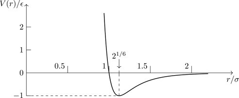
For our purposes, the precise nature of the interactions underlying the potential energy function v(r) is not important as long as there is a long-range attractive component together with a short-range repulsive force. To be definite, we mention the Lennard-Jones potential (shown in Fig. 6.1) for the interaction between closed-shell atoms, which has the parameterized form,
v(r)=4ϵσr12−σr6,
(6.2)
Figure 6.1The Lennard-Jones inter-atomic potential as a function of r/σ.
where ϵ is the depth of the potential well, and σ is the distance at which the potential is zero. The r−6 term describes an attractive interaction between neutral molecules that arises from the energy of interaction between fluctuating multipoles of the molecular charge distributions.3 The r−12 term models the repulsive force at short distances that arises from the Pauli exclusion effect of overlapping electronic orbitals. There’s no science behind the r−12 form; it’s analytically convenient, and it provides a good approximation of the interactions between atoms. For the noble gases, ϵ ranges from 0.003 eV for Ne to 0.02 eV for Xe [18, p398]. The parameter σ is approximately 0.3 nm.
To embark on the statistical-mechanical-road, we have in the canonical ensemble4
where λT occurs from integrating the momentum variables and Q is the configuration integral, the part of the partition function associated with the potential energy of particles,
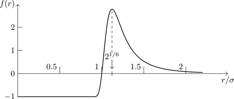
is the Mayer function,5 shown in Fig. 6.2. In the absence of interactions, fij=0, Q=VN, and we recover Eq. (5.1). With interactions, f(r) is bounded between −1 and e−βVmin−1, where Vmin is the minimum value of the interaction potential; f(r) is small for inter-particle separations in excess of the effective range of the potential. Mayer functions allow us to circumvent problems associated with potential functions that diverge6 as r→0. At sufficiently high temperatures, |f(r)|≪1, which provides a way of approximately treating the non-ideal gas.
Figure 6.2Mayer function f(r) associated with the Lennard-Jones potential. βϵ=1.33.
By expanding out the product in Eq. (6.4), a 3N-fold integration is converted into a sum of lower-dimensional integrals known as cluster integrals. The product expands into a sum of terms each involving products of Mayer functions, from zero to all N2=N(N−1)/2 Mayer functions,
where pairs, triples, quadruples, etc., refer to configurations of two, three, four, and so on, particles known as clusters.7 The primes on the summation signs indicate restrictions so that we never encounter terms such as fmm (particles don’t interact with themselves) or f12f12; interactions are between distinct pairs of particles, counted only once. For N=3 particles, Eq. (6.6) generates 232=23=8 terms:
As N increases, the number of terms rises rapidly. For N=4, there are 242=26=64 terms generated by the product; 64 integrals that contribute to Eq. (6.4). Fortunately, many of them are the same; our task is to learn how to characterize and count the different types of integrals. For N=5, there are 1024 terms—we better figure out how to systematically count the relevant contributions to the partition function if we have any hope of treating macroscopic values of N.
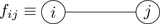
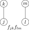
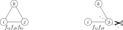
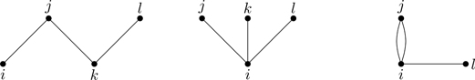
A productive strategy is to draw a picture, or diagram, representing each term in Eq. (6.6). Figure 6.3 shows two circles with letters in them denoting particles at positions ri and rj. The circles represent particles, and the line between them represents the Mayer function fij. Note that the physical distance between i and j is taken into account through the value of the Mayer function; the line in Fig. 6.3 indicates an interaction between particles, regardless of the distance between them. If one were to imagine a numbered circle for each of the N particles of the system, with a line drawn between circles i and j for every occurrence of fij in the terms of Eq. (6.6), every term would be represented by a diagram.8 Let the drawing of diagrams begin!
Figure 6.3Cluster diagram representing the Mayer function fij between particles i,j.
We’ll do that in short order, but let’s first consider what we do with diagrams, a process known as “calculating the diagram.” Starting with two-particle diagrams (Fig. 6.3), for each term associated with ∑pairs′fij in Eq. (6.6), there is a corresponding contribution to Eq. (6.4):
∫dNrfij=VN−2∫dridrjf(|ri−rj|)≡VN−22b2(T)V.
(6.7)
The integrations in Eq. (6.7) over the spatial coordinates not associated with particles i and j leave us with VN−2 on the right side. The cluster integral b2(T) is, by definition,
b2(T)≡12V∫dridrjf(rij)=12∫drf(r)=12∫0∞4πr2f(r)dr.
(6.8)
The second equality in Eq. (6.8) is a step we’ll take frequently. Define a new coordinate system centered at the position specified by ri. With rj−ri≡rji as a new integration variable, we’re free to integrate over ri. We’ll denote this step as dridrj→dridrji. The quantity b2 probes the effective range of the two-body interaction at a given temperature (the second moment of the Mayer function) and has the dimension of (length)3. The cluster expansion method works best when the volume per particle V/N≡1/n is large relative to the volume of interaction, i.e., when nb2≪1. The identity of particles is lost in Eq. (6.8). Thus, the N2=N(N−1)/2 terms in ∑pairs′fij all contribute the same value to the configuration integral. Through first order in Eq. (6.6), we have
Q(N,T,V)=VN1+N(N−1)b2(T)V+⋯.
The partition function (number of states available to the system) is modified (relative to noninteracting particles) by pairs of particles that bring with them an effective volume of interaction, 2b2.
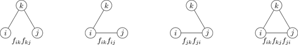
The next term in Eq. (6.6), a sum over three-particle clusters, involves products of two and three Mayer functions. Figure 6.4 shows the diagrams associated with three distinct particles (ijk) joined by two or three lines. For their contribution to Q(T,V,N),
The third line of Eq. (6.10) follows because rik=rij−rkj (and thus the integral is completely determined by rij and rkj; see Exercise 6.2), and we’ve used Eq. (6.8) in the final line. The factor of 3! is included in the definition to take into account permutations of i, j, k, and thus b3is independent of how we label the vertices of the diagram.9 The factor of 3 inside the square brackets comes from the equivalence of the three diagrams in Fig. 6.4 under cyclic permutation, i→j→k→i. The quantity b3 has the dimension of (volume)2.
With Eq. (6.10), we’ve evaluated (formally) the contribution to Q(N,T,V) of a given set of three particles (ijk) that are coupled through pairwise interactions. How many ways can we choose triples? Clearly, N3=N(N−1)(N−2)/3!. Through second order in Eq. (6.6), we have for the configuration integral
Q(T,V,N)=VN1+N(N−1)b2(T)V+N(N−1)(N−2)b3(T)V2+⋯.
6.1.1 Disconnected diagrams and the linked-cluster theorem
It might seem we’ve discerned the pattern now and we could start generalizing. With the next term in Eq. (6.6) (“quadruples”), we encounter a qualitatively new type of diagram. Figure 6.5 shows the diagram associated with the product of two Mayer functions with four distinct indices. The contribution of this diagram to the configuration integral is
Figure 6.5Diagram involving four distinct particles interacting through two pairwise interactions.
where we’ve used Eq. (6.8). What is the multiplicity of this diagram? There are N2×N−22×12=18N(N−1)(N−2)(N−3) distinct ways the cluster in Fig. 6.5 can be synthesized out of N particles. Figure 6.6 shows the three equivalent diagrams for N=4 particles coupled through two pairwise interactions. Including the cluster integral Eq. (6.11) together with its multiplicity,
Figure 6.6Disconnected diagrams of four particles and two pairwise interactions.
It’s not apparent yet, but the term we just added to Eq. (6.12) is bad news.
Let’s think about what we’re trying to do. We seek the partition function for a system of interacting particles. But what do we do with that once we find it? All thermodynamic information can be obtained from the free energy, lnZ (Eq. (4.58) or (4.78)). Write Eq. (6.3), Z(N,T,V)=ZtrQ(N,T,V)/VN, where Ztr is the partition function for the translational degrees of freedom, Eq. (5.1). Then, lnZ=lnZtr+lnQ/VN≡lnZtr+ln1+A, where
A≡[1VN∫dNr∏j>i1+fij]−1.
Make the assumption (to be verified) that A is small compared with unity. Using Eq. (6.12), we can write A=A1+A2+A3+⋯. Apply the Taylor series,10
where we’ve used Eq. (6.10). We know that the free energy is extensive in the thermodynamic limit (see Eq. (4.89)),
limn=N/VfixedN,V→∞N−1F(N,V,T)=f(n,T),
and thus we expect that ln(1+A)~Nf(n,T) as N→∞. Examine Eq. (6.13) for N≫1:
ln(1+A)=N(nb2+2n2b22+12Nn2b22︸Diverges with NTrouble:−12Nn2b22︸Divergent term removedTragedy averted:+⋯).
(6.14)
The first two terms in Eq. (6.14) are indeed intensive quantities that depend on n and T. The third term, however, which comes from the diagram in Fig. 6.5, is not intensive—it scales with N. That’s the bad news in Eq. (6.12)—there are “too many” disconnected diagrams; their contributions prevent the free energy from possessing a thermodynamic limit. Fortunately, the third term in Eq. (6.14) (that scales with N) is cancelled by the fourth term, i.e., A3 (from the disconnected diagram) is cancelled by a term in the Taylor series for ln(1+A), 12A12. Is that a coincidence? Do cancellations like that occur at every order? Formulating an answer is problematic—we’ve relied on a Taylor series that’s valid only when the terms in A are small, yet they’re not small (they scale with N), but at the same time they seem to miraculously disappear from the expansion. Something deeper is at work.
The linked-cluster theorem is a fundamental theorem in graph theory, that only connected diagrams contribute to the free energy. Before stating the theorem (which we won’t prove), let’s try to “psyche out” what the issue is with disconnected diagrams. The diagrams in Fig. 6.4 are linked clusters, where each vertex of a diagram is connected to at least one line. The diagram in Fig. 6.5 is a disconnected cluster—there is not a path between any vertices of the graph. Figure 6.7 shows graphs involving N=3,4,5,6 particles interacting by three lines, where we’ve left the vertices unlabeled (free graphs). The first three are linked clusters, the remaining two are disconnected. Suppose one of the particles, k, in the linked clusters of Fig. 6.4 is far removed from particles i and j; in that case, the Mayer function fik or fjk vanishes, implying that the contribution of the diagram to the configuration integral vanishes. When particles are within an interaction distance, there is a distinct type of energy configuration that’s counted in the partition function. As the particles become sufficiently separated, leaving no interaction among them, such contributions vanish. Now consider the disconnected diagrams, such as in Fig. 6.5 or 6.7: One can freely separate the disjoint parts of the diagram (which are not in interaction with each other), placing them anywhere in the system, in which case the interactions represented by the disconnected parts have already been counted in the partition function. The expansion we started with in Eq. (6.6) generates disconnected diagrams, which overcount various configurations. The linked-cluster theorem tells us that only connected diagrams contribute to the free energy (and thus to all thermodynamic information). We need evaluate the partition function taking into account connected diagrams only.
Figure 6.7Diagrams composed of three lines. The first three are linked, the last two are not.
The precise form of the linked-cluster theorem depends on whether we’re in the classical or quantum realm, Fermi or Bose, but the central idea remains the same. We present a version given by Uhlenbeck and Ford[55, p40]. Consider a quantity FN that’s a weighted sum over the graphs GN (connected or disconnected) of N labeled points, FN≡∑GNW(GN), where W(GN), the weight given to a graph, is in our application the product of the multiplicity and the cluster integral associated with that type of graph. The N-particle configuration integral Q(N,T,V) is just such a function as FN. Define another quantity fl as a weighted sum over connected graphs, fl≡∑ClW(Cl), where the sum is over the connected graphs Cl (of the set GN) with labeled points. The theorem states that
1+F(x)=ef(x),
(6.15)
where F(x) and f(x) are generating functions11 of the quantities FN and fl:
F(x)≡∑N=1∞FNxNN!f(x)≡∑l=1∞flxll!.
(6.16)
So far, we’ve considered the case of fixed N, yet the generating functions in Eq. (6.15) apply for an unlimited number of particles. That finds a perfect application in the grand canonical ensemble, which is where we’re heading (see Section 6.1.3). The linked-cluster theorem can be remembered as the equality
∑all diagrams=exp∑(all connected diagrams).
6.1.2 Obtaining Z(N,T,V)
We now give a general definition of the cluster integral associated with n-particle diagrams:
bn(T)≡1n!V∑n-particle diagramsall connected∫(∏connected n-particle diagramlk∈the set of bonds in aflk)dr1⋯drn.
(6.17)
Equation (6.17) is consistent with Eqs. (6.8) and (6.10) for n=2,3. (By definition, b1=1.) The purpose of the factor of n! is to make the value of bn independent of how we’ve labeled the n vertices of the diagram (required by the linked-cluster theorem), and the factor of 1/V cancels the factor of V that always occurs in evaluating cluster integrals of connected diagrams—we’re free to take one vertex of the graph and place it anywhere in the volume V. The quantity bn has the dimension of (volume)n−1: For an n-particle diagram, we integrate over the coordinates of n−1 particles relative to the position of the nth particle. The cluster integral bn is therefore independent of the volume of the system as long as V is not too small.
There are many ways that a given set of particles can be associated with clusters. Suppose K particles are partitioned into m2 two-particle clusters, m3 three-particle clusters, and so on. The integral over dr1⋯drN of this collection of clusters factorizes (because each cluster is connected)
(1!Vb1)m1(2!Vb2)m2⋯(j!Vbj)mj⋯=∏j=1N(j!Vbj)mj,
(6.18)
where, to systematize certain formulas we’re going to derive, we’ve introduced the unit cluster, b1, which is not a particle; such terms contribute the factors of VN−K seen in Eqs. (6.7) and (6.9). Associated with any given placement of N particles into a cluster is a constraint,
∑l=1Nlml=N.
(6.19)
Figure 6.8 shows a set of diagrams for N=4 particles in which we show the unit clusters. You should verify that Eq. (6.19) holds for each of the diagrams in Fig. 6.8.
Figure 6.8Some of the diagrams for a system of N=4 particles, including the unit clusters. In the first m2=1 and m1=2, in the second m3=1 and m1=1, and in the third, m4=1 and m1=0.
How many distinct ways can N distinguishable particles12 be partitioned into m1 unit clusters, m2 two-particle clusters, ⋯, mj clusters of j-particles, and so on? The number of ways of dividing N distinguishable objects among labeled boxes so that there is one object in each of m1 boxes, two objects in each of m2 boxes, etc., is given by the multinomial coefficient, Eq. (3.12),
N!(1!)m1(2!)m2⋯(j!)mj⋯.
We don’t want to count as separate, however, configurations that differ by permutations among clusters of the same kind. To prevent overcounting, we have to divide the multinomial coefficient by m1!m2!⋯mj!⋯. The combinatorial factor is therefore
N!∏j=1N(j!)mjmj!.
(6.20)
The contribution to the configuration integral of the collection of clusters characterized by the particular set of integers {mj} is therefore the product of the expressions in (6.18) and (6.20):
N!∏jj!Vbjmj(j!)mjmj!=N!∏jVbjmjmj!.
(6.21)
Note that we don’t need to indicate the range of the index j—clusters for which mj=0 don’t affect the value of the product.
There will be a contribution to the configuration integral for each set of the numbers {mj},
Q(N,T,V)=N!∑{mj}∑j=1Njmj=N∏j=1N(Vbj)mjmj!,
(6.22)
where ∑{mj} indicates to sum over all conceivable sets of the numbers mj that are consistent with Eq. (6.19). For the noninteracting system, there are no clusters: m1=N with mj≠1=0, for which Eq. (6.22) reduces to VN. The partition function for N particles is therefore (see Eq. (6.3)):
Z(N,T,V)=1λT3N∑{mj}∑j=1Njmj=N∏j=1N(Vbj)mjmj!.
(6.23)
6.1.3 Grand canonical ensemble, ZG(μ,T,V)
Equation (6.23) is similar to Eq. (5.49) (the partition function of ideal quantum gases). For quantum systems, we have sums over occupation numbers, which satisfy a constraint, ∑k,σnk,σ=N. Here we have a constrained sum over mj, the number of j-particle clusters.13 And just as with Eq. (5.49), Eq. (6.23) is impossible to evaluate because of the combinatorial problem of finding all sets of numbers {mj} that satisfy ∑jjmj=N. But, just as with Eq. (5.49), Eq. (6.23) simplifies in the grand canonical ensemble, where the constraint of a fixed number of particles is removed.
Combining Eq. (6.23) with Eq. (4.77) (where z=eβμ is the fugacity), we have the grand partition function (generating function for the quantities {ZN})
where the transition to the second line of Eq. (6.24) follows from the same reasoning used in the transition from Eq. (5.50) to Eq. (5.51), ξ≡eβμ/λT3, and we’ve used Eq. (6.19) for N. We can then sum the infinite series14 in Eq. (6.24), with the result
ZG(μ,T,V)=∏j=1∞expVbjξj=exp(V∑j=1∞bjξj).
(6.25)
Equation (6.25) reduces to Eq. (4.79) in the noninteracting case. From ZG, we have the grand potential (see Eq. (4.76))
Φ(T,V,μ)=−kTlnZG(T,V,μ)=−kTV∑j=1∞bjξj.
(6.26)
The thermodynamics of interacting gases is therefore reduced to evaluating the cluster integrals bj.
These formulas are fugacity expansions ( ξ=z/λT3), such as we found for the ideal quantum gases (Section 5.5.3). It’s preferable to express P in the form of a density expansion (density is more easily measured than chemical potential). We can invert the expansion for N to obtain a density expansion of the fugacity. Starting from n=∑j=1∞jbjξj in Eq. (6.27), we find using standard series inversion methods, through third order in n:
eβμλT3=ξ=n−2b2n2+8b22−3b3n3+O(n4).
(6.28)
Equation (6.28) should be compared with Eq. (5.71). Substituting Eq. (6.28) into the expression for P in Eq. (6.27), we find, through second order,
P=nkT1−b2n+4b22−2b3n2+O(n3).
(6.29)
Equation (6.29), a density expansion of P, is known as the virial expansion. It reduces to the ideal gas equation of state in the case of no interactions.
The virial expansion was introduced (in 190116) as a parameterized equation of state,
P=nkT1+B2(T)n+B3(T)n2+B4(T)n3+⋯,
where the quantities Bn(T) are the virial coefficients, which are tabulated for many gases.17 Virial coefficients are not measured directly; they’re determined from an analysis of PVT data. The most common practice is a least-squares fit of PV values along isotherms as a function of density. Statistical mechanics provides (from Eq. (6.29)) theoretical expressions for the virial coefficients:
B2=−b2B3=4b22−2b3B4=−20b23+18b2b3−3b4,
(6.30)
where the expression for B4 is the result of Exercise 6.6. The virial coefficients require inter-particle interactions for their existence. For example, using Eq. (6.8),
B2(T)=−12∫drf(r).
(6.31)
An equation of state proposed by van der Waals18 in 1873 takes into account the finite size of atoms as well as their interactions. The volume available to gas atoms is reduced (from the volume V of the container) by the volume occupied by atoms. Van der Waals modified the ideal gas law, to
P=NkTV−Nb,
where b>0 is an experimentally determined parameter for each type of gas. The greater the number of atoms, the greater is the excluded volume. Van der Waals further reasoned that the pressure would be lowered by attractive interactions between atoms. The decrease in pressure is proportional to the probability that two atoms interact, which, in turn, is proportional to the square of the particle density. In this way, van der Waals proposed the equation of state,
P=NkTV−Nb−an2,
where a>0 is another material-specific parameter to be determined from experiment.19 The van der Waals equation of state is usually written
P+an2(V−Nb)=NkT.
(6.32)
It’s straightforward to show that Eq. (6.32) implies for the second virial coefficient,
B2vdw(T)=b−akT.
(6.33)
The van der Waals equation of state provides a fairly successful model of the thermodynamic properties of gases. It doesn’t predict all properties of gases, but it predicts enough of them for us to take the model seriously. It’s the simplest model of an interacting gas we have. Can the phenomenological parameters of the model, (a,b), can be related to the properties of the inter-particle potential? Let’s see if the second virial coefficient as predicted by statistical mechanics, −b2, has the form of that in Eq. (6.33), i.e., can we establish the correspondence
b2↔?−b+akT
for suitably defined quantities (a,b) ? To do that, let’s calculate b2 for the Lennard-Jones potential. From Eq. (6.8),
12πb2=∫0∞r2e−βv(r)−1dr≈−∫0σr2dr−β∫σ∞v(r)r2dr,
(6.34)
where, referring to Fig. 6.2, for 0≤r≤σ we’ve taken the repulsive part of the potential as infinite (hard core potential) so that the Mayer function is equal to −1, and for r≥σ we’ve approximated the Mayer function with its high-temperature form, −βv(r). With these approximations, we find
b2=−2π3σ3+16π9ϵkTσ3.
(6.35)
The correspondence therefore holds: b~σ3 is an excluded volume provided by the short-range repulsive part of the inter-particle potential, and the parameter a~ϵσ3 is an energy-volume associated with the attractive part of the potential. Statistical mechanics validates the assumptions underlying the van der Waals model, illustrating the role of microscopic theories in deriving phenomenological theories. Moreover, as we now show, with some more analysis we can provide a physical interpretation of the types of interactions that give rise to the virial coefficients.
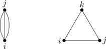
We now derive the virial expansion in another way, one that features additional techniques of diagrammatic analyses.20 Consider B3=2(2b22−b3); Eq. (6.30). Using Eq. (6.10) (for b3), we see that a cancellation occurs among the terms contributing to B3, leaving us with one integral:
B3=−13∫drijdrkjf(rik)f(rkj)f(rij).
(6.36)
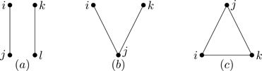
The diagram corresponding to this integral is shown in the left part of Fig. 6.9. What about the diagrams that don’t contribute to B3? Time for another property of diagrams. A graph is irreducible when each vertex is connected by a bond to at least two other vertices, as in the left part of Fig. 6.9.21 A reducible graph has certain points, articulation points, where it can be cut into two or more disconnected parts, as in the right part of Fig. 6.9. Graphs can have more than one articulation point; see Fig. 6.10. A linked graph having no articulation points is irreducible. Figure 6.11 shows the three types of diagrams: Unlinked, reducible, and irreducible. As we now show, only irreducible diagrams contribute to the virial coefficients.
Figure 6.9Irreducible (left) and reducible (right) connected clusters of three particles.
Figure 6.10Example of a graph with two articulation points (open circles)
Figure 6.11Three types of graphs: (a) Unlinked (not all vertices connected by bonds); (b) reducibly linked (every vertex connected by a least one bond); (c) irreducibly linked (every vertex connected by at least two bonds).
Rewrite Eq. (6.3) (as we did in Section 6.1.1), Z(T,V,N)=ZtrQ(T,V,N)/VN, where Ztr is the partition function for the ideal gas, Eq. (5.1). We now write Q/VN in a new way:
where V(r1,⋯,rN)≡∑j>iv(rij) is the total potential energy of particles having the instantaneous positions r1,⋯,rN, and we’ve introduced a new average symbol,
〈(⋯)〉0≡1VN∫dNr(⋯).
Equation (6.37) interprets the configuration integral as the expectation value of e−βV(r1,⋯,rN) with respect to a non-thermal (in fact, geometric) probability distribution22 where the variables r1,⋯,rN have a uniform probability density (1/V)N inside a container of volume V. Using Eq. (4.57), we obtain
−βF−Fideal=ln〈e−βV(r1,⋯,rN)〉0,
(6.38)
where Fideal≡−kTlnZtr is the free energy of the ideal gas. The right side of Eq. (6.38) is the contribution to the free energy arising solely from inter-particle interactions.
We encountered just such a quantity in Eq. (3.34), the moment generating function 〈eθx〉=∑n=0∞θn〈xn〉/n!, where, we stress, the average symbols 〈〉 are associated with a given (not necessarily thermal) probability distribution. The logarithm of 〈eθx〉 defines the cumulant generating function, Eq. (3.59),23
ln〈eθx〉=∑n=1∞θnn!Cn,
(6.39)
where each quantity Cn (cumulant) contains combinations24 of the moments 〈xk〉, 1≤k≤n. Explicit expressions for the first few cumulants are listed in Eq. (3.62). To apply Eq. (6.39) to Eq. (6.38), set θ=−β and associate the random variable x with the total potential energy, V=∑j>iv(rij). Thus we have the cumulant expansion of the free energy (with ΔF≡F−Fideal):
where we’ve used Eq. (3.66), that the cumulant associated with a sum of independent random variables is the sum of cumulants associated with each variable. We’re interested in the thermodynamic limit. Making use of Eq. (3.44), Nn~N→∞Nn/n!, in Eq. (6.41),
limN/V=nN,V→∞C1N=12n∫v(r)dr.
(6.42)
Cumulants must be extensive, so that the free energy as calculated with Eq. (6.40) is extensive.25 We associate the integral in Eq. (6.42) with the graph in Fig. 6.12, which is nominally the same as Fig. 6.3, with an important exception—Fig. 6.3 represents the Mayer function fij between particles i,j, whereas Fig. 6.12 represents their direct interaction, vij.
Figure 6.12The one diagram contributing to C1.
The cumulant C2 is the fluctuation in potential energy:26
where vij≡v(rij). Let’s analyze the structure of the indices in Eq. (6.43), because that’s the key to this method. There are three and only three possibilities in this case:
No indices in common; unlinked terms. Consider 〈v12v34〉0. Because we’re averaging with respect to a probability distribution in which r12 and r34 can be varied independently,
〈v12v34〉0=〈v12〉0〈v34〉0.
(6.44)
The averages of products of potential functions with distinct indices factor, and as a result C2 vanishes identically—a fortunate development: There are 12N2N−22~N→∞N4/8 ways to choose, out of N indices, two sets of pairs having no elements in common. We’ll call terms that scale with N too rapidly to let the free energy have a thermodynamic limit, super extensive. The important point is that every unlinked term arising from 〈vijvkl〉0 (which we’re calling super extensive) is cancelled by a counterpart, 〈vij〉0〈vkl〉0. The diagrams representing 〈vijvkl〉0 for no indices in common are those in Fig. 6.11(a).
One index in common; reducibly-linked terms. Consider 〈v12v23〉0:
Because of the averaging procedure 〈〉0, 〈v12v23〉0 factorizes, implying that C2 vanishes for these terms. Such terms correspond to reducibly linked diagrams (see Fig. 6.11(b))—the common index represents an articulation point where the graph can be cut and separated into disconnected parts. Reducible graphs make no contribution to the free energy.
Both pairs of indices in common; irreducibly-linked graphs. Consider the case, from Eq. (6.43), where k=i and l=j,
C2=∑j>i〈vij2〉0−〈vij〉02.
(6.46)
The first term in Eq. (6.46), the average of the square of the inter-particle potential,
〈vij2〉0=1V2∫dridrjvij2→1V∫drijvij2≡1V∫drv2(r)~1V,
(6.47)
whereas
〈vij〉02=1V∫drv(r)2~1V2.
(6.48)
We’re assuming the integrals ∫drv(r) and ∫drv2(r) exist. Noting how the terms scale with volume in Eqs. (6.47), (6.48), only the first term survives the thermodynamic limit,
limN/V=nN,V→∞C2N=12n∫v2(r)dr,
(6.49)
where we’ve used ∑j>i=N2. Figure 6.13 shows the diagram representing the integral in Eq. (6.49). This is a new kind of diagram where vij2 is represented by two bonds between particles i,j; it has no counterpart in the Mayer cluster expansion (we never see terms like f12f12).
Figure 6.13The one diagram contributing to C2.
Most of the complexity associated with higher-order cumulants is already present in C3, so let’s examine it in detail.
For all indices distinct, i≠j≠k≠l≠m≠n, the average of three potential functions factors,
〈vijvklvmn〉0=〈vijvkl〉0〈vmn〉0=〈vij〉0〈vkl〉0〈vmn〉0,
and C3=0. Disconnected diagrams (Fig. 6.14(a)) make no contribution. There are other kinds of unlinked diagrams, however. For one index in common between a pair of potential functions ( l=j, for example), with no overlap of indices from the third function, we have (see Fig. 6.14(b))
〈vijvjkvmn〉0=〈vijvjk〉0〈vmn〉0,(m,n≠i,j,k)
and C3 vanishes. If we set k=i (with l=j and m,n≠i,j), C3=0 for the diagram in Fig. 6.14(c). All unlinked diagrams arising from〈vijvklvmn〉0are cancelled by the terms ofC3.
Figure 6.14The unlinked diagrams associated with 〈vijvklvmn〉0: (a) i≠j≠k≠l≠m≠n; (b) l=j and m,n≠i,j,k; (c) l=j and k=i, m,n≠i,j. C3=0 for these diagrams.
The reducible diagrams associated with 〈vijvklvmn〉0 (see Fig. 6.15) make no contribution to C3. For the left diagram in Fig. 6.15, 〈vijvjkvkl〉0 factors into 〈vij〉0〈vjk〉0〈vkl〉0 on passing to relative coordinates. For the middle diagram, 〈vijvikvil〉0=〈vij〉0〈vik〉0〈vil〉0, and for that on the right, 〈vij2vil〉0=〈vij2〉0〈vil〉0. In all cases, C3=0 for reducible diagrams.
Figure 6.15The reducible diagrams associated with 〈vijvklvmn〉0. C3=0 for these diagrams.
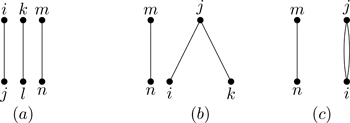
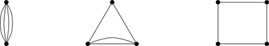
That leaves the irreducible diagrams, for which C3≠0. The two (and only two) irreducible diagrams associated with 〈vijvklvmn〉0 are shown in Fig. 6.16. There are N2 contributions of the diagram on the left, and N(N−1)(N−2) contributions of the diagram on the right. In the thermodynamics limit,
Figure 6.16The two (irreducible) diagrams having nonzero contributions to C3.
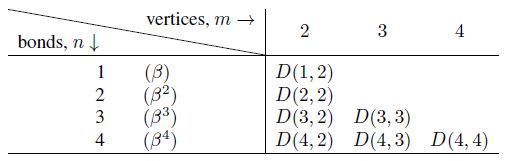
These examples show that only irreducible diagrams contribute to the cumulant expansion of the free energy. Unlinked and reducible parts of cumulants either cancel identically, or don’t survive the thermodynamic limit. Whatever are the unlinked or reducible graphs in a cumulant, factorizations occur such as in Eq. (6.45), causing it to vanish. The nonzero contributions to Cn consist of the irreducible clusters arising from the leading term,27〈Vn〉0. Our task therefore reduces to finding all irreducible diagrams at each order. Figure 6.17 shows the three (and only three) irreducible diagrams at order n=4. The graphs associated with 〈Vn〉0 have n bonds because each of the n copies of the potential function vij represents a bond. Such graphs have m vertices, 2≤m≤n. One can have n powers of a single term vij, in which case m=2, up to the case of m=n vertices which occurs for a diagram like 〈v12v23v34v41〉0 (a cycle in graph-theoretic terms). Let D(n,m) denote an irreducible diagram having n bonds and m vertices. Table 6.1 lists the irreducible diagrams classified by the number of bonds n ( n≤4) and the number of vertices, 2≤m≤n. The diagram D(1,2) is shown in Fig. 6.12, D(2,2) is shown in Fig. 6.13, D(3,2) and D(3,3) are shown in Fig. 6.16, and D(4,2), D(4,3), and D(4,4) are shown in Fig. 6.17. Each cumulant Cn>1 can be written, in the thermodynamic limit, as a sum of irreducible diagrams, Cn=∑m=2nD(n,m). The case of C1 is special: C1=D(1,2).
Figure 6.17Irreducible diagrams associated with n=4 bonds and m=2,3,4 vertices.
Table 6.1Irreducible graphs D(n,m) classified by number of bonds n and vertices 2≤m≤n.
Thus, the free energy is determined by irreducible diagrams, but we haven’t shown (as advertised) that the virial coeficients are so determined. Returning to Eq. (6.40), we can write
−βΔF=∑n=1∞(−β)nn!Cn=∑n=1∞(−β)nn!∑m=2nD(n,m),
where we’ve in essence summed “across” the entries in Table 6.1 for each n (which is natural—that’s how the equation is written). We can reverse the order of summation, however, and sum over columns,
where we’ve used Eq. (6.8). Thus, the sum over the class of irreducible diagrams D(n,2) has reproduced (up to multiplicative factors) the cluster integral b2. It can then be shown from (6.52) that (see Exercise 6.12)
P=nkT1+B2n+⋯,
(6.53)
where B2=−b2, Eq. (6.30). We’ll stop now, but the process works the same way for the other virial coefficients—summing over irreducibly linked, topologically distinct diagrams associated with the same number of vertices, one arrives at irreducible cluster integrals for each virial coefficient, such as we’ve seen already for B2 and B3, Eqs. (6.31) and (6.36).
Consider a system of N identical particles confined to a one-dimensional region 0≤x≤L that interact through an inter-particle potential energy function ϕ(x). In the Tonks gas[59], ϕ(x) has the form
ϕ(x)=∞|x|<a0|x|>a,
(6.54)
which is therefore a collection of hard rods of length a. The Takahashi gas29 is a generalization with
ϕ(x)=∞|x|<av(x−a)a<|x|<2a0|x|>2a,
(6.55)
which is a collection of hard rods with nearest-neighbor interactions.30
Note the factor of hN and not h3N —we’re in one spatial dimension with N particles. The integrand is a totally symmetric function of its arguments (x1,⋯,xN), which can be permuted in N! ways. One can show31 for f(x1,⋯,xN) a symmetric function, the multiple integral ∫0L⋯∫0Lfdx1⋯dxN over an N-dimensional cube of length L is equal to N! times the nested integrals: N!∫0LdxN∫0xNdxN−1⋯∫0x2fdx1. This ordering of the integration variables such that 0≤x1⋯≤xN≤L allows us to evaluate the configuration integral exactly.
For the Tonks gas, which has only the feature of a hard core, the Boltzmann factors are either zero or one:
exp(−β∑1≤i≤j≤Nϕ(|xi−xj|))=∏1≤i≤j≤NS(|xi−xj|),
(6.57)
where
S(x)≡1|x|>a0|x|<a.
The region of integration for the configuration integral is therefore specified by |xi−xj|>a for all i,j. It should be noted that in the sum ∑j>iϕ(|xi−xj|), every particle in principle interacts with every other particle, even though in this example the interactions between particles are zero except when they’re close enough to encounter the hard core of the potential. Given the aforementioned result on symmetric functions, we can set j=i+1 in Eq. (6.57), with the region of integration specified by the inequalities xi+1>xi+a, i=1,⋯,N−1. Referring to Fig. 6.18, we see that 0≤x1<x2−a, a<x2<x3−a, ⋯, (i−1)a<xi<xi+1−a, ⋯, (N−1)a<xN≤L. With a change of variables, yi=xi−(i−1)a, i=1,⋯,N,
Figure 6.18Region of integration for the partition function of a one-dimensional gas of hard rods.
where l≡L−(N−1)a is the free length available to the collection of rods; (N−1)a is the excluded volume (length). We see the “return” of the factor of N!.
With Z(L,N,T) in hand, we can calculate the free energy and the associated thermodynamic quantities μ,P,S (see Eq. (4.58)). Starting from Eq. (4.57), and using Eq. (6.58),
where we’ve used Stirling’s approximation for N≫1. The pressure is obtained from
P≡−∂F∂LN,T=NkTL−Na.
(6.60)
Pressure in one dimension is an energy per length—an energy density—just as pressure in three dimensions is an energy density, energy per volume, or force per area. One-dimensional pressure is simply a force—an effective force experienced by hard rods. We see the excluded volume effect in Eq. (6.60), just as in the van der Waals equation of state; there is clearly no counterpart to the other parameter of the van der Waals model. The entropy and chemical potential are found from the appropriate derivatives of the free energy, with the results:
S=Nk32+lnL−NaNλT;
(6.61)
βμ=NaL−Na−lnL−NaNλT.
(6.62)
Equation (6.61) becomes, in the limit a→0, the formula for the entropy of a one-dimensional ideal gas (see Exercise 5.2). We see from Eq. (6.62) a positive contribution to the chemical potential from the repulsive effect of the hard core potential (for L>Na).
In the thermodynamic limit ( N→∞, L→∞, v≡L/N fixed), these quantities reduce to the expressions (from Eqs. (6.59)–(6.62)),
The thermodynamic limit therefore exists (something already known from Section 4.2): Extensive quantities (F,S) are extensive, and intensive quantities ( P,μ) are intensive. The free energy (from which the other quantities are found by taking derivatives) is an analytic function of v for v>a, where v=L/N is the average length per particle. For v<a, rods overlap, which from Eq. (6.56) implies that Z(L,N,T)=0 when N/L>a−1, where a−1 is the close packing density.
The thermodynamic quantities associated with this one-dimensional system become singular at the close-packing point, v=a. What is the significance, if any, of the occurrence of such singularities and the vanishing of the partition function? We expect the vanishing of the partition function as a generic feature of systems featuring purely hard core potentials. Consider, in any dimension d, the canonical partition function
Z(V,N,T)=1λTdN1N!∫dNr∏1≤i≤j≤NS(|ri−rj|),
(6.64)
where the quantities ri are d-dimensional vectors, and we’ve used Eq. (6.57). The partition function vanishes for densities exceeding the close packing density n0≡Nmax/V, where Nmax is the maximum number of hard spheres of radius a that can be contained in the volume V. It might be thought that the vanishing of Z at the close packing density signals a phase transition from a gaseous to a solid phase.32 It was conjectured in 1939 that a system of particles with hard-core potentials would undergo a phase transition at a density well below the close packing density[63]; evidence was first found in computer simulations[64]. A phase transition associated with purely repulsive interactions is known as the Kirkwood-Alder transition. Evidence for this transition has been found experimentally in colloidal suspensions [65].
For the Takahashi gas, we have, instead of Eq. (6.58),
Equation (6.65) is in the form of an iterated Laplace convolution, which suggests a method of solution. Take the Laplace transform of Z as a function of l. It can be shown from Eq. (6.65) that
Z˜(s)≡∫0∞e−lsZ(L,N,T)dl=1λTN1s2K(s)N−1,
(6.66)
where
K(s)≡∫0∞e−sx−βv(x)dx.
(6.67)
The partition function then follows by finding the inverse Laplace transform of Z˜(s). Without specifying the form of the potential function v(x), this is about as far as we can go. The method cannot be extended to systems having more than nearest-neighbor interactions. Thus, the partition function of a one-dimensional collection of particles having hard core potentials can be solved exactly for nearest-neighbor interactions only.
The Ising model, conceived in 1924 as a model of magnetism, has come to occupy a special place in theoretical physics with an enormous literature.33 Consider a one-dimensional crystalline lattice—a set of uniformly spaced points (lattice sites) separated by a distance a. Referring to Fig. 6.19, at each lattice site assign the value of a variable that can take one of two values, conventionally denoted σi=±1, i=1,⋯,N, where N is the number of lattice sites. The variables σi can be visualized as vertical arrows, up or down (as in Fig. 6.19), and for that reason are known as Ising spins. Real spin- 12 particles have two values of the projection of their spin vectors S onto a pre-selected z-axis, Sz=±12ℏ, and thus Sz can be written Sz=12ℏσ, but that is the extent to which Ising spins have any relation to quantum spins. Ising spins are two-valued classical variables. In this section we consider one-dimensional systems of Ising spins, which can be solved exactly. Ising spins on two-dimensional lattices can also be solved exactly, but the mathematics is more difficult. We touch on the two-dimensional Ising model in Chapter 7; what we learn here will help.
Figure 6.19One-dimensional system of Ising spins with lattice constant a.
Paramagnetism was treated in Chapter 5 in which independent magnetic moments interact with an externally applied magnetic field. Many other types of magnetic phenomena occur as a result of interactions between moments located on lattice sites of crystals. In ferromagnets, moments at widely separated sites become aligned, spontaneously producing (at sufficiently low temperatures) a magnetized sample in the absence of an applied field. In antiferromagnets, moments become anti-aligned at different sites, in which there is a spontaneous ordering of the individual moments, even though there is no net magnetization. The Heisenberg spin Hamiltonian models the coupling of spins Si,Sj located at lattice sites (i,j) in the form H=−∑ijJijSi·Sj, where the coefficients Jij are the exchange coupling constants.34 Positive (negative) exchange coefficients promote ferromagnetic (antiferromagnetic) ordering. The microscopic underpinnings of the interaction Jij is a complicated business we won’t venture into.35 In statistical mechanics, the coupling coefficients are taken as given parameters. The symbol Si strictly speaking refers to a quantum-mechanical operator, but in many cases is approximated as a classical vector. The Ising model replaces Si with its z-component, normalized to unit magnitude.
We take as the Hamiltonian for a one-dimensional system of Ising spins having nearest-neighbor interactions,36
H(σ1,⋯,σN)=−J∑i=1N−1σiσi+1−b∑i=1Nσi.
(6.68)
The magnetic field parameter b is an energy (Ising spins are dimensionless) and thus b=μBB¯, where μB is the Bohr magneton and B¯ is the “real” magnetic field. We’re going to reserve B (a traditional symbol for magnetic field) for a dimensionless field strength, B≡βb. We’ll also define a dimensionless coupling constant K≡βJ. It’s obvious, but worth stating: Equation (6.68) specifies the magnetic energy of a given assignment of spin values (σ1,⋯,σN). The recipe of statistical mechanics is to sum over all 2N possible configurations in obtaining the partition function.
6.5.1 Zero external field, free boundaries
The canonical partition function for N Ising spins in one dimension having nearest-neighbor interactions in the absence of an applied magnetic field and for free boundary conditions is obtained from the summation:37
and we’ve used that coshx is an even function. For Ising spins we have the useful identity
eKσ=coshK+σsinhK,
(6.70)
and thus ∑σ=−11eKσ=2coshK. The notational convention ∑{σ} saves writing—it indicates a sum over all 2N spin configurations. The final equality in Eq. (6.69) is a recursion relation which is easily iterated to obtain an expression for the partition function:
ZN(K)=2NcoshN−1(K).
(6.71)
A good check on a formula like Eq. (6.71) is to set K=0 ( T→∞), corresponding to uncoupled spins, for which ZN(K=0)=2N.
From ZN(K), we can find the internal energy and the entropy using Eqs. (4.40) and (4.58):
Figure 6.20 is a plot of S versus T. Entropy is maximized at Nkln2 for high temperatures, kT≳10|J|: there are 2N configurations associated with uncoupled spins. The entropy vanishes at low temperature, kT≪|J| (third law of thermodynamics). Note how the entropy of Ising spins differs from that of the ideal gas. In the ideal gas, entropy is related to the kinetic energy of atoms (the only kind of energy atoms of an ideal gas can have); it diverges logarithmically at high temperatures and is unbounded. For Ising spins there is no contribution from kinetic energy; the energy of interaction is all potential. “Phase space” for Ising spins (configuration space) is finite;39 phase space for the ideal gas (momentum space) is unbounded.
Figure 6.20Entropy of a one-dimensional system of Ising spins versus temperature.
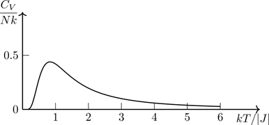
The heat capacity for the one-dimensional Ising model is, from either expression in Eq. (6.72),
CV=∂U∂T=T∂S∂T=k(N−1)K21−tanh2K.
(6.74)
This function is plotted in Fig. 6.21 for N≫1. Note that the maximum in CV occurs at roughly the same temperature at which the slope of S(T) in Fig. 6.20 is maximized. The configuration of the system associated with the maximum rate of change of entropy with temperature (heat capacity) is the configuration at which energy is most readily absorbed.
Figure 6.21Heat capacity of a one-dimensional system of Ising spins versus temperature. Vertical scale the same as in Fig. 6.20.
6.5.2 The transfer matrix method
The method of analysis leading to the recursion relation in Eq. (6.69) does not generalize to finite magnetic fields (try it!). We now present a more general technique for calculating the partition function of spin models, the transfer matrix method, which applies to systems satisfying periodic boundary conditions. Figure 6.22 shows a system of N Ising spins that wraps around on itself40 with σN+1≡σ1. The Hamiltonian
H=−J∑i=1Nσiσi+1−b∑i=1Nσi.(σN+1≡σ1)
(6.75)
Figure 6.22One-dimensional Ising model with periodic boundary conditions, σN+1≡σ1.
The only difference between Eqs. (6.75) and (6.68) is the spin interaction σNσ1.
The partition function requires us to evaluate the sum
ZN(K,B)=∑{σ}expK∑i=1Nσiσi+1+B∑i=1Nσi,
(6.76)
where B=βb. The exponential in Eq. (6.76) can be factored,41 allowing us to write
ZN(K,B)=∑{σ}V(σ1,σ2)V(σ2,σ3)⋯V(σN−1,σN)V(σN,σ1),
(6.77)
where
V(σi,σi+1)≡expKσiσi+1+12B(σi+σi+1)
(6.78)
is symmetric in its arguments,42V(σi,σi+1)=V(σi+1,σi).
Equation (6.77) is in the form of a product of matrices. We can regard V(σ,σ′) as the elements of a 2×2 matrix, V, the transfer matrix,43 which, in the “up-down” basis σj=±1, has the form
V=(+)(−)e(+)K+Be(−)−Ke−KeK−B.
(6.79)
Holding σ1 fixed in Eq. (6.77) and summing over σ2,⋯,σN, Z is related to the trace of an N-fold matrix product,
ZN(K,B)=∑σ1VN(σ1,σ1)=TrVN.
(6.80)
Finding an expression for the Nth power of V, while it can be done (see Exercise 6.24), is unnecessary. The trace is independent of the basis in which a matrix is represented;44 matrices are diagonal in a basis of their eigenfunctions, with their eigenvalues λi occurring as the diagonal elements—so choose that basis. The Nth power of a diagonal matrix D is itself diagonal with elements the Nth power of the elements of D. The transfer matrix Eq. (6.79) has two eigenvalues, λ±. The trace operation in Eq. (6.80) is therefore easily evaluated,45 with
ZN(K,B)=λ+N+λ−N,
(6.81)
where the eigenvalues of V are readily ascertained (show this),
λ±(K,B)=eKcoshB±e−K1+e4Ksinh2B.
(6.82)
Because λ+>λ−,
ZN(K,B)=λ+N1+λ−λ+N~N→∞λ+N.
(6.83)
For large N, ZN and hence all thermodynamic information is contained in the largest eigenvalue, λ+. For B=0, λ+(K,B=0)=2coshK, and ZN(K,0) from Eq. (6.83) agrees with ZN(K) from Eq. (6.71) in the thermodynamic limit.46
The average magnetization M≡〈∑iσi〉=N〈σ〉 can be calculated from ZN(K,B):
〈σ〉=limN→∞1N∂lnZN∂B=e2KsinhB1+e4Ksinh2B.
(6.84)
The system is paramagnetic (even with interactions between spins): As B→0, 〈σ〉→0. The zero-field susceptibility per spin, when calculated from Eq. (6.84), has the value
χ=1N∂M∂B|B=0=e2K.
(6.85)
The susceptibility can be calculated in another way. It’s readily shown for N→∞ that
χ=1N∂M∂B|B=0=1N∑i∑j〈σiσj〉B=0=1+tanhK1−tanhK.
(6.86)
The susceptibility is therefore the sum of all two-spin correlation functions〈σiσj〉, a topic to which we now turn. It’s straightforward to show that Eq. (6.86) is equivalent to Eq. (6.85).
6.5.3 Correlation functions
Correlation functions (such as 〈σiσj〉) play an important role in statistical mechanics and will increasingly occupy our attention in this book; they provide spatial, structural information that cannot be obtained from partition functions.47,48 We can calculate correlation functions of Ising spins using the transfer matrix method, as we now show. Translational invariance (built into periodic boundary conditions, but attained in any event in the thermodynamic limit) implies that 〈σiσj〉 is a function of the separation between sites (i,j), 〈σiσj〉=f(|i−j|). The quantity 〈σiσj〉 is in some sense a conditional probability: Given that the spin at site i has value σi, what is the probability that the spin at site j has value σj? That is, to what extent is the value of σjcorrelated49 with the value of σi? We expect the closer spins are spatially, the more they are correlated. Correlation functions establish a length, the correlation length, ξ, a measure of the range over which correlations persist. We expect for separations far in excess of the correlation length, |i−j|≫ξ, that 〈σiσj〉→〈σ〉2.
Because V(σ1,σ2)⋯V(σN,σ1)/ZN is the probability the system is in state (σ1,⋯,σN) (for periodic boundary conditions), the average we wish to calculate is:
We’ve written Eq. (6.87) using transfer matrix symbols, but it’s not in the form of a matrix product (compare with Eq. (6.77)). We need a matrix representation of Ising spins. A matrix represents the action of a linear operator in a given basis of the vector space on which the operator acts. And of course bases are not unique—any set of linearly independent vectors that span the space will do. In Eq. (6.79) we used a basis of up and down spin states, which span a two dimensional space, |+〉≡10 and |−〉≡01. With a nod to quantum mechanics,50 measuring σ at a given site is associated with an operator S that, in the “up-down” basis, is represented by a diagonal matrix with elements51
Equation (6.87) can be written in a way that’s independent of basis: For 0≤j−i≤N,
〈σiσj〉=1ZNTrSVj−iSVN−(j−i),
(6.89)
where we’ve used the cyclic invariance of the trace, Tr ABC=Tr CAB=Tr BCA. While Eq. (6.89) is basis independent, it behooves us to choose the basis in which it’s most easily evaluated:53 Work in a basis of the eigenvectors of V (which we have yet to find)—in that way the N copies of V in Eq. (6.89) are diagonal. As is well known,54 an N×N matrix V with N linearly independent eigenvectors can be diagonalized through a similarity transformation P−1VP=Λ, where the columns of P are the eigenvectors of V, with Λ a diagonal matrix with the eigenvalues of V on the diagonal. Assume that we’ve found P; in that case Eq. (6.89) is equivalent to (show this)
〈σiσj〉=1ZNTr(P−1SP)Λj−i(P−1SP)ΛN−(j−i).
(6.90)
We know the eigenvalues of V (Eq. (6.82)); let ψ± denote the eigenvectors corresponding to λ±,
eK+Be−Ke−KeK−Bψ±=λ±ψ±.
(6.91)
It can be shown (after some algebra) that the normalized eigenvectors are
ψ+=cosϕsinϕψ−=sinϕ−cosϕ,
(6.92)
where ϕ is related to the parameters of the model through55
cot2ϕ=e2K sinhB.(0<ϕ<π/2)
(6.93)
For B=0, ϕ=π/4; for B→+∞, ϕ→0, for B→−∞, ϕ→π/2. The transformation matrix P is therefore
The quantity S˜ is the Pauli matrix 1\00\−1 expressed in a basis of the eigenvectors of the transfer matrix. The eigenvalues of the transfer matrix allow us to obtain the partition function, Eq. (6.81); its eigenvectors allow us to find correlation functions.
where we’ve used Eq. (6.81) in the final equality. In the thermodynamic limit (keeping j−i fixed),
〈σiσj〉=cos22ϕ+sin22ϕλ−λ+j−i.(j>i)
(6.96)
We can evaluate any spin average using the transfer matrix method; in particular the single spin average 〈σ〉 —we don’t have to use a derivative of Z(K,B). Thus,
The correlation of fluctuations plays an important role in Chapters 7 and 8. Let δσi≡σi−〈σi〉 denote the local fluctuation at site i. From Eq. (6.98),
〈δσiδσj〉=sin22ϕλ−λ+|i−j|≡sin22ϕe−|i−j|/ξ,
(6.100)
where the correlation length,
ξ=−1/ln(λ−/λ+)=B=0−1/ln(tanhK).
(6.101)
If λ+,λ− are degenerate, we can’t use Eq. (6.101). By Perron’s theorem[74, p64], the largest eigenvalue of a finite positive matrix is real, positive, and non-degenerate for finite K. From Eq. (6.82), λ± are asymptotically degenerate, λ+~λ− for B=0 and K→∞.
6.5.4 Beyond nearest-neighbor interactions
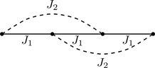
6.5.4.1Next-nearest-neighbor model
The transfer matrix method allows us to treat models having interactions that extend beyond nearest-neighbors.56 We show how to set up the transfer matrix for a model with nearest and next-nearest neighbor interactions,57 with Hamiltonian
H(σ)=−J1∑i=1Nσiσi+1−J2∑i=1Nσiσi+2,
(6.102)
where we adopt periodic boundary conditions, σN+1≡σ1 and σN+2≡σ2. Figure 6.23 shows the two types of interactions and their connectivity in one dimension.
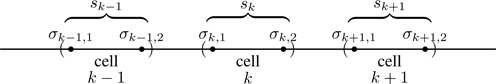
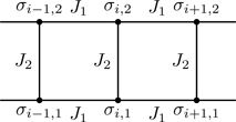
To set up the transfer matrix, we group spins into cells of two spins apiece, as shown in Fig. 6.24. We label the spins in the kth cell (σk,1,σk,2), 1≤k≤N/2. A key step is to associate the degrees of freedom of each cell with a new variable sk representing the four configurations (+,+),(+,−),(−,+),(−,−). This is a mapping from the 2N degrees of freedom of Ising spins {σi}, 1≤i≤N, to an equivalent number 4N/2 degrees of freedom associated with the cell variables {sk}, 1≤k≤N/2.
Figure 6.24Grouping of spins into cells of two spins apiece.
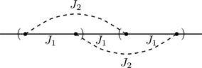
Besides grouping spins into cells, we also classify interactions as those associated with intra-cell couplings (see Fig. 6.25)
With these definitions, the Hamiltonian can be written as the sum of two terms, one containing all intra-cell interactions and the other containing all inter-cell interactions,
H(s)=∑k=1N/2V0(sk)+V1(sk,sk+1)≡H0(s)+H1(s),
(6.105)
where s(N/2)+1≡s1. Comparing Eqs. (6.102) and (6.105), we see that all interactions of the model are accounted for; we have simply rewritten the Hamiltonian by grouping the spins into cells.58
Figure 6.25Intra- and inter-cell spin couplings.
The partition function, expressed in terms of cells variables, is then
where Ki=βJi, i=1,2, and ∑{s}≡∑s1⋯∑sN/2 indicates a summation over cell degrees of freedom. In analogy with the step between Eqs. (6.76) and (6.77), we can write Eq. (6.106)
and where {λi}i=14 are its eigenvalues. Clearly T is a 4×4 matrix because the sums in Eq. (6.107) are over the four degrees of freedom represented by the variable sk. The explicit form of T is
The matrix in Eq. (6.109) is in block-symmetric form A\BB\A because of the order with which we’ve written the basis elements in Eq. (6.109) with up-down symmetry. Explicit expressions for the eigenvalues of T are (after some algebra),
The partition function ZN(K1,K2) follows by combining Eq. (6.110) with Eq. (6.107).
If we set K1=0, the system separates into two inter-penetrating yet uncoupled sublattices, where, within each sublattice, the spins interact through nearest-neighbor couplings. Using the eigenvalues in Eq. (6.110), we have from Eq. (6.107),
ZN(0,K2)=2coshK2N/2+2sinhK2N/22=ZN/2nn(K2)2,
(6.111)
where Znn is the partition function for the nearest-neighbor model (in zero magnetic field), Eq. (6.80). Equation (6.111) illustrates the general result that the partition function of noninteracting subsystems is the product of the subsystem partition functions. If we set K2=0, we’re back to the N-spin nearest-neighbor Ising model in zero magnetic field. It’s readily shown that59
ZN(K1,0)=ZNnn(K1).
(6.112)
6.5.4.2Further-neighbor interactions
It’s straightforward to generalize to a one-dimensional system with arbitrarily distant interactions.60 Define an N-spin model with up to pth-neighbor interactions, where p is arbitrary,
H(σ)=−∑m=1p∑k=1NJmσkσk+m,
(6.113)
where we invoke periodic boundary conditions, σN+m≡σm, 1≤m≤p. Clearly we should have N≫p for such a model to be sensible.
We break the system into cells of p contiguous spins,61(σk,1,σk,2,⋯,σk,p), 1≤k≤N/p. We associate the 2p spin configurations of the kth cell with the symbol sk. The transfer matrix will then be a 2p×2p matrix. We rewrite the Hamiltonian, making the distinction between intra- and inter-cell couplings,
V0(sk)=−∑m=1p−1∑j=1p−mJmσk,jσk,j+m
(6.114)
V1(sk,sk+1)=−∑m=0p−1∑j=1p−mJp−mσk,j+mσk+1,j,
(6.115)
so that
H(s)=∑k=1N/pV0(sk)+V1(sk,sk+1)≡H0(s)+H1(s).
(6.116)
Equations (6.103) and (6.104) are special cases of Eqs. (6.114) and (6.115) with p=2. By counting terms in Eqs. (6.114) and (6.115), there are p(p−1)/2 intra-cell couplings and p(p+1)/2 inter-cell couplings for a total of p2 couplings associated with each cell. The total number of spin interactions is thus preserved by the grouping of spins into cells. The Hamiltonian Eq. (6.113) represents a total of Np spin interactions, the same number represented by Eq. (6.116): Np=(N/p)p2. The division into cells also preserves the number of spin configurations: 2N=2p(N/p).
To complete the discussion, the partition function for the pth-neighbor model is
where (λ1,⋯,λ2p) are the eigenvalues of the matrix T(s,s′)=exp(−βV0(s))exp(−βV1(s,s′)).
6.5.4.3The Ising spin ladder
We now apply the transfer matrix to a more complicated one-dimensional system shown in Fig. 6.26, a “ladder” of 2N Ising spins satisfying periodic boundary conditions. To set up the transfer matrix, which groups of spins can we treat as adjacent cells? With the spins labeled as in Fig. 6.26, the Hamiltonian can be written
H=−J2∑i=1Nσi,1σi,2−J1∑i=1Nσi,1σi+1,1+σi,2σi+1,2.
(6.118)
Figure 6.26A 2×N Ising model with couplings J1 and J2.
The transfer matrix is therefore
T(σ,σ′)=eK2σ1σ2eK1(σ1σ1′+σ2σ2′).
(6.119)
We can write the elements of T(σ,σ′) as we did in Eq. (6.109),
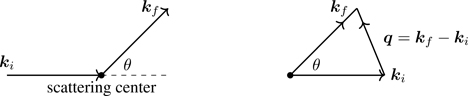
Much of what we know about macroscopic systems comes from scattering experiments. In X-ray scattering, electromagnetic radiation scatters from charges in the system; in neutron scattering, neutrons scatter from magnetic moments in the system (see Appendix E). Figure 6.27 shows the geometry of a scattering experiment. A beam of monochromatic radiation of wave vector ki and angular frequency ω is incident upon a sample and is scattered towards a detector in the direction of the outgoing wave vector kf at angle θ relative to ki. If the energy ℏω is much larger than the characteristic excitation energies of the molecules of the system, scattering occurs without change of frequency (elastic scattering, our concern here) and thus kf has magnitude |kf|=|ki|. In elastic scattering, the wave vector transfer
q≡kf−ki
(6.121)
Figure 6.27Scattering geometry: Incoming and outgoing wave vectors ki,kf with q=kf−ki.
has magnitude |q|=2|ki|sin(θ/2). A record of the scattering intensity as a function of θ provides one with the Fourier transform of the two-particle correlation function (as we’ll show), the static structure factor.62
Assume, for a particle at position rj (relative to an origin inside the sample) that an incident plane wave with amplitude proportional to eiki·rj is scattered into an outgoing spherical wave63 centered at rj. The amplitude of the scattered wave at the detector at position R is proportional to
αeiki·rjeikfR−rjR−rj,
(6.122)
where kf≡kf and α is the scattering efficiency64 of the particle at rj. The detector is far removed from the sample with R≡R≫rj≡rj (for all j), implying that R−rj≈R−R^·rj, where R^≡R/R (show this). In the denominator of (6.122) we can approximate R−rj≈R, but not in the phase factor. With kf=kfR^, we have for the amplitude at the detector:
eiki·rjeikfR−rjR−rj≈eikfRRe−iq·rj,
where q is defined in Eq. (6.121). The detector receives scattered waves from all particles of the sample, and thus the total amplitude A at the detector is
A=A0∑je−iq·rj,
(6.123)
where A0 includes eikfR/R, together with any other constants we’ve swept under the rug. The intensity at the detector is proportional to the square of the amplitude, I∝A2. Data is collected in scattering experiments over times large compared with microscopic time scales associated with fluctuations, and thus what we measure is the ensemble average,
provisionally defines the static structure factor (see Eq. (6.130)). Note the separation that Eq. (6.124) achieves between I0, which depends on details of the experimental setup, and S(q), the intrinsic response of the system.
Let’s momentarily put aside Eq. (6.125). Define the instantaneous local density of particles,
n(r)≡∑j=1Nδr−rj.
(6.126)
The reader should understand how Eq. (6.126) works: The three-dimensional Dirac delta function has dimension V−1, where V is volume. In summing over the positions rj of all particles in Eq. (6.126), the delta function counts65 the number of particles at r, and hence we have the local number density, n(r). Its Fourier transform is66
n(q)≡∫e−iq·rn(r)d3r=∑je−iq·rj,
(6.127)
where we’ve used Eq. (6.126). Note that n(q)*=n(−q). By substituting Eq. (6.127) in Eq. (6.125), we have an equivalent expression for the structure factor,
The scattering intensity (into the direction associated with q) is therefore related to the Fourier transform (at wave vector q) of the correlation function, 〈n(r′)n(r)〉. Given enough scattering measurements, the complete Fourier transform can be established, which can be inverted to find the correlation function. The point here is that the two-particle correlation function can be measured.
Equation (6.128) has a flaw that’s easily fixed. Define local density fluctuations δn(r)≡n(r)−〈n(r)〉=n(r)−n, where n≡N/V is the average density (which because of translational invariance is independent of r).67 Note that 〈δn(r)〉=0. Substituting n(r)=n+δn(r) in Eq. (6.128),
S(q)=1N∫∫d3rd3r′eiq·(r′−r)〈δn(r′)δn(r)〉+8π3nδ(q),
(6.129)
where we’ve used the integral representation of the delta function, ∫−∞∞eiqxdx=2πδ(q). The presence of δ(q) in Eq. (6.129) indicates a strong signal in the direction of q=0, the forward direction defined by kf=ki. Because radiation scattered into the forward direction cannot be distinguished from no scattering at all, we cannot expect S(q) as given by Eq. (6.129) to represent scattering data at q=0. It’s conventional to subtract this term, redefining S(q),
S(q)≡1N∫∫d3rd3r′eiq·(r′−r)〈δn(r′)δn(r)〉.
(6.130)
The out-of-beam scattering intensity at q≠0 is therefore related to the Fourier transform of the correlation function of fluctuations, 〈δn(r′)δn(r)〉. The extent to which spatially separated local fluctuations are correlated determines the scattering strength.
The value of S(q) as q→0 is, from Eq. (6.130) (after subtracting the delta function),
where we’ve used Eq. (4.81) and n=〈N〉/V. Thus, S(q=0) represents long-wavelength, thermodynamic fluctuations in the total particle number, 〈N−〈N〉2〉, whereas S(q≠0) represents correlations of spatially separated microscopic (local) fluctuations, 〈δn(r)δn(r′)〉.
Example. Evaluate S(q) for the one-dimensional, nearest-neighbor Ising model in zero magnetic field, using Eq. (6.99) for the correlation functions. From Eq. (6.130), using sums over lattice sites instead of integrals, we have (where a is the lattice constant)
where we’ve let N→∞, we’ve used translational invariance, and we’ve introduced the abbreviation u≡tanhK. S(q) is peaked at q=0 for K>0, and at q=±π/a for K<0. It’s straightforward to show that S(q=0)=χ, where the susceptibility χ is given in Eq. (6.86).
The structure factor can be written in yet another way by returning to Eq. (6.125) and recognizing that eiq·rk−rj=∫d3reiq·rδr−(rk−rj). Thus we have the equivalent expression
S(q)=1N∫d3reiq⋅r〈∑j∑kδ(r−(rk−rj))〉.
(6.133)
Separate the terms in the double sum for which k=j:
〈∑j∑kδ(r−(rk−rj))〉=Nδ(r)+〈∑j∑k≠jδ(r−(rk−rj))〉.
(6.134)
The second term on the right of Eq. (6.134) defines the radial distribution function,
ng(r)=1N〈∑j∑k≠jδ(r−(rk−rj))〉.
(6.135)
where n (density) is included in the definition to make g(r) dimensionless. The delta functions in Eq. (6.135) count the number of pairs of particles that are separated by r. If the system is isotropic, g(r) is a function only of r: g=g(r). Because of translational invariance,68 the definition in Eq. (6.135) is equivalent to69 (taking rj as the origin) ng(r)=∑k≠0〈δ(r−rk)〉. As r→∞ the sum captures all particles of the system and g(r)→1. Combining Eqs. (6.135) and (6.134) with Eq. (6.133),
S(q)=1+n∫d3reiq·rg(r).
(6.136)
Equation (6.136) suffers from the same malady as Eq. (6.128). So that the Fourier transform in Eq. (6.136) be well defined,70 we add and subtract unity (the value of g as r→∞),
Just as in Eq. (6.129), we subtract the delta function. Thus, another definition of S(q), equivalent to Eq. (6.130), is
S(q)=1+n∫d3reiq·r[g(r)−1].
(6.137)
For an isotropic system,
S(q)=1+4πn∫0∞r2sinqrqrg(r)−1dr.
(6.138)
If the wavelength λ=2π/ki is large compared with the range ξ over which [g(r)−1] is finite, i.e., qξ≪1, one can replace sinqr/(qr) in Eq. (6.138) with unity, in which case the scattering is isotropic—even for systems with correlated fluctuations. The frequency must be chosen so that ℏω is large compared with excitation energies, and the wavelength is small,712πc/ω≪ξ. The extent to which fluctuations are correlated can be probed experimentally only if λ≪ξ. For noninteracting particles, g(r)=1 (as one can show), and the scattered radiation is isotropic with S(q)=1.
To observe scattering from correlated fluctuations requires the wavelength to be smaller than the correlation length, λ≪ξ, and for that reason X-rays are used to probe the distribution of molecules in fluids. Near critical points, however,72 strong scattering of visible light occurs, where a normally transparent fluid appears cloudy or opalescent, a phenomenon known as critical opalescence. The wavelength of visible light is ≈104 times as large as that for X-rays, implying that fluctuations become correlated over macroscopic lengths at the critical point. In 1914, L.S. Ornstein and F. Zernike made an important step in attempting to explain the development of long-range, critical correlations,73 one that’s relevant to our purposes and which we review here.
Ornstein and Zernike proposed a mechanism by which correlations can be established between particles of a fluid. They distinguished two types of correlation function: c(r), the direct correlation function, a new function, and h(r)≡g(r)−1, termed the total correlation function (with g(r) the radial distribution function, Eq. (6.135)). The direct correlation function accounts for contributions to the correlation between points of a fluid that are not mediated by other particles, such as that caused by the potential energy of interaction, v(r) (see Eq. (6.1)). Ornstein and Zernike posited a connection between the two types of correlation function (referring to Fig. 6.28):
h(r2−r1)=c(r2−r1)+n∫c(r3−r1)h(r2−r3)d3r3.
(6.139)
Equation (6.139) is the Ornstein-Zernike equation. In addition to the direct correlation between particles at r1,r2 (the first term of Eq. (6.139)), the integral sums the influence from all other particles of the fluid at positions r3. The quantity nd3r3 in Eq. (6.139) represents the number of particles in an infinitesimal volume at r3, each “directly” correlated to the particle at r1, which set up the full (total) correlation with the particle at r2. Equation (6.139) is an integral equation74,75 that defines c(r) (given h(r)). The function c(r)can be given an independent definition as a sum of a certain class of connected diagrams,[76, p99] a topic we lack sufficient space to develop.
Figure 6.28Geometry of the Ornstein-Zernike equation.
By taking the Fourier transform of Eq. (6.139) and applying the convolution theorem[16, p111], we find, where c(q)=∫d3reiq·rc(r),
h(q)=c(q)+nc(q)h(q)⇒c(q)=h(q)1+nh(q).
(6.140)
Equation (6.140) indicates that c(q) does not show singular behavior at the critical point.76 From Eq. (6.137), S(q)=1+nh(q), and, because S(q) diverges as q→0 at T=Tc (see Section 7.6), c(q=0) remains finite at T=Tc. Using Eq. (6.131),
1kTnβT=1S(q=0)=11+nh(q=0)=1−nc(q=0)=1−n∫d3rc(r).
(6.141)
Thus, the direct correlation function is short ranged, even at the critical point.77 If we’re interested in critical phenomena characterized by long-wavelength fluctuations (which we will be in coming chapters), approximations made on the short-ranged function c(r) should prove rather innocuous78 (at least that’s the thinking79). Molecular dynamics simulations have confirmed the short-ranged nature of c(r) [79]. An approximate form for c(r) introduced by Percus and Yevick[80] gives good agreement with experiment and displays its short-ranged character:
c(r)≈1−eβv(r)g(r),
so that c(r) vanishes for distances outside the range of the pair potential.80
Because c(q) is well behaved at Tc, it may be expanded in a Taylor series about q=0. For an isotropic system, c(q)=∑k=0∞ckqk, where the coefficients ck are functions of (n,T) and are related to the moments of the real-space correlation function c(r):
The Ornstein-Zernike approximation consists of replacing c(q) with the first two terms of its Taylor series:
c(q)=c0+c2q2+O(q4).
Higher-order terms are dropped because we’re interested in the low-q, long-range behavior. Combining terms,
S(q)=11−nc(q)≈11−nc0+c2q2≡1R02q02+q2,
(6.143)
where R02≡−nc2 and q02≡(1−nc0)/R02. This approximate, small-q form for S(q) is based on the short-range nature of the direction correlation function c(r), that c(q) can be expanded in a power series, and that terms of O(q4) can be ignored. The inverse Fourier transform of Eq. (6.143) leads to an asymptotic form for the total correlation function, valid at large distances:
h(r)~1R02e−q0rr.
(6.144)
Thus, we identify q0≡ξ−1 as the inverse correlation length. We return to Ornstein-Zernike theory in Chapter 7.
Summary
We considered systems featuring inter-particle interactions: The classical gas, the Tonks-Takahashi gas, and the one-dimensional Ising model. We showed how the equation of state of real gases in the form of the virial expansion, Eq. (6.29), and the nature of the interactions giving rise to the virial coefficients, can be derived in the framework of the Mayer cluster expansion, the prototype of many-body perturbation theories. The Tonks gas features a hard-core repulsive potential (required for the existence of the thermodynamic limit), and the Takahashi gas allows nearest-neighbor attractive interactions in addition to a hard core (but only nearest-neighbor interactions). We introduced the Ising model of interacting degrees of freedom on a lattice, and the transfer matrix method of solution. We introduced the correlation length ξ, the characteristic length over which fluctuations are correlated, which plays an essential role in theories of critical phenomena. We discussed how scattering experiments probe the structure of systems of interacting particles, and the approximate Ornstein-Zernike theory of the static structure factor.
EXERCISES
6.1We said in Section 6.1 that perturbation theory can’t be used if the inter-particle potential v(r) diverges as r→0. Why not use the Boltzmann factor e−βv(r) as a small parameter for r→0 ? What’s wrong with that idea for applying perturbation theory to interacting gases?
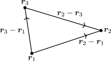
6.2Referring to Fig. 6.29, we have, in calculating the diagram, the integral
I≡∫dr1dr2dr3f(|r1−r2|)f(|r2−r3|)f(|r3−r1|).
Change variables. Let R≡13(r1+r2+r3) be the center-of-mass-coordinate, and let u≡r1−r3, v≡r2−r3. Show that
Hint: Eq. (6.28). The chemical potential is modified relative to the ideal gas, either positively or negatively, depending on the sign of b2.
6.6Derive an expression for the fourth virial coefficient, B4(T), i.e., work out the next contribution to the series in Eq. (6.29). A: −20b23+18b2b3−3b4.
6.7Derive Eq. (6.33) for the second virial coefficient associated with the van der Waals equation of state, B2vdw. What is the expression for B3vdw ? A: b2.
6.8Fill in the steps from Eq. (6.34) to Eq. (6.35) using the Lennard-Jones potential.
6.9Derive Eqs. (6.44), (6.45), and (6.49).
6.10Verify the claim that C3=0 for the diagrams in Fig. 6.14.
6.11Show that C3=0 for the diagram in the right-most part of Fig. 6.15. Hint: Make use of Eq. (6.45).
6.12Derive Eq. (6.53). Hint: Start with P=−∂F/∂VT,N (see Table 1.2) and show that (with n=N/V)
P=n2∂(F/N)∂nT.
Then use the relation −βF=lnZ, Eq. (4.57). Without fanfare, we’ve been working with the canonical ensemble in Section 6.3.
6.13Derive Eqs. (6.59)–(6.62). Then show the thermodynamic limits, Eq. (6.63)
6.14Derive an expression for the internal energy of the Tonks gas. Does your result make sense? Hint: F=U−TS.
6.15Verify the identity shown in Eq. (6.70).
6.16Derive the expressions in Eq. (6.72). Hint: First show that T(∂/∂T)=−K(∂/∂K).
6.17 Show that the heat capacity of one-dimensional Ising spins has the form at low temperature,
CV~T→01T2e−2|J|/(kT),
the same low-temperature form of the heat capacity of rotational and vibrational modes in molecules (see Chapter 5). Compare with the low-temperature heat capacity of free fermions, Eq. (5.106), free massive bosons, Eq. (5.166), and photons, Eq. (5.134).
6.18Find the eigenvalues of the transfer matrix in Eq. (6.79) and show they agree with Eq. (6.82).
6.19Show that the magnetization of the one-dimensional Ising model (see Eq. (6.84)) demonstrates saturation, that 〈σ〉→1 for sinh2B≫1.
6.20Suppose there were no near-neighbor interactions in the Ising model (K=0), but we keep the coupling to the magnetic field. Show that in this case 〈σ〉 reduces to one of the Brillouin functions studied in Section 5.2. Which one is it, and does that make sense?
6.21Find the eigenvalues of the transformed Pauli matrix S˜ in Eq. (6.95). Are you surprised by the result?
6.22Consider the single-spin average in Eq. (6.97) for the finite system (before we take the thermodynamic limit). Suppose N=1, then the resulting expression for 〈σ〉 should be independent of the near-neighbor coupling constant K. Show that the limiting form of Eq. (6.97) for N=1 is the correct expression.
6.23Show in the one-dimensional Ising model for B=0 that ξ diverges for T→0 as,
ξ~T→012exp(2K).
(P6.1)
6.24The Ising partition function for periodic boundary conditions, Eq. (6.80), is the customary result derived using the transfer matrix, so much so one might conclude periodic boundary conditions are essential to the method. That’s not the case, as this exercise shows, where we derive the partition function associated with free boundary conditions, Eq. (6.71), using the transfer matrix.
Start with Eq. (6.68) as the Hamiltonian for free boundary conditions (take b=0 for simplicity). Set up the calculation of the partition function using the transfer matrix:
Clearly, we can’t “wrap around” to take the trace. To finish the calculation, we require a general expression for powers of the transfer matrix.
The transfer matrix V is diagonalizable—there exists a matrix P such that P−1VP=Λ, where Λ is diagonal. That implies V=PΛP−1 (show this). Show that for integer n, Vn=PΛnP−1. Using the transformation matrix in Eq. (6.94) for ϕ=π/4 (zero field), show that
The eigenvalues of the matrix in Eq. (P6.3) (which is symmetric) are the same as those of the matrix in Eq. (6.120) (which is block symmetric)—they describe the same physical system. There must be a similarity transformation between the two matrices.
6.27Show, using Eq. (6.125), that S(q)=S*(q), i.e., the structure factor is a real-valued function. Hint: j,k are dummy indices.