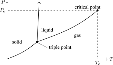
CHAPTER 7 Phase transitions and critical phenomena

PHASE, as the term is used in thermodynamics, refers to a spatially uniform equilibrium system.¹ A body of given chemical composition can exist in a number of phases. H₂O, for example, can exist in the familiar liquid and vapor phases, as well as several forms of ice having different crystal structures. Substances undergo phase transitions, changes in phase that occur upon variations of state variables. Phases can coexist in physical contact (such as an ice-water mixture). Figure 7.1 is a generic phase diagram, the values of T,P for which phases exist and coexist along coexistence curves. Note the triple point, a unique combination of T,P at which three phases coexist.² At the critical point, the liquid-vapor coexistence curve ends at Tc,Pc (critical temperature and pressure), where the distinction between liquid and gas disappears.³ For T>Tc, a gas cannot be liquefied regardless of pressure. In the vicinity of the critical point (the critical region), properties of materials undergo dramatic changes as the distinction between liquid and gas disappears. Lots of interesting physics occurs near the critical point—critical phenomena—basically the remainder of this book.⁴

Figure 7.1Phase diagram in the P–T plane. Thick lines are coexistence curves.

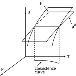
7.1 Phase coexistence, Gibbs phase rule

7.1.1 Equilibrium conditions

We start by asking whether there is a limit to the number of phases that can coexist. An elegant answer is provided by the Gibbs phase rule, Eq. (7.13). The chemical potential of substances in coexisting phases has the same value in each of the phases in which coexistence occurs.⁵ Consider two phases of a substance, I and II. Because matter and energy can be exchanged between phases in physical contact, equilibrium is achieved when T and P are the same in both phases, and when the chemical potentials are equal, μI=μII (see Section 1.12). We know from the Gibbs-Duhem equation,⁶ (P1.1), that μ=μ(T,P), and thus chemical potential can be visualized as a surface μ=μ(T,P) (see Fig. 7.2). Two phases of the same substance coexist when

μI(T,P)=μII(T,P) .

(7.1)

The intersection of the two surfaces defines the locus of points P=P(T) for which Eq. (7.1) is satisfied—the coexistence curve (see Fig. 7.2). Three coexisting phases (I,II,III) would require the equality of three chemical potential functions,

μI(T,P)=μII(T,P)=μIII(T,P) .

(7.2)

Figure 7.2Coexistence curve defined by the intersection of chemical potential surfaces associated with phases I and II of a single substance.

Equation (7.2) implies two equations in two unknowns and thus three phases can coexist at a unique combination of T and P, the triple point. By this reasoning, it would not be possible for four phases of a single substance to coexist (which would require three equations in two unknowns). Coexistence of four phases of the same substance is not known to occur.

Multicomponent phases have more than one chemical species. Let μjγ denote the chemical potential of species j in the γ phase (we use Roman letters to label species and Greek letters to label phases). Assume k chemical species, 1≤j≤k,, and π phases, 1≤γ≤π,, where π is an integer. The first law for multiphase, multicomponent systems is the generalization of Eq. (1.21):

dU=TdS−PdV+∑γ=1π∑j=1kμjγdNjγ .

(7.3)

Extensivity implies the scaling property U(λS,λV,λNjγ)=λU(S,V,Njγ). By Euler’s theorem,

U=S∂U∂SV,Njγ+V∂U∂VS,Njγ+∑γ=1π∑j=1kNjγ∂U∂NjγS,V=TS−PV+∑γ=1π∑j=1kμjγNjγ ,

(7.4)

where the derivatives follow from Eq. (7.3) and Njγ¯ indicates to hold fixed particle numbers except Njγ. Equation (7.4) implies

G=∑γ=1π∑j=1kμjγNjγ ,

(7.5)

the generalization of Eq. (1.54). Taking the differential of Eq. (7.4) and using Eq. (7.3), we have the multicomponent, multiphase generalization of the Gibbs-Duhem equation, (P1.1),

∑γ=1π∑j=1kNjγdμjγ=−SdT+VdP .

(7.6)

By taking the differential of G in Eq. (7.5), and making use of Eq. (7.6),

dG=−SdT+VdP+∑γ=1π∑j=1kμjγdNjγ ,

(7.7)

and thus we have the alternate definition of chemical potential,⁷ μjγ=∂G/∂NjγT,P,Njγ¯, the energy to add a particle of type j in phase γ holding fixed T, P, and the other particle numbers.

The Gibbs energy is a minimum in equilibrium.⁸ From Eq. (7.7),

dGT,P=∑γ=1π∑j=1kμjγdNjγT,P=0 .

(7.8)

If the particle numbers Njγ could be independently varied, one would conclude from Eq. (7.8) that μjγ=0. But particle numbers are not independent. The number of particles of each species spread among the phases is a constant,⁹ ∑γNjγ= constant, and thus there are k equations of constraint

∑γ=1πdNjγ=0 . j=1,⋯,k

(7.9)

Constraints are handled through the method of Lagrange multipliers¹⁰ λ_j, which when multiplied by Eq. (7.9) and added to Eq. (7.8) leads to

∑j=1k∑γ=1πμjγ+λjdNjγ=0 .

(7.10)

We can now treat the particle numbers as unconstrained, so that Eq. (7.10) implies

μjγ=−λj .

(7.11)

The chemical potential of each species is independent of phase. Equation (7.11) is equivalent to

μj1=μj2=⋯=μjπ . j=1,⋯,k

(7.12)

There are k(π−1) equations of equilibrium for k chemical components in π phases.

7.1.2 The Gibbs phase rule

How many independent state variables can exist in a multicomponent, multiphase system? In each phase there are Nγ≡∑j=1kNjγ particles, and thus there are k−1 independent concentrations cjγ≡Njγ/Nγ, where ∑j=1kcjγ=1. Among π phases there are π(k−1) independent concentrations. Including P and T, there are 2+π(k−1) independent intensive variables.

There are k(π−1) equations of equilibrium, Eq. (7.12). The variance of the system is the difference between the number of independent variables and the number of equations of equilibrium,

f≡2+π(k−1)−k(π−1)=2+k−π .

(7.13)

Equation (7.13) is the Gibbs phase rule.[11, p96] It specifies the number of intensive variables that can be independently varied without disturbing the number of coexisting phases ( f≥0).

• k=1,π=1⇒f=2: a single substance in one phase. Two intensive variables can be independently varied; T and P in a gas.

• k=2,π=1⇒f=3: two substances in a single phase, as in a mixture of gases. We can independently vary T, P, and one mole fraction.

• k=1,π=2⇒f=1: a single substance in two phases; a single intensive variable such as the density can be varied without disrupting phase coexistence.

• k=1,π=3⇒f=0: a single substance in three phases; we cannot vary the conditions under which three phases coexist in equilibrium. Unique values of T and P define a triple point.

One should appreciate the generality of the phase rule, which doesn’t depend on the type of chemical components, only that the Gibbs energy is a minimum in equilibrium.

7.1.3 The Clausius-Clapeyron equation

The latent heat, L, is the heat released or absorbed during a phase change, and is measured either as a molar quantity (per mole) or as a specific quantity (per mass). One has the latent heat of vaporization (boiling), fusion (melting), and sublimation.¹¹ Latent heats are also called the enthalpy of vaporization (or fusion or sublimation).¹² At a given T,

L(T)=hv−hl=T sv(T,P(T))−sl(T,P(T)) ,

(7.14)

where v and l refer to vapor and liquid, lower-case quantities such as s≡S/n indicate molar values, and P(T) describes the coexistence curve.¹³ The difference in molar entropy between phases is denoted Δs≡sv−sl; likewise with Δh. Equation (7.14) is written compactly as L=Δh=TΔs.

As we move along a coexistence curve, T and P vary in such a way as to maintain the equality μI(T,P)=μII(T,P). Variations in T and P induce changes δμ in the chemical potential, and thus along the coexistence curve, δμI=δμII. For a single substance, dμ=−sdT+vdP (Gibbs-Duhem equation). At a coexistence curve, −sIdT+vIdP=−sIIdT+vIIdP, implying

dPdTcoexist=sI−sIIvI−vII=ΔsΔv=ΔhTΔv=LTΔv .

(7.15)

Equation (7.15) is the Clausius-Clapeyron equation; it tells us the local slope of the coexistence curve. If one had enough data for L as a function of T, P and the volume change Δv, Eq. (7.15) could be integrated to obtain the coexistence curve in a P–T diagram.

7.2 The classification of phase transitions

Phase coexistence at a given value of (T,P) requires the equality μI(T,P)=μII(T,P), but that says nothing about the continuity of derivatives of μ at coexistence curves. For a single substance, μ=G/N, and thus from Eq. (1.14) (or the Gibbs-Duhem equation (P1.1)),

VN=∂μ∂PT,N SN=−∂μ∂TP,N .

(7.16)

For second derivatives, using Eqs. (1.33) and (P1.6), together with Eq. (7.16),¹⁴

βTN=−1V∂(V/N)∂PT,N=−1V∂2μ∂P2T,NCPN=T∂(S/N)∂TP,N=−T∂2μ∂T2P,N .

(7.17)

The behavior of these derivatives at coexistence curves allows a way to classify phase transitions.

• If the derivatives in Eq. (7.16) are discontinuous at the coexistence curve (i.e., μ(T,P) has a kink at the coexistence curve), the transition is called first order and the specific volume and entropy are not the same between phases, Δv≠0, Δs≠0. The Clausius-Clapeyron equation is given in terms of the change in specific volume Δv and entropy, Δs=L/T. If a latent heat is involved, there are discontinuities in specific volume and entropy, and the transition is first order.

• If the derivatives in Eq. (7.16) are continuous at the coexistence curve, but higher-order derivatives are discontinuous, the transition is called continuous. For historical reasons, continuous transitions are also referred to as second-order phase transitions.¹⁵ At continuous phase transitions, Δv=0 and Δs=0 —there is no latent heat. Entropy is continuous, but its first derivative, the heat capacity, is discontinuous. Whether or not there is a latent heat seems to be the best way of distinguishing phase transitions.

¹³While Eq. (7.14) has been written in terms of the liquid-gas transition, it applies for any two coexisting phases.

¹⁴Because βT,CP>0, the second derivatives in Eq. (7.17) are negative.

¹⁵The Ehrenfest classification scheme, introduced in 1933, proposed to classify phase transitions according to the lowest order of the differential coefficients of the Gibbs function that show a discontinuity. Pippard[82, p137] illustrates how C_P would behave at first, second, and third-order transitions. There’s no reason phase transitions obeying the Ehrenfest scheme can’t occur, yet the idea hasn’t proved useful in practice, other than introducing the terminology of first and second-order phase transitions into the parlance of physics. By focusing only on discontinuities in thermodynamic derivatives, the scheme ignores the possibility of divergences in measurable quantities at phase transitions.

7.3 Van der Waals liquid-gas phase transition

The van der Waals equation of state, (6.32), is a cubic equation in the specific volume, V/N:

VN3−b+kTPVN2+aPVN−abP=0 .

(7.18)

Cubic equations have three types of solutions: a real root together with a pair of complex conjugate roots, all roots real with at least two equal, or three real roots.[50, p17] The equation of state is therefore not necessarily single-valued;¹⁶ it could predict several values of V/N for given values of P and T. For large V/N (how large?—see below), we can write Eq. (7.18) in the form

(VN)2 [VN−(b+kTP)+aN2PV2(VN−b)]=0 .

(7.19)

Large V/N is the regime where the volume per particle is large compared with microscopic volumes, V/N≫a/(kT),b (the van der Waals parameter a has the dimension of energy-volume). In this limit, the nontrivial solution¹⁷ of Eq. (7.19) is the ideal gas law, PV=NkT. For small V/N, we can guess a solution of Eq. (7.18) as V/N≈b (the smallest volume in the problem), valid at low temperature; see Exercise 7.3. (We can’t have V/N=b, which implies infinite pressure.) For V/N≈b, densities approach the close-packing density. We have no reason to expect the van der Waals model to be valid at such densities, yet it indicates a condensed phase, an incompressible form of matter with V/N≈constant, independent of P. At low temperature, kT≪Pb, Eq. (7.18) has one real root, with a pair of complex conjugate roots (see Exercise 7.4).

7.3.1 The van der Waals critical point

Thus, we pass from the low temperature, high density system (low specific volume), in which Eq. (7.18) has one real root, to the high temperature, low density system (large specific volume) which has one nontrivial root (ideal gas law). We shouldn’t be surprised if in between there is a regime for which Eq. (7.18) has multiple roots (which hopefully can be interpreted physically). Detailed studies show there is a unique set of parameters P_c, T_c, and (V/N)c (which as the notation suggests are the pressure, temperature, and specific volume of a critical point¹⁸), at which Eq. (7.18) has a triple root. For (V/N)c≡vc a triple root of Eq. (7.18), the cubic equation

v−vc3=v3−3vcv2+3vc2v−vc3=0

(7.20)

must be equivalent to Eq. (7.18) evaluated at P_c and T_c. Comparing coefficients of identical powers of v in Eqs. (7.18) and (7.20), we infer the correspondences

3vc=b+kTcPc 3vc2=aPc vc3=abPc .

These equations imply the values of the critical parameters (show this):

vc=3b Pc=a27b2 kTc=8a27b .

(7.21)

The relations in Eq. (7.21) predict P_c and T_c reasonably well, but overestimate v_c (Exercise 7.5). Equation (7.21) also predicts Pcvc/(kTc)=38 (show this), a universal number, the same for all gases. In actuality, Pcvc/(kTc)≈0.2 –0.3 for real gases.¹⁹ Should we be discouraged by this disagreement? Not at all! The van der Waals model is the simplest model of interacting gases—if we want better agreement with experiment, we have to include more relevant physics in the model.

7.3.2 The law of corresponding states and the Maxwell equal area rule

Express P, T, and v in units of the critical parameters. Let

P¯≡P/Pc T¯≡T/Tc v¯≡v/vc .

(7.22)

The dimensionless quantities P¯,T¯,v¯ are known as the reduced state variables of the system. With P=PcP¯, T=TcT¯, and v=vcv¯, the van der Waals equation of state can be written (show this)

(P¯+3v¯2) (3v¯−1)=8T¯.

(7.23)

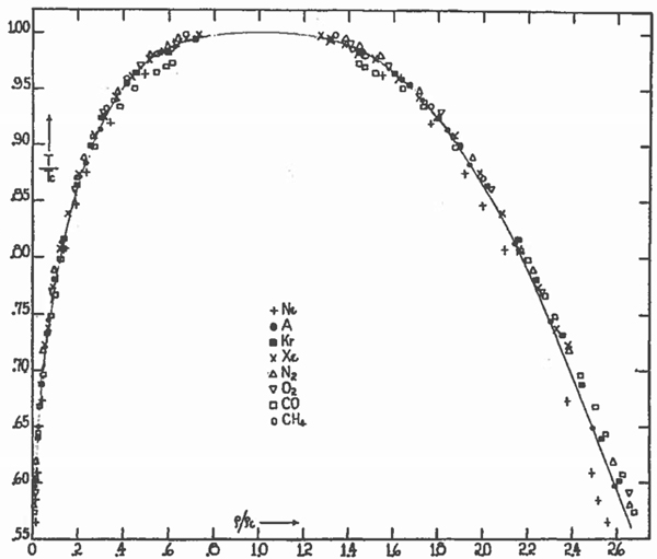
Equation (7.23) is a remarkable development: It’s independent of material-specific parameters, indicating that when P, T, v are scaled in units of P_c, T_c, v_c (which are material specific), the equation of state is the same. Systems having their own values of (a,b), yet the same values of P¯, T¯, v¯, are said to be in corresponding states. Equation (7.23) is the law of corresponding states: Systems in corresponding states behave the same. Thus, argon at T=300 K, for which Tc=151 K, will behave the same as ethane (C₂H₆) at T=600 K, for which Tc=305 K (both have T¯≈2).²⁰ Figure 7.3 is a compelling illustration of the law of corresponding states. For ρ_l (ρ_g) the density of liquid (vapor) in equilibrium at T<Tc, by the law of corresponding states we expect ρl/ρc and ρg/ρc to be universal functions of T/Tc, where ρ_c denotes the critical density. Figure 7.3 shows data for eight substances (of varying complexity²¹ from noble-gas atoms Ne, Ar, Kr, and Xe, to diatomic molecules N₂, O₂, and CO, to methane, CH₄), which, when plotted in terms of reduced variables, ostensibly fall on the same curve![83] The solid line is a fit to the data points of Ar (solid circles) assuming the critical exponent β=13 (see Section 7.4). Figure 7.3 shows the coexistence region—values of temperature and density for which phase coexistence occurs.²²

Figure 7.3The law of corresponding states. Coexistence regions are the same when plotted in terms of reduced state variables. Reproduced from E.A. Guggenheim, J. Chem. Phys. 13, p. 253 (1945), with the permission of AIP Publishing.

Because the equation of state is predicted to be the same for all systems (when expressed in reduced variables), any thermodynamic properties derived from it are also predicted to be the same. Universality is the term used to indicate that the behavior of systems near critical points is largely independent of the details of the system.²³ Universality has emerged as a key aspect of modern theories of critical phenomena, as we’ll see in Section 8.4.²⁴

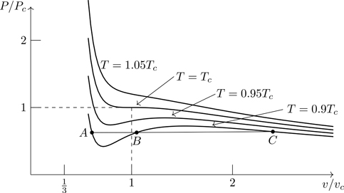
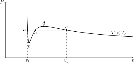
Figure 7.4 shows the isotherms calculated from Eq. (7.23). For T≥Tc, there is a unique specific volume for every pressure—the equation of state is single valued.²⁵ For T<Tc, however, there are three possible volumes associated with a given pressure, such as the values of v/vc shown at A,B,C for T=0.9Tc. How do we interpret these multiple solutions?

¹⁹Values of T_c, P_c, v_c are listed in [57, pp6-37–6-51], from which one can calculate Pcvc/(kTc).

²⁰Note that comparisons of temperatures such as these are possible only when working with absolute temperature.

²¹Note that H and He are not included Fig. 7.3. The law of corresponding states holds for systems in which the distinction between Fermi-Dirac and Bose-Einstein statistics has a negligible effect. It also does not apply to highly polar molecules.

²²The coexistence curve in Fig. 7.1 is the projection of the coexistence region (in the P–v plane) onto the P–T plane.

²³Experimental evidence for universality is presented in the review article of Kadanoff et al [84].

²⁴The occurrence of universality in the van der Waals model illustrates a general process: Discoveries applicable to a wide range of physical systems are often made through specific examples. Entropy was discovered through an analysis of the efficiency of heat engines, yet it’s not restricted to heat engines—it’s a universal feature of the physical world, applying to all forms of matter (solid, liquid, gas), but also to such disparate systems as information and black holes. Experimentally, the law of corresponding states applies to fluids that do not obey the van der Waals equation of state; the law of corresponding states is a more comprehensive theory. We note the distinction between the law of corresponding states, which applies anywhere on a phase diagram, and universality, which concerns systems near critical points.

²⁵From the Gibbs phase rule, two intensive variables can be freely varied for a single-component gas—T and P; the density is uniquely determined by the equation of state.

Figure 7.5 shows an expanded view of an isotherm for T<Tc. We note that (∂P/∂v)T is positive along the segment bcd, which is unphysical. An increase in pressure upon an isothermal expansion would imply a violation of the second law of thermodynamics. The root c in Fig. 7.5 (or B in Fig. 7.4) is unphysical and can be discarded.

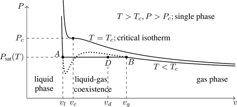
What to make of the other two roots? Figure 7.6 indicates what we expect phenomenologically and hence what we want from a model of phase transitions. As a gas is compressed, pressure rises.²⁶ When (for T<Tc) the gas has been compressed to point B, condensation first occurs (coalescence of gas-phase atoms into liquid-phase clusters). At B, the specific volume v_g represents the maximum density a gas can have at T<Tc. Upon further isothermal compression, the pressure remains constant along the horizontal segment AB (at the saturation pressure, Psat(T)) as more gas-phase atoms are absorbed into the liquid phase.²⁷ At point A, when all gas-phase atoms have condensed into the liquid, the specific volume v=vl is the minimum density a liquid can have at T<Tc. Further compression at this point results in a rapid rise in pressure.

At a point in the coexistence region, such as point D in Fig. 7.6, there are N_l atoms in the liquid phase and N_g in the vapor phase, where N=Nl+Ng is the total number of atoms. Let xl≡Nl/N and xg≡Ng/N denote the mole fractions of the amount of material in the liquid and gas phases. Clearly xl+xg=1. The volume occupied by the gas (liquid) phase at this temperature is Vg=Ngvg ( Vl=Nlvl), implying V=Ngvg+Nlvl. The specific volume v_d associated with point D is:²⁸

vd=VN=Ngvg+NlvlN=xgvg+xlvl=vd (xg+xl),

(7.24)

implying

xlvd−vl=xgvg−vd .

(7.25)

Equation (7.25) is the lever rule.²⁹ As vd→vg, xl→0, and vice versa. See Exercise 7.7.

Note that points A and B in Fig. 7.6, which occur at separate volumes in a P–v phase diagram, are, in a P–T phase diagram (such as Fig. 7.1), located at the same point on a coexistence curve. Along AB in Fig. 7.6, μl(T,P,vl)=μg(T,P,vg), and therefore from Ndμ=−SdT+VdP (Gibbs-Duhem), dμ=0 (phase coexistence) and dT=0 (isotherm) implies dP=0. A horizontal, subcritical isotherm in a P–v diagram indicates liquid-gas coexistence. From the Gibbs phase rule, for a single substance in two phases, one intensive variable (the specific volume) can be varied and not disrupt phase coexistence.

The van der Waals model clearly does not have isotherms featuring horizontal segments. In 1875, Maxwell suggested a way to reconcile undulating isotherms with the requirement of phase coexistence [85]. From the Gibbs-Duhem equation applied to an isotherm ( dT=0), Ndμ=VdP, and thus for an isotherm to represent phase coexistence, we require

0=μl−μg=∫lgdμ=∫lgvdP=∫lg[d (Pv)−Pdv]=(Pv)|lg−∫lgPdv ,

(7.26)

implying

Psat(T) (vg−vl)=∫lgP(v)dv .

(7.27)

Equation (7.27) is the Maxwell equal area rule. It indicates that v_l, v_g, and Psat(T) should be chosen so that the area under the curve of an undulating isotherm is the same as the area under a horizontal isotherm.³⁰ Maxwell in essence modified the van der Waals model so that it describes phase coexistence:

P(v)=kTv−b−av2T≥Tc,all v;T<Tc,v>vg,v<vlPsat(T)T<Tc,vl<v<vg .

(7.28)

The Maxwell rule is an ad hoc fix that allows one to locate the coexistence region in a P–v diagram. One could object that it uses an unphysical isotherm to draw physical conclusions. It’s not a theory of phase transitions in the sense that condensation is shown to occur from the partition function.³¹ In an important study, Kac, Uhlenbeck, and Hemmer showed rigorously that a one-dimensional model with a weak, long-range interaction (in addition to a hard-core, short-range potential), has the van der Waals equation of state together with the Maxwell construction.[88] This work was generalized by Lebowitz and Penrose to an arbitrary number of dimensions.[89] Models featuring weak, long-range interactions are known as mean field theories (Section 7.9); the van der Waals-Maxwell model is within a class of theories, mean field theories. The energy per particle of the van der Waals gas is modified from its ideal-gas value ( 32kT) to include a contribution that’s proportional to the density, −an, the hallmark of a mean-field theory; see Exercise 7.8.

7.3.3 Heat capacity of coexisting liquid-gas mixtures

At a point in the coexistence region (such as D in Fig. 7.6), the total internal energy of the system,

U=Nlul+Ngug ,

(7.29)

where u_l (u_g) is the specific energy, the energy per particle u≡U/N, of the liquid (gas) phase at the same pressure and temperature as the coexisting phases.³² Dividing Eq. (7.29) by N,

u=xlul+xgug .

(7.30)

Compare Eq. (7.30) with Eq. (7.24), which has the same form.

To calculate the heat capacity it suffices to calculate the specific heat, c≡C/N. Starting from CV=∂U/∂TV,N (Eq. (1.38)), the specific heat cv≡CV/N=∂u/∂Tv, where v=V/N. One might think it would be a simple matter to find c_v by differentiating Eq. (7.30) with respect to T, presuming that the mole fractions xl,xg are temperature independent. The mole fractions, however, vary with temperature at fixed volume. As one increases the temperature along the line associated with fixed volume v_d in Fig. 7.6, xl,xg vary because the shape of the coexistence region changes with temperature; consider the lever rule, Eq. (7.25). Of course, dxl=−dxg because of the constraint xl+xg=1. We have, using Eq. (7.30),

cv=(∂u∂T)v=xl(∂ul∂T)coex+xg(∂ug∂T)coex−(ug−ul)(∂xl∂T)coex ,

(7.31)

where ∂/∂Tcoex indicates a derivative taken at the sides of the coexistence region.³³ Evaluating these derivatives is relegated to Exercise 7.10. The final result is:

cv=xlcvl−T∂P∂vlT∂vl∂Tcoex2+xgcvg−T∂P∂vgT∂vg∂Tcoex2 .

(7.32)

Equation (7.32) is a general result, not specific to the van der Waals model.

7.4 A bestiary of critical exponents: α,β,γ,δ

As T approaches T_c from below, T→Tc−, the specific volumes v_g, v_l of coexisting gas and liquid phases tend to v_c, which we can express mathematically as (vg−vc)→0, (vc−vl)→0 as (Tc−T)→0. Can we quantify how vg,vl→vc as T→Tc− ? Because that’s something that can be measured, and calculated from theory. The critical exponent³⁴ β characterizes how vg→vc as T→Tc− through the relation (vg−vc)∝T−Tcβ. Other quantities such as the heat capacity and the compressibility show singular behavior as vg,vl→vc (and the distinction between liquid and gas disappears), and each is associated with its own critical exponent, as we’ll see.

Define deviations from the critical point (which are also referred to as reduced variables)

t≡T−TcTc=T¯−1 ϕ≡v−vcvc=v¯−1 ,

(7.33)

so that t→0− as T→Tc−, and ϕ→0, but can be of either sign as T→Tc−. Substituting T¯=1+t and v¯=1+ϕ into the van der Waals equation of state (7.23), we find, to third order in small quantities,

P¯=1+4t−6tϕ+9tϕ2−32ϕ3+O(tϕ3,ϕ4) .

(7.34)

We’ll use Eq. (7.34) to show that ϕ~|t| as t→0 (see Eq. (7.36)).

7.4.1 Shape of the critical coexistence region, the exponent β

The Maxwell rule can be used to infer an important property of the volumes v_l, v_g in the vicinity of the critical point. From its form in Eq. (7.26), ∫lgvdP=0,

0=∫lgv¯dP¯=∫lg(v¯−1+1) dP¯=∫lgϕdP¯+∫lgdP¯=0∫lgϕ(∂P¯∂ϕ)tdϕ=−∫ϕlϕgϕ (6t+92ϕ2) dϕ ,

(7.35)

where ∫PlPgdP=0 for coexisting phases, we’ve used Eqs. (7.33) and (7.34), and we’ve retained terms up to first order in |t| in ∂P¯/∂ϕt ( ϕ~|t|). The integrand of the final integral in Eq. (7.35) is an odd function of ϕ under ϕ→−ϕ, and the simplest way to ensure the vanishing of this integral for any |t|≪1 is to take ϕl=−ϕg, i.e., the limits of integration are symmetrically placed about ϕ=0. We can make this conclusion only sufficiently close to the critical point where higher-order terms in Eq. (7.34) can be neglected; close to the critical point the coexistence region is symmetric about v_c (which is not true in general—see Fig. 7.3).³⁵

The symmetry P(t,−ϕg)=P(t,ϕg) applied to Eq. (7.34) implies 3ϕg−4|t|+ϕg2=0, or

ϕg=2|t|~T−Tc1/2 . |t|→0

(7.36)

In the van der Waals model, therefore, vg→vc with the square root of T−Tc, and thus it predicts β=12. The measured value of β for liquid-gas critical points is β≈0.32 –0.34[90, 91]. We see from Fig. 7.3 that the coexistence region is well described using β=13.

7.4.2 The heat capacity exponent, α

How does the specific heat behave in the critical region? Let’s approach the critical point along the critical isochore, a line of constant volume, v=vc. As T→Tc−, cvg,cvl→cvc, and xl,xg→12 (use the lever rule and the symmetry of the critical region, vc−vl=vg−vc). From Eq. (7.32),

cv(Tc−)=cv(Tc+)−Tc2limT→Tc− [(∂P∂vl)T(∂vl∂T)coex2+(∂P∂vg)T(∂vg∂T)coex2] ,

(7.37)

where we’ve set cv(Tc+)≡12 (cvl+cvg) as the limit T→Tc+, i.e., the terms in square brackets disappear for T>Tc. For the van der Waals gas, c_v has the ideal-gas value for T>Tc, cv0≡32k (see Exercise 7.8). Equation (7.37) is a general result, and is not specific to the van der Waals model.

For the van der Waals model, we find using Eq. (7.36),

∂v∂Tcoex=∓vcTc1|t| ,

(7.38)

where the upper (lower) sign is for gas (liquid). For the other derivative in Eq. (7.37), we can use Eq. (7.34),

∂P∂vT=Pcvc∂P¯∂ϕt=Pcvc6|t|−18|t|ϕ−92ϕ2=−12Pcvc|t|+O(|t|3/2) ,

(7.39)

where we’ve used Eq. (7.36). From Eq. (7.37), taking the limit,

cv(Tc−)−cv0=−Tc−12Pcvc|t|vcTc21|t|=12PcvcTc=92k ,

where we’ve used Eqs. (7.38) and (7.39), and that Pcvc/Tc=38k (see Eq. (7.21)). Thus,

cv−cv0=92kT→Tc−0T→Tc+ .

(7.40)

The specific heat is discontinuous at the van der Waals critical point—a second-order phase transition in the Ehrenfest classification scheme.

For many systems C_V does not show a discontinuity at T=Tc, it diverges as T→Tc (from above or below),³⁶ such as in liquid ⁴He at the superfluid transition,³⁷ the so-called “λ-transition.” To cover these cases, a heat capacity critical exponent α is introduced,³⁸

CV~T−Tc−α . T→Tc

(7.41)

The value α=0 is assigned to systems showing a discontinuity in C_V at T_c, such as for the van der Waals model. The measured value of α for liquid-gas phase transitions is α≈0.1. Extracting an exponent from measurements can be difficult. If a thermodynamic quantity f(t) shows singular behavior as t→0 in the form f(t)~Atx, the exponent is obtained from the limit

x≡lim⁡t→0ln⁡f(t)ln⁡t .

(7.42)

If x<0, f(t) diverges at the critical point; if x>0, f(t)→0 as T→Tc.

From thermodynamics, CP>CV, Eq. (1.42). The heat capacity C_V for the van der Waals gas is the same as for the ideal gas (Exercise 7.8). C_P, however, has considerable structure for T>Tc; see Eq. (P7.4). In terms of reduced variables, Eq. (P7.4) is equivalent to (show this):

CP−CVNk=(1+ϕ)3(1+t)34ϕ2+ϕ3+t(1+ϕ)3 .

(7.43)

Because ϕ→0 as |t|, Eq. (7.36), we see that C_P diverges as T→Tc+, with

CP~T−Tc−1 . (T→Tc+)

(7.44)

Equation (7.44) is valid for T>Tc; C_P isn’t well defined in the coexistence region.³⁹

7.4.3 The compressibility exponent, γ

We’ve introduced two exponents that characterize critical behavior: α for the heat capacity and β for vg−vl. Is there a γ? One can show that at the van der Waals critical point,

∂P∂v|T=Tc,v=vc=∂2P∂v2|T=Tc,v=vc=0 .

(7.45)

The critical isotherm therefore has an inflection point at v=vc, as we see in Figs. 7.4 or 7.6. The two conditions in Eq. (7.45) define critical points in fluid systems. One can show that

(∂P∂v)t=−2a27b3 [34ϕ2+ϕ3+t(1+ϕ)3(1+ϕ)3(1+32ϕ)2] .

(7.46)

Thus, (∂P/∂v)t~t as t→0. Its inverse, the compressibility βT=−(1/v)(∂v/∂P)T therefore diverges at the critical point,⁴⁰which is characterized by the exponent γ,

βT~T−Tc−γ .

(7.47)

The van der Waals model predicts γ=1; experimentally its value is closer to γ=1.25.

7.4.4 The critical isotherm exponent, δ

The equation of state on the critical isotherm is obtained by setting t=0 in Eq. (7.34), P¯≈1−32ϕ3, implying

P¯−1=P−PcPc=−32v−vcvc3~v−vcvcδ ,

(7.48)

where δ is the conventional symbol for the critical isotherm exponent. The van der Waals model predicts δ=3, whereas for real fluids [91], δ≈4.7 –5.

The definition of the critical exponents α,β,γ,δ and their values are summarized in Table 7.1.

Table 7.1 Critical exponents α,β,γ,δ for liquid-vapor phase transitions
Exponent	Definition	Van der Waals model	Measured
α	CV~T−Tc−α	α=0	α≈0.1
β	vg−vl~T−Tcβ	β=12	β≈0.33
γ	βT~T−Tc−γ	γ=1	γ≈1.25
δ	P−Pc~V−Vcδ	δ=3	δ≈4.7−5

7.5 Weiss molecular field theory of ferromagnetism

We studied paramagnetism in Section 5.2, where independent magnetic moments interact with an external magnetic field. The hallmark of paramagnetism is that the magnetization M vanishes as the applied field is turned off, at any temperature. We saw in the one-dimensional Ising model that adding interactions between spins does not change the paramagnetic nature of that system, Eq. (6.84). Ferromagnets display spontaneous magnetization—a phase transition—in zero applied field, from a state of M=0 for temperatures T>Tc, to one of M≠0 for T<Tc. The two-dimensional Ising model shows spontaneous magnetization (see Section 7.10), so that dimensionality is a relevant factor affecting phase transitions. Indeed, we’ll show that one-dimensional systems cannot support phase transitions (Section 7.12). The two-dimensional Ising model has a deserved reputation for mathematical difficulty. Is there a simple model of spontaneous magnetization?

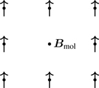
In 1907, P. Weiss introduced a model that bears his name, the Weiss molecular field theory. Figure 7.7 shows part of a lattice of magnetic moments. Weiss argued that if a system is magnetized, the aligned dipole moments of the system would produce an internal magnetic field, B_mol, the molecular field,⁴¹ that’s proportional to the magnetization, Bmol=λM, where the proportionality constant λ will be inferred from the theory. The internal field B_mol would add to the external field, B. Reaching for Eq. (5.18) (the magnetization of independent magnetic moments),

M=N〈μz〉=NμLβμ(B+λM) ,

(7.49)

Figure 7.7Molecular field B_mol is produced by the surrounding magnetic dipoles of the system.

where L(x) is the Langevin function. Equation (7.49) is a nonlinear equation of state, one that’s typical of self-consistent fields where the system responds to the same field that it generates.⁴²

Because we’re interested in spontaneous magnetization, set B=0 in Eq. (7.49):

M=NμL (βμλM) .

(7.50)

Does Eq. (7.50) possess solutions? It has the trivial solution M=0 ( L(0)=0). If Eq. (7.50) is to represent a continuous phase transition, we expect that it has solutions for M≠0. Using the small-argument form of L(x)≈13x−145x3 (see Eq. (P5.1)), Eq. (7.50) has the approximate form for small M,

M≈aM−bM3 ⇒ M1−a+bM2=0 ,

(7.51)

where a≡βNμ2λ/3 and b≡β3μ4Nλ3/45 are positive if λ>0. If a≤1, Eq. (7.51) has the trivial solution. If, however, a>1, it has the nontrivial solution M2≈(a−1)/b. Clearly a=1 represents the critical temperature. Let⁴³

kTc≡13Nμ2λ ⇒ λ=3kTcNμ2 .

(7.52)

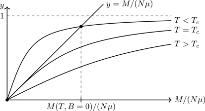
Combining Eqs. (7.52) and (7.50), and letting y≡M/(Nμ), we have the dimensionless equation:

y=L3TcTy .

(7.53)

Figure 7.8 shows a graphical solution of Eq. (7.53). For T≥Tc, there is only the trivial solution, whereas for T<Tc, there is a solution with M≠0 for B=0. Spontaneous magnetization thus occurs in the Weiss model. Just as with liquid-vapor phase transitions, exponents characterize the critical behavior of magnetic systems. We now consider the critical exponents of the Weiss model.

7.5.1 The magnetization exponent, β

To find β is easy—it’s implied by Eq. (7.51) for T<Tc. In the limit T→Tc−,

M2=(53N2μ2) (Tc−TTc) ~ (Tc−TTc)2β , (T→Tc−)

(7.54)

implying β=12 for the Weiss model. Experimental values of β for magnetic systems are in the range 0.30–0.325[94, 95].

7.5.2 The critical isotherm exponent, δ

At T=Tc, M→0 as B→0; the vanishing of M in characterized by the critical exponent δ, defined as B~Mδ at T=Tc. To extract the exponent, we need to “dig out” B from the equation of state, Eq. (7.49), for small M. Combining Eq. (7.52) with Eq. (7.49), where y=M/(Nμ),

y=LβμB+3TcTy .

(7.55)

We can isolate the field term B in Eq. (7.55) by invoking the inverse Langevin function L−1(y):

βμB=L−1(y)−3TcTy .

(7.56)

A power series representation of L−1 can be derived from the Lagrange inversion theorem [50, p14], where for −1<y<1,

L−1(y)=∑k=1∞ykk!dk−1dxk−1xL(x)kx=0≡∑k=1∞ckyk=3y+95y3+297175y5+O(y7) .

(7.57)

Additional coefficients c_k are tabulated in [96]. Combining the small-y form of L−1 from Eq. (7.57), with Eq. (7.56), we find

βμB=3t1+ty+95y3+O(y5) ,

(7.58)

where t is defined in Eq. (7.33). On the critical isotherm t=0, and thus from Eq. (7.58),

B=(9kTc5μ) (MNμ)3 . (|M|≪Nμ)

(7.59)

Equation (7.59) should be compared with Eq. (7.48), the analogous result for fluids. The Weiss model predicts δ=3, whereas experimentally δ≈4 –5.

7.5.3 The susceptibility exponent, γ

The magnetic susceptibility χ=(∂M/∂B)T, see Eq. (1.50), is the magnetic analog of the compressibility of fluids, Eq. (1.33). For small M, we have by implicitly differentiating Eq. (7.58),

βμ=t1+t1Nμχ+OM2χ .

We defined χ in Eq. (1.50) as the isothermal susceptibility, but the value of B was unrestricted. What’s usually referred to as the magnetic susceptibility is the zero-field susceptibility. As T→Tc,

χ=∂M∂BT,B=0=Nμ23k1T−Tc≡CT−Tc~T−Tc−γ ,

(7.60)

where C=Nμ2/(3k) is the Curie constant⁴⁴ for this system (see Section 5.2). Equation (7.60) is the Curie-Weiss law;⁴⁵ it generalizes the Curie law, Eq. (5.15), M=CH/T. The Weiss model predicts γ=1.

7.5.4 The heat capacity exponent, α

From the Helmholtz energy F=U−TS and the magnetic Gibbs energy Gm=F−BM (see Section 1.9), we have the identities (using dU=TdS+BdM)

S=−∂F∂TM B=∂F∂MTS=−∂Gm∂TB M=−∂Gm∂BT .

(7.61)

Combining Eqs. (P1.13) and (P1.14) with the results in Eq. (7.61),

CM=T∂S∂TM=−T∂2F∂T2MCB=T∂S∂TB=−T∂2Gm∂T2B .

(7.62)

Which formula⁴⁶ should be used to calculate the heat capacity in the Weiss model?

Equation (7.58) is a power series for B(M), which when combined with B=∂F/∂MT (Eq. (7.61)) provides an expression that can be integrated term by term:

B=∂F∂MT=1βμ3t1+ty+9kT5μy3+O(y5)=3kNμ2(T−Tc)M+9kT5μ1(Nμ)3M3+O(M5) ,

implying,

F(T,M)=F0(T)+3k2Nμ2(T−Tc)M2+9kT20μ1(Nμ)3M4+O(M6) ,

(7.63)

where F0(T) is the free energy of the non-magnetic contributions to the equilibrium state of the system “hosting” the magnetic moments (and which cannot be calculated without further information about the system).

For T≥Tc, M=0, and for T≲Tc, M² is given by Eq. (7.54), so that, from Eq. (7.63),

F(T)={F0(T)T≥TcF0(T)−52NkTct2T→Tc− .

(7.64)

Using Eq. (7.62),

CM−C0=0T≥Tc5NkT→Tc− .

(7.65)

where C⁰ is the heat capacity of the non-magnetic degrees of freedom. Thus, there is a discontinuity in C_M for the Weiss model.

The critical exponent α for magnetic systems is, by definition, associated with C_B (not C_M) as B→0,

CB=0~T−Tc−α .

(7.66)

One might wonder why C_B is used to define the exponent α, given the correspondence with fluid systems V↔M, −P↔B. For T≥Tc, B=0 implies M=0, and for T<Tc the “two phase” M=0 heat capacity also corresponds to B=0 because with ferromagnets there is up-down symmetry. For fluids, we considered the heat capacity of coexisting phases, each of which has a different heat capacity; see Eq. (7.32). For the Weiss model, we can use Eq. (1.51) to conclude that C_B also has a discontinuity at the critical point. Thus, α=0 for the Weiss model.

The critical exponents of the Weiss model have the same values as those in the van der Waals model. Magnets and fluids are different physical systems, yet they have the same critical behavior. Understanding why the critical exponents of different systems can be the same is the central issue of modern theories of critical phenomena; see Chapter 8. Before proceeding, we introduce two more exponents that are associated with correlations in the critical region.⁴⁷

7.6 The critical correlation exponents: ν,η

The long-wavelength limit of the static structure factor for fluids is related to a thermodynamic quantity, β_T, Eq. (6.131) (there is a similar relation for magnets involving χ):

lim⁡q→0S(q)=nkTβT .

(7.67)

As T→Tc, βT→∞, Eq. (7.47), and thus S(q=0)=N−1∫∫d3rd3r′〈δn(r)δn(r′)〉 diverges⁴⁸ as T→Tc, indicating that fluctuations become correlated over macroscopic distances,⁴⁹ even though inter-particle interactions are short ranged. The Ornstein-Zernike equation (6.139) is a model of how long-range correlations can develop through short-range interactions.⁵⁰

The correlation function has the asymptotic form (Ornstein-Zernike theory, Eq. (6.144)),

g(r)~1R02e−r/ξr ,

(7.68)

where R02=−nc2 and the correlation length ξ=R0/1−nc0, with c₀, c₂ moments of the direct correlation function c(r), Eq. (6.142), c0=∫c(r)d3r and c2=−16∫r2c(r)d3r. At the critical point, c0→1/n, Eq. (6.141). Because R₀ is finite at the critical point,⁵¹ we conclude that ξ→∞ as T→Tc. The divergence of ξ as T→Tc is characterized by another critical exponent, ν, with

⁴⁷Critical phenomena—the behavior of physical systems near critical points—are characterized by six numbers: α,β,γ,δ,ν,η. Six numbers isn’t so bad—you learned the alphabet at some point in your life. If you want to do research in this field, you’ll need to know these numbers for a handful of representative systems.

⁴⁸The integrals in Eq. (6.131) are over an infinite volume (thermodynamic limit), yet they usually give finite results because the correlation function quickly decays to zero outside the correlation length ξ.

⁴⁹And of course that’s consistent with the interpretation of critical opalescence. See Section 6.7.

⁵⁰Here’s an urban analogy: Imagine a barking dog in your neighborhood. The audible range of a dog bark is finite, yet if the density of dogs in the town is sufficiently great, dog barking can become correlated over large distances.

ξ~T−Tc−ν .

(7.69)

Like all critical exponents, ν has been introduced phenomenologically. Within the confines of Ornstein-Zernike theory, ν can be related to the exponent γ. Using Eq. (6.141), we find

ξ2=R02kTnβT , (Ornstein-Zernike)

(7.70)

and thus, using Eqs. (7.47) and (7.69), 2ν=γ. This relation does not hold in general, however.

In Ornstein-Zernike theory, S(q) has the form (from Eq. (6.142)),

S(q,T)=R0−2ξ−2+q2+O(q4) .

(7.71)

At T=Tc, S(q) diverges as q→0. This divergence is characterized by another (our final) critical exponent, η, such that

S(q,T=Tc)~q−2+η .

(7.72)

Clearly in the Ornstein-Zernike model, η=0. If one could always ignore the higher-order terms in Eq. (7.71) (the Ornstein-Zernike approximation), one would always have η=0. It’s found, however, that this is not justified in general. The necessity for introducing η is based on a more rigorous analysis of the correlation function that results from the inverse Fourier transform of the Ornstein-Zernike structure factor, particularly in regard to the role of the spatial dimension, d. There are two regimes:[97, p106]

r≫ξ. For fixed T>Tc (and thus finite ξ), we have the asymptotic result for r→∞,

g(r)~e−r/ξr(d−1)/21+Od−3r/ξ ,

(7.73)

which clearly is of the form of Eq. (7.68) for d=3.
ξ≫r. For fixed r, as T→Tc+ (and hence as ξ gets large),

g(r)~(ln⁡r)e−r/ξd=2e−r/ξrd−2d≥3 .

(7.74)

The two limiting forms agree for d=3, with g(r)~e−r/ξ/r. They do not agree for d>3, however. It would be natural to ask, who cares about dimensions higher than three? In the subject of critical phenomena it pays to understand the role of dimension, as we’ll see. Something is clearly amiss for d=2. For T=Tc ( ξ→∞), Eq. (7.74) indicates that correlations in a two-dimensional fluid would increase with distance, which is unphysical; Ornstein-Zernike theory breaks down in two dimensions. A qualitative conclusion from Eq. (7.74) (for d≠2) is that at T=Tc, correlations decay with distance inversely as a power of r: For T≠Tc, correlations decay exponentially; for T=Tc, correlations decay algebraically.⁵² In the two-dimensional Ising model, the two-spin correlation function evaluated at T=Tc has the asymptotic form[98] g(r)~r−1/4. To accommodate the actual behavior of the correlation function at T=Tc (and not that predicted by Ornstein-Zernike theory), the exponent η is introduced in Eq. (7.72). The correlation function that results from inverse Fourier transformation of the structure factor shown in Eq. (7.72) has the form

g(r)|T=Tc~r−(d−2+η) .

(7.75)

For the two-dimensional Ising model, therefore, η=14.

7.7 Landau theory of phase transitions

The van der Waals treatment of the liquid-gas transition and the Weiss theory of ferromagnetism predict the same critical exponents, α=0,β=12,γ=1,δ=3, the so-called classical exponents. Is that a coincidence? In 1937, L. Landau⁵³ proposed a model that purports to describe any phase transition (Landau and Lifshitz[99, Chapter 14]) and which predicts the classical exponents (as we’ll show). Bearing in mind the classical exponents are not in agreement with experiment, the value of Landau theory could be questioned. Landau theory provides a unified language of phase transitions that’s proven quite useful, and is a point of departure for more realistic theories.

An order parameter, let’s call it ϕ, is a quantity that’s identically zero for T≥Tc, nonzero for T<Tc, and is a monotonically decreasing function of T as T→Tc−. In Bose-Einstein condensation (Section 5.9), the fraction of particles in the ground state is nonzero below the Bose temperature T_B, smoothly goes to zero as T→TB− (see Fig. 5.13), and is identically zero for T≥TB. For the liquid-gas transition, ϕ=vg−vl is the difference in specific volumes between coexisting phases; for the ferromagnet ϕ is the spontaneous (zero-field) magnetization. Other examples of order parameters and their associated phase transitions could be given.⁵⁴ Through the concept of order parameter, Landau theory subsumes the phase-transition behavior of different systems into one theory.

Systems become more ordered as the temperature is lowered, as random thermal motions become less effective in disrupting the contingent order implied by inter-particle interactions. It’s a fact of experience that transitions occur abruptly at T=Tc between a disordered high-temperature phase characterized by ϕ=0, and an ordered low-temperature phase with ϕ≠0. For that reason, continuous phase transitions are referred to as order-disorder transitions. Another way of characterizing phase transitions is in terms of symmetry breaking. In ferromagnets, the spherical symmetry of the orientation of magnetic moments (for T≥Tc and zero field) is lost in the transition to a state of spontaneous magnetization for T<Tc wherein moments single out a unique spatial direction. The concept of symmetry breaking is a unifying theme among different branches of physics—quantum field theory and cosmology, for example.⁵⁵

7.7.1 Landau free energy

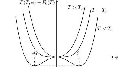
The central idea of Landau theory is that the free energy is an analytic function⁵⁶ of the order parameter ϕ, and as such possesses a Taylor expansion about ϕ=0. Denote with F(T,ϕ) the Landau free energy,⁵⁷ which under the assumption of analyticity can be written

F(T,ϕ)=F0(T)+a2(T)ϕ2+a3(T)ϕ3+a4(T)ϕ4+⋯ ,

(7.76)

where the expansion coefficients a_k are functions of T (and other thermodynamic variables) and F0(T) pertains to the system associated with ϕ=0. In equilibrium free energy is a minimum. The symbol ϕ in F(T,ϕ) is a placeholder for conceivable values of ϕ; the actual values of ϕ representing equilibrium states at temperature T are those that minimize F(T,ϕ). For this reason, F(T,ϕ) is referred to as the Landau free energy functional.⁵⁸ The free energy F(T,ϕ) has a minimum whenever two conditions are met:

⁵³Landau received the 1962 Nobel Prize in Physics for work in condensed matter theory, especially that of liquid helium.

⁵⁴See the review article by Kadanoff et al.[84]

⁵⁵The 2008 Nobel Prize in Physics was awarded to Y. Nambu, M. Kobayashi, and T. Maskawa for discoveries of spontaneous symmetry breaking in subatomic physics.

⁵⁶There are two senses in which the word analytic is used. A formula is said to be analytic when we have a closed-form expression. Another sense in which the term is used, apropos of Landau theory, is that a function f(x) is analytic at x=x0 if it possesses a power-series representation for |x−x0|<r, the interval of convergence of the series. An analytic function has derivatives of all orders, which are themselves analytic at x=x0. See for example [16].

⁵⁷The distinction between Gibbs and Helmholtz energies is dropped at the level of Landau theory; we simply refer to the Landau free energy. It’s assumed that thermodynamic quantities can be found from the Landau free energy through differentiation when evaluated in an equilibrium state.

∂F∂ϕT=0 ∂2F∂ϕ2T≥0 .

(7.77)

There is no term linear in ϕ in Eq. (7.76), which would imply an equilibrium state with ϕ≠0 for T>Tc. The types of terms appearing in Landau functionals reflect the symmetries of the system and the tensor character of the order parameter.⁵⁹ For magnetic systems, the cubic term can be ruled out. The order parameter (magnetization) is a vector that changes sign under time reversal,⁶⁰ yet the free energy must be time-reversal invariant—hence we eliminate the cubic term; a3=0.

For T>Tc, equilibrium is represented by ϕ=0; F(T,ϕ) has a minimum at ϕ=0 if a2>0,a4>0. For T<Tc, the state of the system is represented by ϕ≠0; F(T,ϕ) has a minimum for ϕ≠0 if a2<0,a4>0. (We require a4>0 for stability—as ϕ gets large, so does the free energy.) By continuity, therefore, at T=Tc, a2=0. Figure 7.9 shows F(T,ϕ)−F0(T) for a2>0 ( T≥Tc), a2=0 ( T=Tc), and a2<0 ( T<Tc). We can “build in” the phase transition by taking⁶¹

a2(T)=a0(T)T−Tc ,

(7.78)

Figure 7.9Landau functional F(ϕ) as a function of ϕ for T>Tc, T=Tc, and T<Tc. For T≥Tc, equilibrium is associated with ϕ=0; for T<Tc, the equilibrium state is one of broken symmetry with ϕ=±ϕ0. The dashed line indicates the convex envelope.

where a0(T) is a slowly varying, positive function of T. For magnetic systems,

F(T,ϕ)=F0(T)+a0(T)T−Tcϕ2+a4(T)ϕ4+O(ϕ6) .

(7.79)

Equation (7.79) should be compared with Eq. (7.63) (free energy of the Weiss ferromagnet); they have the same form for small values of the order parameter.⁶² The free energy is a convex function of ϕ (see Section 4.3). The dashed line in Fig. 7.9 is the convex envelope, a line of points at which ∂2F/∂ϕ2=0, connecting the two points at which ∂F/∂ϕ=0.

⁵⁸Just as the Lagrangian L(q,q˙) is a function of all possible coordinates and velocities (q,q˙), where the actual coordinates and velocities are selected through the Euler-Lagrange equation (C.18) to minimize the action, the Landau free energy F(ϕ) is like a Lagrangian in that it satisfies a variational principle to minimize the free energy; see Section 8.6.2.

⁵⁹The order parameter can be a scalar, vector, or tensor depending on the system (see for example de Gennes and Prost[100]), and there are ways of contracting tensors so as to produce invariants reflecting the symmetries of the system (the free energy is a scalar quantity).

⁶⁰Currents would reverse upon a reversal of time, and therefore the magnetic field. Think Amp e` re’s law.

⁶¹One should appreciate the phenomenological character of the Landau theory.

⁶²Equation (7.63) comes from integrating the thermodynamic relation B(M)=(∂F/∂M)T, where B(M) is found from the equation of state in the form of a power series in M, Eq. (7.56), and as such, is known only for the first few terms associated with small values of the order parameter.

7.7.2 Landau critical exponents

7.7.2.1Order parameter exponent, β

For T<Tc, we require F(T,ϕ) to have a minimum at ϕ=ϕ0≠0; from ∂F/∂ϕT,ϕ=ϕ0=0 we find that

ϕ0=±a02a4(Tc−T) . (T<Tc)

(7.80)

Thus, β=12. Compare Eq. (7.80) (from Landau theory) with Eqs. (7.36) or (7.54), the analogous formulas in the van der Waals and Weiss theories. In Section 7.4.1, we referred to β as the “shape of the critical region” exponent; we didn’t have the language of order parameter in place yet.

7.7.2.2Susceptibility exponent, χ

To calculate the susceptibility, we have to turn on a symmetry breaking field, let’s call it f, a generalized force conjugate to the order parameter. (For magnets, we’re talking about the magnetic field.) For this purpose, the Landau free energy is modified:⁶³

F(T,ϕ;f)≡F(T,ϕ)−fϕ=F0(T)+a0(T−Tc)ϕ2+a4ϕ4−fϕ .

(7.81)

Didn’t we say there is no linear term in ϕ? Indeed, f≠0 precludes the possibility of a continuous phase transition: ϕ≠0 for all temperatures. We’re interested in the response of the system to infinitesimal fields. The susceptibility χ associated with order parameter ϕ is defined as

χ≡∂ϕ∂fT,f=0 .

(7.82)

The equilibrium state predicted by the modified free energy is found from the requirement

∂F∂ϕT=0=2a0(T−Tc)ϕ+4a4ϕ3−f .

(7.83)

Equation (7.83) is the equation of state near the critical point. We can calculate χ by differentiating Eq. (7.83) implicitly with respect to f:

∂ϕ∂fT2a0(T−Tc)+12a4ϕ2−1=0⇒χ=12a0(T−Tc)+12a4ϕ2|f=0 .

(7.84)

Because we’re to evaluate Eq. (7.84) for f=0, we can use the known solutions for ϕ in that limit. We have

χ=2a0(T−Tc)−1T>Tc4a0(Tc−T)−1T<Tc .

(7.85)

Thus, γ=1 in Landau theory.

7.7.2.3Critical isotherm exponent, δ

At T=Tc, ϕ→0 as f→0 such that f~ϕδ, implying from Eq. (7.83) with T=Tc,

f=4a4ϕ3 .

(7.86)

Thus, δ=3 in Landau theory.

7.7.2.4 Heat capacity exponent, α

By definition,

CX≡−T∂2F∂T2X .

(7.87)

See Eqs. (P1.5), (P1.6), and (7.62) for examples of C_X obtained from the second partial derivative of a thermodynamic potential with respect to T. Differentiate Eq. (7.81) twice (set f=0) assuming that a0,a4 vary slowly with temperature and can effectively be treated as constants:

∂2F∂T2=∂2F0∂T2+2a0(T−Tc)ϕ∂2ϕ∂T2+∂ϕ∂T2+4a0ϕ∂ϕ∂T+4a4ϕ3∂2ϕ∂T2+12a4ϕ2∂ϕ∂T2 .

Combining with Eq. (7.87), there is a discontinuity at T=Tc:

CX(Tc−)−CX(Tc+)=Tca022a4 ,

(7.88)

where a0,a4 can be functions of the variables implied by X. Thus, we have a discontinuity and not a divergence; α=0 in Landau theory.

7.7.3 Analytic or nonanalytic, that is the question

The critical exponents predicted by Landau theory are not in good agreement with experiment.⁶⁴ Its key assumption, that the free energy function is analytic, is not true at T=Tc: partial derivatives of F do not generally exist at critical points. Phase transitions are associated with points in thermodynamic state space where the free energy is singular. The partition function, however,

Z(N,V,T)=1N!λT3N∫Vdr1⋯∫VdrNexp⁡[−β∑1≤i<j≤Nv(|ri−rj|)]

is an analytic function of T for finiteN,V (the integrand is an analytic function of β and the integral is over a finite domain). For statistical mechanics to have anything to say about phase transitions (at which F=−kTln⁡Z shows singular behavior), we must consider infinite systems, in particular the thermodynamic limit of N,V→∞ with N/V fixed. Up until the 1940s, it was not known whether the “algorithm” of statistical mechanics, the partition function, is sufficient to predict phase transitions. In 1944, L. Onsager⁶⁵ published an exact evaluation of the partition function for the d=2 Ising model (see Section 7.10), showing that a continuous phase transition is indeed obtained in the thermodynamic limit.[102]

The free energy of the two-dimensional Ising model (after the thermodynamic limit has been taken) has the form near the critical point[103, p668]

F(T,M=0)=F(Tc,0)+a(T−Tc)+bT−Tc2ln⁡T−Tc+⋯ , (d=2 Ising)

(7.89)

where a,b are constants. Because of the logarithmic term, F(T,M=0) does not possess a Taylor expansion about T=Tc. The heat capacity derived from Eq. (7.89) has a logarithmic singularity⁶⁶

C≈−2bTln⁡T−Tc+⋯ . (d=2 Ising)

(7.90)

The logarithmic singularity at T=Tc (not a power law) implies α=0 (see Eq. (7.42)). A critical exponent of zero cannot distinguish a discontinuity as in Eq. (7.88) from a logarithmic singularity.

7.7.4 Internal energy in Landau theory

In the van der Waals and Weiss theories, we started with an equation of state (Eqs. (6.32) and (7.49)), and not a Hamiltonian (in essence a dividing line between thermodynamics and statistical mechanics). We found expressions for the free energy in these theories by integrating the equation of state; Eqs. (7.63) and (P7.1). Landau theory starts by positing the form of the free energy in the critical region. Can the internal energy be found if the free energy is known? Consider that

F=U−TS=U+T∂F∂T⇒U=−T2∂(F/T)∂T .

(7.91)

Equation (7.91) is the Gibbs-Helmholtz equation [3, p93]. If we know F, we can find U. Applying Eq. (7.91) to the Landau free energy, Eq. (7.79), we find, near the critical point,

U(T<Tc)=U(T>Tc)−a0Tϕ02 ,

(7.92)

where ϕ₀ is the order parameter, Eq. (7.80). Equation (7.92) should be compared with Eq. (P7.3) (internal energy of the van der Waals gas)—in both cases the energy is reduced in the ordered phase by a term that uniformly couples to all particles of the system, the signature of a mean field theory.

7.8 Mean-field theory: Uncorrelated fluctuations

Landau theory posits a free energy function F(T,ϕ) for small values of the order parameter ϕ, such as in Eq. (7.79). Is there a type of system that, starting from a Hamiltonian,⁶⁷ is found to possess the Landau free energy in the critical region? As we show, Landau theory applies to systems in which the energy of interaction between fluctuations is negligible, in which fluctuations are independent. Consider a lattice model, which for simplicity we take to be the Ising model,

H=−12∑i=1N∑j=1NJijσiσj−b∑i=1Nσi ,

(7.93)

where the factor of 12 prevents overcounting. The Ising Hamiltonian in Eq. (7.93) is more general than that in Eq. (6.68). It’s not restricted to one spatial dimension—it holds in any number of dimensions and it indicates that every spin interacts with every other spin. Usually one takes Jij=0 except when sites i,j are nearest neighbors. A model with interactions of arbitrary range, as in Eq. (7.93), allows us to discuss the molecular field.

Make the substitution σi=σi−〈σ〉+〈σ〉≡〈σ〉+δσi in the two-spin terms in Eq. (7.93):

H=−12∑i=1N∑j=1NJij[(〈σ〉+δσi) (〈σ〉+δσj)]−b∑i=1Nσi=−12∑i=1N∑j=1NJij[〈σ〉2+〈σ〉δσi+〈σ〉δσj+δσiδσj︸ignore]−b∑i=1Mσi≈−12〈σ〉2 ∑i=1N∑j=1NJij−〈σ〉 ∑i=1N∑j=1NJij(σj−〈σ〉)−b ∑i=1Nσi=12〈σ〉2∑i=1N∑j=1NJij−∑i=1N(b+〈σ〉∑j=1NJij)σi .

(7.94)

The mean field approximation ignores couplings between fluctuations (as in Eq. (7.94)). Define q≡∑j=1NJij, the sum of all coupling coefficients connected to site i, which because of translational invariance is independent of i. The value of q depends on the spatial dimension d of the space that the lattice is embedded in. For nearest-neighbor models, q=2J in one dimension, q=4J for the square lattice, and q=6J for the simple cubic lattice. The mean field Hamiltonian is⁶⁸

Hmf≡12Nq〈σ〉2−(b+q〈σ〉)∑i=1Nσi .

(7.95)

Ignoring interactions between fluctuations therefore produces a model (like the Weiss model) in which each spin couples to the external field b and to an effective field q〈σ〉 established by the other spins (the molecular field).⁶⁹ The partition function associated with Eq. (7.95) is easy to evaluate:

Z=e−12βN q〈σ〉2∏i=1N(∑σi=−1Neβ(b+q〈σ〉)σi)=e−12βN q〈σ〉2 (2 cosh [β(b+q〈σ〉)])N .

(7.96)

The free energy per spin is therefore ( F=−βln⁡Z)

1NF=12q〈σ〉2−kT ln (2 cosh [β(b+q〈σ〉)]) .

(7.97)

Equation (7.97)—the mean-field free energy—is not manifestly in the Landau form.⁷⁰ To bring that out, we need to know the critical properties. From 〈σ〉=−(1/N)∂F/∂bT, we find

〈σ〉=tanh⁡β(b+q〈σ〉) ,

(7.98)

the same as Eq. (7.49) (Weiss theory), except that here we have a spin- 12 system.⁷¹ Equation (7.98) predicts⁷² Tc=q/k (see Exercise 7.19). The order parameter in this model is therefore:

〈σ〉=0T≥Tc3TTcTc−TTcT<Tc .

(7.99)

For small 〈σ〉, Eq. (7.97) has the form, for b=0 and expanding⁷³ ln⁡(cosh⁡x),

1NF=−kT ln 2+12k(TcT)(T−Tc) 〈σ〉2+112 kTc (TcT)3〈σ〉4+O(〈σ〉6) ,

(7.100)

which is in the Landau form, Eq. (7.79).

⁶⁸Students sometimes say that the term 12Nq〈σ〉2 in Eq. (7.95) can be dropped because a constant added to a Hamiltonian has no effect on the dynamical behavior of the system. While true in classical mechanics, it’s not the case here—see Exercise 7.17. The “constant” is a function of N,T. Such reasoning is a side effect of calling the Ising Hamiltonian a Hamiltonian, whereas it’s an energy function of spin configurations. Ising spins are not canonical variables.

⁶⁹It should not be construed that mean field theory is “just” a system of spins interacting with a magnetic field (which was covered in Section 5.2). The mean field is determined self-consistently through the equation of state, Eq. (7.98). It’s often said that mean field theory “ignores fluctuations,” which is true at the level of the Hamiltonian where the energy of interaction between fluctuations is ignored, but it’s not the case that fluctuations are absent from mean field theory. The susceptibility in Landau theory diverges at the critical point, just not with the correct exponent.

⁷⁰Mean field theory is more general than Landau theory; it reduces to the latter in the critical region.

⁷¹The Brillouin function B12(x)=tanh⁡x, while the Langevin function L(x)=lim⁡J→∞BJ(x). See Exercise 5.9.

⁷²Up to this point, the value of T_c has been taken as an experimentally determined quantity. The existence of a critical temperature is shown to occur within the models we have set up, with its value taken from experiment. In mean field theory, we have, for the first time, a prediction of T_c in terms of the microscopic energies of the system, kTc=q. The accuracy of that prediction is another matter—see Table 7.2.

⁷³For small x, ln⁡(cosh⁡x)≈12x2−112x4+O(x6).

Mean-field theory predicts continuous phase transitions, even in one dimension, which is unphysical; see Section 7.12. For nearest-neighbor models, q=zJ, where z is the coordination number of the lattice, the number of nearest neighbors it has. For such models, the critical temperature predicted by mean field theory, Tc=zJ/k, would be the same for lattices with the same coordination number. Table 7.2 compares the mean-field critical temperature Tcmf with the critical temperature T_c of the Ising model on various lattices.⁷⁴ The mean field approximation does not accurately account for the effects of dimensionality⁷⁵ for d=1,2,3. Our question has been answered, however: Landau theory applies to systems in which the energy of interaction between spatially separated fluctuations is negligible—noninteracting fluctuations. The message is clear: If we want more accurate predictions of critical phenomena we have to include couplings between fluctuations.

Table 7.2 Mean field critical temperature Tcmf and T_c for the nearest-neighbor Ising model on various lattices. Kc≡J/(kTc). Source: R.J. Creswick, H.A. Farach, and C.P. Poole, *Introduction to Renormalization Group Methods in Physics*.[104, p241]
Lattice	Dimension d	Coordination number z	Tcmf/Tc=zKc
Honeycomb	2	3	1.976
Square	2	4	1.763
Triangular	2	6	1.643
Diamond	3	4	1.479
Simple cubic	3	6	1.330
Body centered cubic	3	8	1.260
Face centered cubic	3	12	1.225

7.9 When is mean field theory exact?

Is there a type of system for which mean field theory is exact, wherein there’s no need to invoke the mean field approximation? That question was answered in Section 7.3.2: The Lebowitz-Penrose theorem shows generally that mean field theory is obtained in models featuring infinite-ranged interactions, in any dimension. In this section, we illustrate how that comes about using the Ising model. We also show that mean field theory becomes exact in systems of spatial dimension d>4.

7.9.1 Weak, long-range interactions

Consider an Ising model,

H=−2JN∑1≤i<j≤Nσiσj ,

(7.101)

where the factor of N−1 keeps the energy extensive (H would scale as N² without it) and the factor of two is for convenience. In contrast to Eq. (7.93), the interaction strength is independent of inter-spin separation; all spins couple with the same strength regardless of separation (it’s not a physical model, yet we learn something). The critical temperature of this model is finite, kTc=q=∑i=1N(2J/N)=N(2J/N)=2J (see Section 7.8). We note the identity for Ising spins:

(∑i=1Nσi)2=∑i=1N∑j=1Nσiσj=∑i=1Nσi2+2∑1≤i<j≤Nσiσj=N+2∑1≤i<j≤Nσiσj .

The Hamiltonian Eq. (7.101) can therefore be rewritten, exactly,

H=J−JN(∑i=1Nσi)2 .

(7.102)

The partition function associated with this Hamiltonian is:

Z=∏i=1N∑σi=−11e−βH=e−K∏i=1N∑σi=−11exp⁡KN(∑i=1Nσi)2 ,

(7.103)

where K≡βJ. Equation (7.103) appears to have presented us with a sum that can’t be evaluated in closed form (in contrast to Eq. (7.96)), were it not for a well chosen identity,

exp⁡(a2)=12π∫−∞∞e−x2/2e2axdx .

(7.104)

Equation (7.104) has a fancy name (even though it follows from completing the square in the argument of the integrand), the Hubbard-Stratonovich transformation,⁷⁶ an integral representation of the exponential of the square of a quantity a that involves the exponential of a term linear in a. The variable x in Eq. (7.104) has no direct physical meaning.

To make use of Eq. (7.104), let a≡(K/N)∑i=1Nσi. Combining Eqs. (7.103) and (7.104),

Z=12πe−K∫−∞∞e−x2/2∏i=1N∑σi=−11exp⁡[(2KN∑i=1Nσi)x]dx=12πe−K∫−∞∞e−x2/2[2cosh⁡(2KNx)]Ndx=2NN2πe−K∫−∞∞e−y2/2cosh⁡2KyNdy≡2NN2πe−K∫−∞∞eNg(y)dy ,

(7.105)

where we’ve changed variables, x=Ny, and where

g(y)=ln⁡e−y2/2cosh⁡2Ky=−y22+ln⁡cosh⁡2Ky .

(7.106)

The final step in Eq. (7.105) sets us up for the method of steepest descent, a method for approximately evaluating integrals of the form ∫−∞∞eNg(y)dy, where N is large and g(x) has a local maximum.[16, p233] The method requires us to find the maximum of g(y). From Eq. (7.106),

g′(y)=−y+2K tanh(2Ky)=0⇒y0=2K tanh(2Ky0)

(7.107)

such that g′(y0)=0. By a method of analysis that should be familiar by now, Eq. (7.107) has a nontrivial solution for K>12 and the trivial solution for K<12, implying kTc=2J. For K≳12, the solution of Eq. (7.107) has the form,

y0~3TTcTc−TTc~−3t , (T→Tc−, t→0−)

(7.108)

virtually the same as Eq. (7.99). We must verify that g(y) has a maximum at y=y0. It’s shown in Exercise 7.20 that g′′(y0)<0 for K>12 and g′′(0)<0 for K<12. It’s straightforward to show that g′′(y0)=2K−1−y02. In the vicinity of y=y0, we have the first few terms of a Taylor series:

g(y)≈g(y0)+(y−y0)g′(y0)−012(y−y0)2 |g″(y0)| .

Therefore,

∫−∞∞eNg(y)dy≈eNg(y0)∫−∞∞e−12Ng′′(y0)(y−y0)2dy=22πNg′′(y0)eNg(y0) .

(7.109)

where we’ve used a Gaussian integral (Appendix B). Combining Eq. (7.109) with Eq. (7.105),

Z=2e−Kg′′(y0)2NeNg(y0) .

(7.110)

The free energy per spin, is, in the thermodynamic limit,

lim⁡N→∞FN=−kTlim⁡N→∞1Nln⁡Z=12kTy2−kTln⁡2 cosh⁡(2Ky) ,

(7.111)

which should be compared with Eq. (7.97) (for b=0). The two formulas agree if we make the correspondence between the order parameter 〈σ〉 and that of the infinite range model, y0↔2K〈σ〉.

7.9.2 The Ginzburg criterion; upper critical dimension

Mean field theory results either from ignoring interactions between fluctuations (Section 7.8) or by having all spins coupled with the same interaction strength⁷⁷ (Section 7.9.1); each is equivalent in its predictions with that of Landau theory in the critical region, which, as we’ve noted, are not in good agreement with experiment. Away from the critical region, however, mean field theory does an adequate job in treating the thermodynamic properties of interacting systems.⁷⁸ Is there a physical argument why Landau theory fails in the critical region?

In 1961, V.L. Ginzburg offered a criterion,⁷⁹ the Ginzburg criterion, for the conditions under which the approximation of uncorrelated fluctuations is justified.[105] Consider the following ratio,

R≡∫ξdg(r)ddr∫ξdϕ2(r)ddr ,

(7.112)

where g(r)≡〈δϕ(0)δϕ(r)〉 denotes the two-spin correlation function, and ϕ(r) is the order parameter.⁸⁰ The numerator in Eq. (7.112) is an average over a d-dimensional region whose linear dimension is of order ξ; it’s important not to average over a region larger than ξ^d, otherwise we have uncorrelated fluctuations. The denominator is a measure of the square of the order parameter, ϕ², averaged over the same volume, ξ^d. The ratio R characterizes the strength of correlated fluctuations in a d-dimensional ball of radius ξ, 〈(δϕ)2〉ξ, relative to the square of the order parameter, 〈ϕ2〉ξ averaged over the same hypervolume. If R≪1 (Ginzburg criterion), Landau theory applies; if not, it fails in the critical region.⁸¹

In the critical region, the denominator in Eq. (7.112) can be approximated ∫ξdϕ2(r)ddr~ξdt2β~ξd−(2β/ν), where we’ve used ϕ~tβ along with ξ~t−ν, where t is the reduced temperature. Similarly, for the numerator ∫ξdg(r)ddr~χ~t−γ~ξγ/ν. The ratio R in Eq. (7.112) therefore scales with ξ as

R~ξ−d+(γ+2β)/ν .

(7.113)

For d>(γ+2β)/ν, R→0 as ξ→∞, and Landau theory is valid. Using the classical exponents, (γ+2β)/ν=4; Landau theory gives a correct description of critical phenomena in systems for which d>4. For d<4, the Ginzburg criterion is not satisfied and Landau theory does not apply in the critical region. The case of d=4 is marginal and requires more analysis; Landau theory is not quite correct in this case. The special dimension d=4 is referred to as the upper critical dimension.

7.10 The two-dimensional Ising model

The two-dimensional Ising model occupies an esteemed place in statistical mechanics as one of the few exactly solvable, nontrivial models of phase transitions; no textbook on the subject can be complete without it. Onsager’s 1944 derivation is a mathematical tour de force, of which the search for simplifications has become a field of research, but even the simplifications are rather complicated. Books have been written on the two-dimensional Ising model [107, 108]. We outline the method of solution and then examine the thermodynamic properties of this model.

7.10.1 Partition function, free energy, internal energy, and specific heat

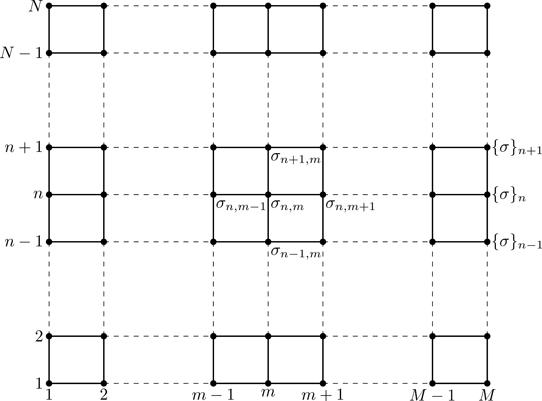
Figure 7.10 shows an N×M array of Ising spins σn,m in the nth row and mth column, 1≤n≤N, 1≤m≤M. The nearest-neighbor Hamiltonian can be written⁸²

H=−J∑n=1N∑m=1M−1σn,mσn,m+1︸intra-rowcouplings −J∑n=1N−1∑m=1Mσn,mσn+1,m︸inter-rowcouplings .

(7.114)

Figure 7.10N×M array of Ising spins σn,m. All spins in row p are denoted {σ}p≡{σp,m}|m=1M.

Periodic boundary conditions are assumed (the lattice is on the surface of a torus), and thus the summation limits in Eq. (7.114), N−1, M−1 can be replaced with N,M. Give names to the terms containing intra and inter-row couplings,⁸³

V1({σ}n)≡∑m=1Mσn,mσn,m+1 V2({σ}n, {σ}n+1)≡∑m=1Mσn,mσn+1,m ,

where {σ}n≡σn,1,⋯,σn,M denotes all spins in the nth row (see Fig. 7.10). We must evaluate the sum

ZN,M(K)=∑{σ}1,⋯,{σ}Nexp [K(∑n=1NV1({σ}n)+V2({σ}n,{σ}n+1))]≡∑{σ}1,⋯,{σ}NT{σ}1,{σ}2T{σ}2,{σ}3⋯T{σ}N−1,{σ}NT{σ}N,{σ}1=Tr(T)N ,

(7.115)

where K≡βJ and we’ve introduced the transfer matrix T (see Section 6.5), with elements

T{σ},{σ}′=eKV1({σ})eKV2({σ},{σ}′) .

T{σ},{σ}′ is a 2M×2M matrix (which is why we can’t write down an explicit matrix form); it operates in a space of 2^M spin configurations. It can be put in symmetric form (and thus it has real eigenvalues):

T{σ},{σ}′=e12KV1({σ})eKV2({σ},{σ}′)e12KV1({σ}′) .

The trace in Eq. (7.115) is a sum over the eigenvalues of T, λ_k, 1≤k≤2M (see Section 6.5):

ZN,M(K)=TrTN=∑k=12MλkN .

Assume we can order the eigenvalues with λ1≥λ2≥⋯≥λ2M, in which case

ZN,M=λ1N∑k=12Mλkλ1N .

(7.116)

The free energy per spin, ψ, is, in the thermodynamic limit, using Eq. (7.116),

−βψ≡−βlim⁡M,N→∞FMN=lim⁡M,N→∞1MNln⁡ZN,M=lim⁡M→∞1Mln⁡λ1(M) ,

(7.117)

where we’ve written λ1(M) in Eq. (7.117) to indicate that it’s the largest eigenvalue of the 2M×2M transfer matrix. “All” we have to do is find the largest eigenvalue λ1(M) in the limit M→∞ !

Through a masterful piece of mathematical analysis, Onsager did just that. He showed, for large M, that

λ1(M)(K)=(2 sinh 2K)M/2 e12(γ1(K)+γ3(K)+⋯+γ2M−1(K)) ,

(7.118)

where

cosh⁡γk(K)≡cosh⁡2Kcoth⁡2K−cos⁡(πkM) .

(7.119)

A derivation of Eq. (7.118) is given in Thompson.[109, Appendix D] Combining Eqs. (7.118) and (7.117),

−βψ=12ln⁡(2sinh⁡2K)+lim⁡M→∞(12M∑k=0M−1γ2k+1) .

(7.120)

As M→∞, the sum in Eq. (7.120) approaches an integral (let πk/M≈θ):

−βψ=12ln(2 sinh 2K)+12π∫0πcosh−1 [cosh 2K coth 2K−cosθ] dθ ,

(7.121)

where cosh⁡−1 comes from Eq. (7.119) for γ_k. The integral in Eq. (7.121) would appear hopeless, were it not for a well chosen identity.⁸⁴ An integral representation of inverse hyperbolic cosine is:⁸⁵

cosh⁡−1|z|=1π∫0πln⁡[2(z−cos⁡ϕ)]dϕ .

(7.122)

Combine Eq. (7.122) with Eq. (7.121), and we have an expression for the free energy per spin,

−βψ=12ln (2 sinh 2K)+12π2∫0π∫0πln [2 (cosh 2K coth 2K−cosθ−cosϕ)] dθdϕ.

(7.123)

It’s a simple step to put all terms in Eq. (7.123) associated with K “inside” the integral:

−βψ=ln2+12π2∫0π∫0πln [cosh2 2K−sinh 2K (cosθ+cosϕ)] dθdϕ .

(7.124)

Examining Eq. (7.124) (which holds for any T), we find that the integrand has a logarithmic singularity at the origin ( θ,ϕ→0) when the temperature has a special value T_c such that cosh⁡22Kc=2sinh⁡2Kc ( Kc≡J/(kTc)), which we identify as the critical temperature. There is a unique solution of cosh⁡22Kc=2sinh⁡2Kc,

sinh⁡2Kc=1 ,

(7.125)

implying Kc≈0.4407. The largest eigenvalue of a finite transfer matrix is an analytic function of K (see Section 6.5.3). Given that the free energy is related to the largest eigenvalue, and that phase transitions are associated with singularities in the free energy (Section 7.7.3), we conclude there is no phase transition in one dimension for T>0 (see Section 7.12). For the two-dimensional Ising model, the largest eigenvalue of the transfer matrix becomes singular in the thermodynamic limit⁸⁶ for K=Kc.

⁸⁴See the same remark near Eq. (7.104).

⁸⁵Equation (7.122) is not a standard identity. The inverse hyperbolic cosine has a logarithmic representation, cosh⁡−1|z|=ln⁡[z+z2−1],[50, p87] the same as the value of the integral in Eq. (7.122). Because that integral shows up again in the Onsager solution, we note that ∫0πln⁡a+bcos⁡xdx=πln⁡12a+a2−b2, a>|b|>0. The integrand is periodic with period 2π, so the limit of integration can be extended to 2π, doubling the value of the integral.

⁸⁶The finite sum in Eq. (7.118) specifies an analytic function λ1(M)(K) for all K and finite M; the resulting integral in Eq. (7.124) for M→∞ has a singularity when cosh⁡22K=2sinh⁡2K. In taking limits, mathematical properties can be lost. Consider the Taylor series for ex. Set x=1. For any finite number of terms in the series, the result specifies a rational number. Only in the limit of an infinite number of terms does one obtain the irrational number, e. I thank Professor Chris Frenzen for that observation.

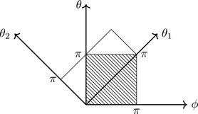
Equation (7.124) can be simplified through the trigonometric identity cosθ+cosθ=2 cos (12(θ+ϕ)) cos (12(θ−ϕ)), which suggests a change of variables. Let

θ1≡12(θ+ϕ) θ2≡θ−ϕ .

(7.126)

No factor of 12 is included in θ₂ so that the Jacobian of the transformation is unity (see Section C.9):

dθ1dθ2=∂(θ1,θ2)∂(ϕ,θ)dϕdθ=dϕdθ .

The geometry of the coordinate transformation Eq. (7.126) is shown in Fig. 7.11. You should verify that θ1=0,θ2=π corresponds to θ=π/2,ϕ=−π/2, and θ1=π,θ2=0 corresponds to ϕ,θ=π. The transformation is not a rigid rotation, although it is area preserving (Exercise 7.25). Making the substitutions, we have from Eq. (7.124),

−βψ=ln2+12π2∫0πdθ1∫0πdθ2ln (cosh2 2K−2 sinh 2K cosθ1 cos(θ2/2))=ln(2 cosh 2K)+1π2∫0πdθ1∫0πdωln (1−κ(K) cosθ1cosω) ,

(7.127)

Figure 7.11Geometry of the coordinate transformation in Eq. (7.126).

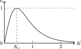
where ω≡θ2/2 and

κ(K)≡2sinh⁡2Kcosh⁡22K .

(7.128)

Figure 7.12 shows a plot of κ(K); it equals unity at K=Kc. It’s worth stating that κ(K) is an analytic function. Because |κcos⁡ω|≤1 (Exercise 7.21), we can integrate over θ₁ in Eq. (7.127):

−βψ=ln (2 cosh 2K)+1π∫0π/2ln (12(1+1−κ2 cos2 ω)) dω .

(7.129)

The value of the integral in Eq. (7.129) is unchanged⁸⁷ if cos⁡2ω is replaced with sin⁡2ω, which is more convenient. Thus, we have our final expression for the free energy of the d=2 Ising model,

−βψ=ln⁡(2 cosh⁡2K)+1π∫0π/2ln⁡(12(1+1−κ2sin⁡2ω))dω .

(7.130)

Combining Eq. (7.130) with Eq. (7.91) (Gibbs-Helmholtz equation), we have the internal energy per spin (specific energy), u, which, after a few steps has the form⁸⁸

u=−J∂∂K(−βψ)=−J coth 2K[1+2π(2 tanh2 2K−1)F(κ)] ,

(7.131)

where F is the complete elliptic integral function of the first kind,[50, p590]

F(y)≡∫0π/2dω1−y2sin⁡2ω , (0≤y<1)

(7.132)

the values of which are tabulated. We’ll also require the complete elliptic integral function of the second kind,

E(y)≡∫0π/21−y2sin⁡2ωdω , (0≤y≤1)

(7.133)

which shows up through the derivative of F(y) (see Exercise 7.23). E(y) has no singularities.

The specific heat c is obtained from one more derivative:

c=∂u∂T=−KT∂∂Ku=4πk (K coth 2K)2[F(κ)−(1−tanh2 2K) [π2+(2 tanh2 2K−1) F(κ)]].

(7.134)

The elliptic integral F(y) diverges logarithmically as y→1−, which we see from the asymptotic result[110, p905]

F(y)~y→1−ln⁡(41−y2) .

(7.135)

The heat capacity therefore has a logarithmic singularity at T=Tc, as we see in Eq. (7.90), implying α=0 for the two-dimensional Ising model.

7.10.2 Spontaneous magnetization and correlation length

The Onsager solution is a landmark achievement in theoretical physics, an exact evaluation of the partition function of interacting degrees of freedom in a two-dimensional system, from which we obtain the free energy, internal energy, and specific heat. We identified T_c as the temperature at which the free energy becomes singular ( κ=1). A more physical way of demonstrating the existence of a phase transition would be to calculate the order parameter. The first published derivation of the spontaneous magnetization appears to be that of C.N. Yang,⁸⁹ who showed[111]

〈σ〉=0T>Tc1−1sinh⁡42K1/8T≤Tc .

(7.136)

Clearly the temperature at which 〈σ〉→0 is sinh⁡2Kc=1, the same as Eq. (7.125). We infer from Eq. (7.136) that the order parameter critical exponent β=18, our first non-classical exponent. The small ( ≪1) value of β implies a rapid rise in magnetization for T≲Tc, as we see in Fig. 7.13. Yang’s derivation was later simplified,[112] yet even the simplification is rather complicated.

Figure 7.13Spontaneous magnetization in the two-dimensional Ising model; T1=0.9Tc.

In the one-dimensional Ising model, we found that the correlation length ξ is determined by the largest and second-largest eigenvalues of the transfer matrix (see Eq. (6.101)), with the result ξ(K)=−a/ln⁡(tanh⁡K), where a is the lattice constant. The same holds in the two-dimensional Ising model, with the result[108, Chapter 7]

ξ(K)=−2aln⁡sinh⁡22KT>Tc (K<Kc)aln⁡sinh⁡22KT<Tc (K>Kc) .

(7.137)

For K<Kc ( >Kc), sinh⁡22K<1 ( >1), which is useful in understanding ξ(K) as sinh⁡22K passes through the critical value sinh⁡22Kc=1. In either case, ξ→∞ for K→Kc, such that

ξ~T−Tc−1 ,

(7.138)

and thus ν=1 in the two-dimensional Ising model. Note that ξ(K)→K→00 and ξ(K)→K→∞0.

We now have four of the six critical exponents, α,β,ν,η, where η=14 (Section 7.6). Each is distinct from the predictions of Landau theory. The heat capacity exponent α=0 is seemingly common to both, but Landau theory predicts a discontinuity in specific heat rather than a logarithmic singularity. The remaining two exponents γ,δ will follow with a little more theoretical development (Section 7.11), but we can just state their values here (for the d=2 Ising model) γ=74 and δ=15.

7.11 Critical exponent inequalities

Critical exponents are not independent, which is not surprising given all the thermodynamic interrelations among state variables. We saw in Section 7.4 that γ=2β in the van der Waals model and γ=2ν in Ornstein-Zernike theory (Section 7.6), relations that hold in those particular theories, but which do not apply in general. Finding general relations among critical exponents should start with thermodynamics. As we now show, thermodynamics provides inequalities, but not equalities, among critical exponents that might otherwise reduce the number of independent exponents. Before getting started, we note an inequality among functions that implies an inequality among exponents. Suppose two functions f(x),g(x) are such that f(x)≤g(x) for x≥0, and that f(x)~xψ and g(x)~xϕ as x→0+. Then, ψ≥ϕ. See Exercise 7.26.

Equation (1.51) implies an inequality on the heat capacity of magnetic systems,

CB=0≥Tχ∂M∂TB=02 .

(7.139)

Because CB=0~|T−Tc|−α (Eq. (7.66)), χ~|T−Tc|−γ (Eq. (7.60)), and M~|T−Tc|β (Eq. (7.54)), inequality (7.139) immediately implies Rushbrooke’s inequality,[113]

α+2β+γ≥2 .

(7.140)

Because it follows from thermodynamics, it applies to all systems.⁹⁰ For the d=2 Ising model it implies γ≥74. It’s been shown rigorously that γ=74 for the two-dimensional Ising model [114], and thus Rushbrooke’s inequality is satisfied as an equality among the exponents of the d=2 Ising model. We also have the same equality among classical exponents: α+2β+γ=2.

Numerous inequalities among critical exponents have been derived.⁹¹ We prove one more, Griffiths inequality,[115]

α+β(1+δ)≥2 .

(7.141)

To show this, we note for magnetic systems⁹² that M, T are independent variables of the free energy, F(T,M). Equation (7.61), B=∂F/∂MT, as applied to the coexistence region (which is associated with B=0), implies

(∂F∂M)T=0 , (T≤Tc, 0≤M≤M0(T))

where we use M0(T) to denote the spontaneous magnetization at temperature T (such as shown in Fig. 7.13). The free energy in the coexistence region is therefore independent of M:

F(T,M)=F(T,0) . T≤Tc,0≤M≤M0(T)

(7.142)

It may help to refer to Fig. 7.9, where F is independent of the order parameter along the convex envelope. Entropy is also independent of M in the coexistence region. From the Maxwell relation ∂S/∂MT=−∂B/∂TM (Exercise 1.15), we conclude, because B=0, that

S(T,M)=S(T,0) . T≤Tc,0≤M≤M0(T)

(7.143)

F(T,M) is a concave function⁹³ of T for fixed M. The tangent to a concave function always lies above the curve (see Fig. 4.2), implying the following inequalities derived from the slope F^′ evaluated at a lower temperature T2<T1≤Tc, and F^′ evaluated at a higher temperature, T1>T2:

F(T1,M)≤F(T2,M)+(T1−T2)F′(T2,M)=F(T2,M)−(T1−T2)S(T2,M)F(T2,M)≤F(T1,M)−(T1−T2)F′(T1,M)=F(T1,M)+(T1−T2)S(T1,M) ,

(7.144)

where F′≡∂F/∂TM=−S(T,M), Eq. (7.61). With T1=Tc and T2≡T, and using Eqs. (7.142) and (7.143), the inequalities in (7.144) imply the inequality

F(Tc,M)−F(Tc,0)≤Tc−TS(Tc,0)−S(T,0) .

(7.145)

Note that for M=0 and T=Tc, inequality (7.145) reduces to 0≤0, and students sometimes cry foul—it’s a tautology. We’re interested in how the two sides of the inequality vanish in the limit that the critical point is approached. As M→0 and T→Tc−, inequality (7.145) has the structure

M∂F∂M~MF(Tc,M)−F(Tc,0)M≤Tc−T2S(Tc,0)−S(T,0)Tc−T~Tc−T2∂S∂T .

Using Eqs. (7.61) and (7.62), and that B~Mδ~|T−Tc|βδ and C~|T−Tc|−α, inequality (7.145) implies MB~Mδ+1~T−Tcβ(δ+1)≲T−Tc2−α. We must have therefore that β(δ+1)≥2−α, which is Griffiths inequality, (7.141). For the d=2 Ising model it implies δ≥15. It’s found numerically that δ=15.00±0.08,[103, p694] from which we conclude that δ=15. For the classical exponents, Griffiths inequality is an equality, α+β(δ+1)=2.

Other inequalities among critical exponents have been derived, but none are as general as the Rushbrooke and Griffiths inequalities which follow from thermodynamics.⁹⁴ Under plausible assumptions, additional inequalities have been derived (and this list is not exhaustive):

γ≥β(δ−1) (Griffiths)2−ην≥γ (Fisher)dδ−1δ+1≥2−η . (Buckingham-Gunton)

(7.146)

These inequalities are satisfied as equalities for the critical exponents of the d=2 Ising model; the last inequality fails for classical exponents if d<4. Table 7.3 shows the values of critical exponents, experimental and theoretical. Exponents for the d=3 Ising model are obtained from numerical investigations and are known only approximately.

Table 7.3 Critical exponents. Source: L.E. Reichl, *A Modern Course in Statistical Physics* [117].
Exponent	Experimental value	d=2 Ising	d=3 Ising	Mean field theory
α	0–0.2	0 (logarithmic)	0.110	0 (discontinuity)
β	0.3–0.4	1/8	0.326	1/2
γ	1.2–1.4	7/4	1.237	1
δ	4–5	15	4.790	3
ν	0.6–0.7	1	0.623	1/2
η	0.1	1/4	0.036	0

7.12 The impossibility of phases in one dimension

We noted in Section 7.10 that phase transitions do not occur in one-dimensional systems. We based that conclusion on an analysis of the largest eigenvalue of the transfer matrix for the d=1 Ising model, which by Perron’s theorem is an analytic function of K (and phase transitions are associated with singularities in the free energy function). Perron’s theorem does not apply to infinite matrices, as in the two-dimensional Ising model, where the largest eigenvalue is not an entire function,⁹⁵ and we have a phase transition in two dimensions. One could object that the Ising model is too specialized to draw conclusions about phase transitions in all one-dimensional systems. The Mermin-Wagner-Hohenberg theorem [118, 119] states that spontaneous ordering by means of continuous symmetry breaking⁹⁶ is precluded in models with short-range interactions in dimensions d≤2. The requirement of continuous symmetry breaking is essential—the two-dimensional Ising model in zero magnetic field (discrete symmetry) possesses a spontaneous magnetization. In either case (continuous or discrete symmetries), phase transitions in one dimension are precluded.

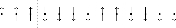
It would be nice if a physical argument could be given illustrating the point. Landau and Lifshitz, on the final page of Statistical Physics [99], present such an argument that we adapt for Ising spins.⁹⁷ Figure 7.14 shows a one-dimensional array of Ising spins consisting of domains of aligned spins separated by interfaces, “domain walls” (dashed lines).⁹⁸ We can consider domains phases, call them A and B or up and down. The question is, is there a finite temperature for which the system consists entirely of one phase, i.e., can there be a phase with long-range order?

Figure 7.14One-dimensional domains of Ising spins, separated by domain walls (dashed lines).

Assume N Ising spins in one dimension, as in Fig. 7.14, coupled through near-neighbor interactions, and let there be m domain walls. The energy of the system is (show this)

U=−J(N−1)+2mJ .

(7.147)

It requires energy 2J to create a domain wall. There are N−1m ways of arranging m domain walls within the system of N spins, and thus the entropy of the collection of domain walls is, for N large,

1kS=ln⁡N−1m~N→∞ln⁡Nmm!=mln⁡Nem ,

(7.148)

where we’ve used Eq. (3.44) and Stirling’s approximation. The free energy is therefore

F=−J(N−1)+2mJ+kTmln⁡mNe .

(7.149)

Free energy is a minimum in equilibrium. From Eq. (7.149),

∂F∂m=2J+kTln⁡mN .

(7.150)

Setting ∂F/∂m=0, the average number of domain walls in thermal equilibrium is

m¯=Nexp⁡(−2J/kT) .

(7.151)

There is no temperature for which m¯=0; entropy wins—an ordered phase in one dimension cannot exist. For the one-dimensional Ising model, ξ(K)~12e2K for K≫1 (Eq. (P6.1)), and hence,

m¯~T→0N2ξ .

(7.152)

As T→0, ξ→∞ implying that m¯→0 in the limit. In one dimension, T=0 is a critical temperature, but there is no “low temperature” phase.⁹⁹

Summary

This chapter introduced phase transitions and critical phenomena, setting the stage for Chapter 8.

Phases are spatially homogeneous, macroscopic systems in thermodynamic equilibrium. Substances exist in different phases depending on the values of state variables. Phases coexist in physical contact at coexistence curves and triple points. The chemical potential of substances in coexisting phases has the same value in each of the coexisting phases. Every PVT system has a critical point where the liquid-vapor coexistence curve ends, where the distinction between liquid and gas disappears. Magnets have critical points as well. The behaviors of systems near critical points are referred to as critical phenomena.
The Gibbs phase rule, Eq. (7.13), specifies the number of intensive variables that can be independently varied without disturbing the number of coexisting phases.
The latent heat L is the energy released or absorbed in phase transitions. Phase transitions are classified according to whether L≠0 —first-order phase transitions—and those for which L=0, continuous phase transitions. For historical reasons, continuous phase transitions are referred to as second-order phase transitions. At first-order phase transitions, there is a change in specific entropy, Δs=L/T. At continuous transitions, Δs=0.
We discussed the liquid-gas phase transition using the van der Waals equation of state, from which we discovered the law of corresponding states, that systems in corresponding states behave the same. Corresponding states are specified by reduced state variables—state variables expressed in units of their critical values, Eq. (7.22). Substances obey the law of corresponding states even if they’re not well described by the van der Waals model; see Fig. 7.3.
The Maxwell construction is a rule by which the coexistence region can be located in a P–v diagram, that the area under the curve of sub-critical isotherms (obtained from the equation of state) be the same as the area under the flat isotherms of coexisting liquid and gas phases. The van der Waals equation of state (motivated phenomenologically, see Section 6.2) and the Maxwell construction occur rigorously in theories featuring weak, long-range interactions (Lebowitz-Penrose theorem), a class of theories known as mean field theory. Besides long-range interactions, mean field theories result when the energy of interaction between fluctuations is ignored—fluctuations are independent and uncorrelated in mean field theories.
The prototype mean field theory is the Weiss molecular field theory of ferromagnetism. It asserts that the aligned dipole moments in the magnetized state contribute to an internal magnetic field, the molecular field. By postulating a proportionality between the molecular field and the magnetization, one arrives at a theory with a nonlinear equation of state, Eq. (7.49), a self-consistent theory where spins respond to the same field they generate. The molecular field is a proxy for the ordering of spins that’s otherwise achieved through inter-spin interactions. Statistical mechanics is particularly simple for mean field theories, while the statistical mechanics of interacting degrees of freedom is not so simple, as we’ve seen.
The order parameter ϕ is a quantity that’s zero for T≥Tc, nonzero for T<Tc, and vanishes smoothly as T→Tc−. The vanishing of ϕ as T→Tc is characterized in terms of an exponent, β, such that ϕ~|T−Tc|β, one of several exponents by which critical phenomena are described. The critical isotherm exponent δ characterizes how the field f conjugate to ϕ behaves in the critical region, with f~ϕδ as ϕ→0 and T=Tc. Other quantities diverge as T→Tc, with each divergence characterized by its own exponent. As T→Tc, the heat capacity C~|T−Tc|−α; for the compressibility (or susceptibility χ) with f=0, βT~|T−Tc|−γ; for the correlation length, ξ~|T−Tc|−ν; for the static structure factor S(q,T), which for T=Tc diverges as S(q,T=Tc)~q−(2−η) as q→0. Critical exponents can be measured and calculated from theory. In standard statistical mechanics, there are six critical exponents: α,β,γ,δ,ν,η.

⁹⁹There are exceptional systems characterized by negative absolute temperature, but negative absolute temperature does not imply a temperature colder than zero. Negative temperatures are hotter than all positive temperatures.[3, p163]
Landau theory describes phase transitions in terms of a model free energy function, F(ϕ,T), Eq. (7.79). The graph of F(ϕ,T), shown in Fig. 7.9, is one of the more widely known diagrams in physics. One sees that for T≥Tc, the minimum (equilibrium state) occurs at ϕ=0; for T<Tc, the equilibrium state is one of broken symmetry with ϕ=±ϕ0. Landau theory is a mean field theory. The critical exponents predicted by mean field theories are all the same, the classical exponents: α=0, β=12, γ=1, δ=3, ν=12, η=0.
The classical exponents are not in good agreement with experiment; see Table 7.3. The key assumption of Landau theory is that the free energy function is analytic, which is not correct—partial derivatives of F generally do not exist at the critical point. Phase transitions are associated with points in thermodynamic state space where the free energy function is singular. For finite N and V, the partition function is an analytic function of its arguments; to describe phase transitions, the thermodynamic limit must be taken. Landau theory does an adequate job in treating the thermodynamics of interacting systems away from the critical region. From the Ginzburg criterion, Landau theory applies in the critical region of systems of dimension d>4. We presented the Landau-Lifshitz argument on the impossibility of the existence of long-range order for d=1.
We outlined the Onsager solution of the two-dimensional Ising model in zero magnetic field, which requires that one find the largest eigenvalue of the 2M×2M transfer matrix in the limit M→∞. Starting from Onsager’s formula for the largest eigenvalue, Eq. (7.118), one can see how the free energy develops a singularity in the thermodynamic limit. Exact expressions can be found for the partition function, free energy, internal energy, and heat capacity, which displays a logarithmic divergence at T=Tc, α=0. The theory predicts the critical temperature as that at which the free energy is singular, Kc=0.4407. From Eq. (7.136) for the spontaneous magnetization we infer the non-classical critical exponent β=18.
Critical exponents are not independent of each other. Thermodynamics provides relations among critical exponents in the form of inequalities, such as the Rushbrooke and Griffiths inequalities. Explaining why these inequalities are satisfied as equalities is the starting point of the next chapter.

EXERCISES

7.1An approximate solution of the Clausius-Clapeyron equation can be derived if we assume that: 1) the latent heat L is a constant; 2) vgas≫vliquid, so that Δv≈vgas; 3) the gas is ideal. With these assumptions, show that the coexistence curve has the form P=P0e−L/(kT).
7.2Referring to Fig. 5.14, what is the order in the Ehrenfest classification scheme of the Bose-Einstein condensation?
7.3We argued that V/N≈b is a solution of Eq. (7.18) for small V/N. In what regime would such a guess be correct? Write V/N=b(1+δ), where δ is dimensionless and presumed small, δ≪1. Show at lowest order that δ=kT/(Pb+a/b). Our guess is correct for temperatures such that kT≪(Pb,a/b).

7.4 Show for low temperatures, kT≪Pb, there is only one real root of Eq. (7.18), together with a pair of unphysical, complex conjugate roots. Hint: Look up the formula for the roots of cubic equations (such as in [50, p17]).
7.5The van der Waals model predicts the critical parameters vc,Pc,Tc reasonably well. A gas for which the constants (a,b) are known, as well as the critical parameters is argon (there are many others). For argon, a=1.355 bar L 2/ mol² and b=0.0320 L/mol.[57, p6-33] To convert to SI units, 1 bar L 2/mol2=0.1 Pa m 6/ mol² and 1 L /mol=10−3 m 3/ mol. Use Eq. (7.21) to calculate vc,Pc,Tc and compare with the experimental results Tc=150.87 K, Pc=4.898 MPa, and vc=75 cm³ mol^-1 (see [57, p6-37]). Note that you have to convert from moles to particle number (Avogadro’s number) to find T_c.
7.6Derive the law of corresponding states, Eq. (7.23).
7.7Show that for liquid-gas phase coexistence, the mole fractions in the gas and liquid phases are given by the expressions

xg=vd−vlvg−vl xl=vg−vdvg−vl .

Hint: Use the lever rule, Eq. (7.25).
7.8Thermodynamic properties of the van der Waals gas.
1. Derive the Helmholtz energy, which can be found by integrating the equation of state. Show, from Eq. (4.58), P=−∂F/∂VT,N, that, using Eq. (6.32),
  
  F(T,V,N)=−∫PdV+ϕ(T,N)=−NkTln⁡(V−Nb)−aN2V+ϕ(T,N) ,
  
  where ϕ(T,N), the integration “constant,” is a function of T,N. We can determine ϕ(T,N) by requiring that for a=b=0, we recover the Helmholtz energy of the ideal gas. Show, from −βF=ln⁡Z, Eq. (4.57), that using Eq. (5.1) for Z and the Stirling approximation, we have for the ideal gas F=−NkT1+ln⁡V/(NλT3), implying ϕ(T,N)=NkTln⁡(NλT3)−1, and therefore
  
  F(T,V,N)=−NkTln⁡V−NbNλT3+1−aN2V .
  
  (P7.1)
2. Use the other two expressions in Eq. (4.58) to find the chemical potential and entropy:
  
  μ=−kTln⁡V−NbNλT3+NbkTV−Nb−2aNVS=Nk52+ln⁡V−NbNλT3 .
  
  (P7.2)
  
  The entropy of the van der Waals gas is the same as the ideal gas, except for the excluded volume. Note that the excluded volume Nb (which can be considered a repulsive interaction) makes a positive contribution to the chemical potential, whereas the attractive part, characterized by the parameter a, works to decrease μ. See the remarks on the sign of the chemical potential in Section 1.6.
3. Find the internal energy. Hint: U=F+TS.
  
  U=32NkT−aN2V .
  
  (P7.3)
  
  The energy per particle U/N is modified from its value for the ideal gas (all kinetic energy) to include a contribution from the potential energy of interactions, simply proportional to the average density, −an.
4. Show that the heat capacity C_V of the van der Waals gas is the same as for the ideal gas. Hint: The parameter a is independent of temperature. You could make use of Eq. (P1.7) to show that C_V for the van der Waals model has no volume dependence.
5. From the thermodynamic identity Eq. (1.42),
  
  CP=CV−T∂P∂VT∂V∂TP2 ,
  
  show for the van der Waals gas that,
  
  CP−CVNk=11−2a(v−b)2v3kT .
  
  (P7.4)
7.9Show that the Helmholtz energy of the van der Waals gas, an expression for which is given in Eq. (P7.1), can be written in terms of reduced variables

−FNkT=ln⁡(3v¯−1)T¯3/2+1+ln⁡bλTc3+98T¯v¯ .

(P7.5)

Show from Eq. (P7.5) that Pv/(kT) is a universal function. Hint: P=kT∂(−F/NkT)/∂vT,N.
7.10Guided exercise to derive Eq. (7.32).
1. The specific energy u is a function of specific volume and temperature, u=u(v,T). To see this, assume that U=U(T,V,N). You should convince yourself of this—U is “naturally” a function of (S,V,N) (see Eq. (1.21)), but we can take S as a function of (T,V) (show that dS=(CV/T)dT+(α/βT)dV), and thus, invoking the thermodynamic limit, U=Nf(v,T) and hence u=u(v,T).
2. Referring to Eq. (7.31), for u=u(v,T), show from Eq. (1.32) that
  
  ∂u∂Tcoex=∂u∂Tv+∂u∂vT∂v∂Tcoex=cv+∂u∂vT∂v∂Tcoex .
  
  (P7.6)
3. Use Eq. (1.41) to show that
  
  ∂u∂vT,N=T∂P∂TV,N−P .
  
  (P7.7)
4. We require Δu≡ug−ul. Use Eq. (7.15) to show that the Clausius-Clapeyron equation can be written
  
  dPdTcoex=ΔhTΔv=1TΔvΔu+PΔv=ΔuTΔv+PT ,
  
  implying that
  
  Δu=TdPdTcoex−PΔv .
  
  (P7.8)
5. Differentiate the lever rule, Eq. (7.25), to show that
  
  (vg−vl)∂xl∂Tcoex=xg∂vg∂Tcoex+xl∂vl∂Tcoex .
  
  (P7.9)
  
  Show that Eq. (P7.9) is symmetric under the interchange of labels, g↔l.
6. Show from Eq. (1.32) that for Pcoex=Pcoex(T,v),
  
  dPdTcoex=∂P∂Tv+∂P∂vT∂v∂Tcoex .
  
  (P7.10)
  
  The coexistence curve P_coex is a clearly a function of T (see Fig. 7.1), but it’s also a function of v: The coexistence curve is the projection onto the P–T plane of the coexistence region in the P–v plane.
7. Show that by combining Eqs. (P7.6) through (P7.10), one arrives at Eq. (7.32) starting from Eq. (7.31).
7.11Derive Eq. (7.34), the van der Waals equation of state in the vicinity of the critical point, by substituting Eq. (7.33) into Eq. (7.23) and keeping track of small quantities. Hint: For x≪1, (1+x)−1≈1−x+x2−x3+⋯.
7.12Derive Eq. (7.43), the form of Eq. (P7.4) when expressed in terms of reduced variables.
7.13From Eq. (7.44), C_P for the van der Waals gas diverges as T→Tc+. From Exercise 1.7,

CP=T∂S∂TP .

Referring to Eq. (P7.2), the expression for S for the van der Waals gas doesn’t appear to have any terms that would contribute to a singularity in C_P. By differentiating S in Eq. (P7.2), find out what physical quantity contributes to the divergence of C_P as T→Tc+. Hint: Find ∂V/∂TP using the van der Waals equation of state.
7.14The two equations in (7.45) are a way to define the critical point in fluids. Show using the van der Waals equation of state that these relations lead to the same prediction of critical parameters that we found in Eq. (7.21).
7.15Derive Eq. (7.85). Hint: ϕ=0 for T≥Tc, and for T<Tc, use Eq. (7.80).
7.16Derive Eq. (7.88) for the heat capacity discontinuity in Landau theory. Be mindful of minus signs.
7.17Consider the effect of adding a function of thermodynamic variables to the Hamiltonian, such as we have in the mean-field Hamiltonian, Eq. (7.95). Under the transformation H→H˜=H+α(T), show that Z→Z˜=e−βαZ, U→U˜=U+α−T∂α/∂T, S→S˜−∂α/∂T, and F→F˜=F+α.
7.18Derive Eq. (7.97) starting from Eq. (7.96).
7.19Show, starting from Eq. (7.98), that the mean-field Ising model predicts a spontaneous magnetization for T<Tc=q/k. Set b=0 and use tanh⁡x≈x−13x3 for x≪1.
7.20Show that g(y) defined in Eq. (7.106) is concave for small values of y₀ for T<Tc, and is concave at y=0 for T>Tc. Hint: Use the identity (cosh⁡x)−2=1−tanh⁡2x.
7.21
1. Show that Eq. (7.125) defining the critical coupling constant, sinh⁡2Kc=1, is the unique solution of cosh⁡22K−2sinh⁡2K=0. Hint: cosh⁡2x−sinh⁡2x=1.
2. Show that Eq. (7.125) can be written in the form
  
  tanh⁡Kc=2−1 .
  
  (P7.11)
3. From Eq. (7.128), κ≡2sinh⁡2K/cosh⁡22K. Show that |κ|≤1.
7.22Consider the high-temperature limit of Eq. (7.130), the free energy per spin in the two-dimensional Ising model. Set K=0, corresponding to uncoupled spins. Interpret the resulting expression, ψ=−kTln⁡2. Hint: What is the entropy of a system of uncoupled Ising spins? What is the K→0 limit of Eq. (7.131) for the internal energy per spin? Set κ=0 in the integral first.
7.23The complete elliptic integral of the second kind, E(y), Eq. (7.133), occurs through the derivative of F(y), the complete elliptic integral of the first kind, Eq. (7.132):[110, p907]

E(y)=(1−y2)ydFdy+F(y) .

(P7.12)

This identity can be vexing to verify, if you haven’t seen the strategy. Change variables; let x=sin⁡2ω. Show using the definitions Eqs. (7.132) and (7.133) that

ydFdy+F(y)−E(y)1−y2=−y21−y2∫01ddxx(1−x)1−y2xdx .

You should therefore find that you’ve established Eq. (P7.12). Why?
7.24Derive Eq. (7.138) starting from Eq. (7.137). Hint: Show for K≈Kc that sinh⁡2K≈1+2sinh⁡2(K−Kc). Then use an approximate result every student of advanced physics should know, ln⁡(1+x)≈x for x≪1.
7.25Does Eq. (7.126) imply a rigid rotation? Write the equation in matrix form. Is it an orthogonal matrix, i.e., is its transpose the same as its inverse? Show that the transformation in Eq. (7.126) can be written as a rigid rotation through 45^∘, followed by a scale transformation,

1212−11=1200111−11 .
7.26Prove the statement made in Section 7.11 that if f(x)≤g(x) and f(x)~xψ and g(x)~xϕ as x→0+, then ψ≥ϕ. Hint: ln⁡(x)≤0 for x≤1.
7.27Derive Rushbrooke’s inequality, (7.140), starting from the inequality (7.139).
7.28Derive Rushbrooke’s inequality for fluid systems, which takes a few steps.
1. We derived in Section 7.3.3 an expression for the specific heat of coexisting liquid and gas phases, Eq. (7.32). Show that Eq. (7.32) can be written
  
  cv=xgcvg+xlcvl+xgTβTgV∂vg∂Tcoex2+xlTβTlV∂vl∂Tcoex2 ,
  
  where βTl,βTg are the isothermal compressibilities of the liquid and gas phases.
2. Conclude that
  
  cv≥xgTV1βTg∂vg∂Tcoex2 ,
  
  (P7.13)
  
  which is the fluid analog of the inequality for magnets, (7.139). Hint: You have an expression for c_v as a sum of four positive terms, cv≡A+B+C+D. Show that the inequality (P7.13) follows.
3. As T→Tc−, xl,xg→12, and the order parameter ϕ=vg−vl→0. Show that Rushbrooke’s inequality (7.140) follows from the inequality (P7.13).
7.29Derive the inequalities in (7.144). As is true in many problems: Draw a picture. Then derive the inequality (7.145).
7.30Thermodynamics is rather heavy on relations involving derivatives (you may have noticed). Consider the Helmholtz and Gibbs energies for fluids, F=F(T,V) and G=G(T,P), the second-order derivatives of which are related to response functions. From Eq. (P1.5) and Exercise 4.35, ∂2F/∂T2V=−CV/T and ∂2F/∂V2T=1/(βTV). From Exercise 4.36, ∂2G/∂T2P=−CP/T and ∂2G/∂P2T=−βTV. For magnetic systems, with F=F(T,M) and G=G(T,B), we have from Eq. (7.62), ∂2F/∂T2M=−CM/T and ∂2G/∂T2B=−CB/T. Complete this catalog of second derivatives. Show that

∂2F∂M2T=1χ ∂2G∂B2T=−χ .

(P7.14)

Note the correspondence χ↔βTV (under the substitutions M↔V, B↔−P), between the derivatives in Eq. (P7.14) for magnets with those for fluids, ∂2F/∂V2T=1/(βTV) and ∂2G/∂P2T=−βTV.

Tags: Statistical Mechanics From Thermodynamics to the Renormalization Group

Jul 18, 2021 | Posted by admin in General Engineer | Comments Off