THE primary goal of modern theories of critical phenomena is the evaluation of critical exponents from first principles, implying the need to get beyond mean field theories which predict the same exponents independent of the nature of the system. Yet what recourse do we have, short of exact evaluations of partition functions? A new approach emerged in the 1960s based on two ideas—scaling and renormalization—the subject of this chapter. Mean field theory is valid in its treatment of critical phenomena in spatial dimensions d>4 (Section 7.9.2). Ordered phases do not exist for d=1 (Section 7.12), although some critical exponents can be defined at the critical temperature Tc=0 [120] (see Exercise 8.1). Modern theories must account for the dependence of exponents on dimensionality for d<4. Furthermore, relations among exponents in the form of inequalities (Section 7.11) are satisfied as equalities; see Table 8.1—another task for theory.
Table 8.1 Inequalities among critical exponents are satisfied as equalities (within numerical uncertainties for the d=3 Ising model, using exponent values from Table 7.3).
The Rushbrooke and Griffiths inequalities, (7.140) and (7.141), involve the critical exponents derived from the free energy, α,β,γ,δ. Can the model-independent equalities that we see in Table 8.1, α+2β+γ=2 and α+β(1+δ)=2, be explained? In 1965, B. Widom proposed a mechanism to account for these relations.[121] Widom’s hypothesis assumes the free energy function can be decomposed into a singular part, which we’ll denote1Gs, and a regular part, Gr, G=Gr+Gs. The regular part Gr varies slowly in the critical region; critical phenomena are associated with Gs. The Widom scaling hypothesis is that Gs is a generalized homogeneous function, such that
λ−1Gs(λat,λbB)=Gs(t,B),
(8.1)
where λ>0 is the scaling parameter, t denotes the reduced temperature, Eq. (7.33), and a,b are constants, the scaling exponents.2,3 Equation (8.1) asserts a geometric property of Gs(t,B) that, when t is “stretched” by λa, t→λat, and at the same time B is stretched by λb, B→λbB, Gs(λat,λbB) has the value Gs(t,B) when scaled by λ−1. Let’s see how this idea helps us.
Differentiate Eq. (8.1) with respect to B, which we can write
λb∂∂(λbB)Gs(λat,λbB)=λ∂∂BGs(t,B).
(8.2)
Equation (8.2) implies (using Eq. (7.61)) that the critical magnetization satisfies a scaling relation,
M(t,B)=λb−1M(λat,λbB).
(8.3)
Equation (8.3) indicates, as a consequence of Eq. (8.1), that in the critical region, under t→λat and B→λbB, M(λat,λbB) has the value M(t,B) when scaled by λb−1. The scaling hypothesis asserts the existence of the exponents a,b, but does not specify their values. They are chosen to be consistent with critical exponents, as we now show.
Two exponents are associated with the equation of state in the critical region: β as t→0 for B=0, and δ as B→0 for t=0. The strategy in working with scaling relations such as Eq. (8.3) is to recognize that if it holds for all values of λ, it holds for particular values as well. Set B=0 in Eq. (8.3): λbM(λat,0)=λM(t,0). Now let λ=t−1/a, in which case (show this)
M(t,0)=t(1−b)/aM(1,0).
(8.4)
Comparing with the definition of β ( M(t,0)~t→0tβ), we identify
1−ba=β.
(8.5)
Now play the game again. Set t=0 in Eq. (8.3) and let λ=B−1/b: M(0,B)=B(1/b)−1M(0,1). Comparing with the definition of δ ( M(0,B)~B→0B1/δ), we identify
1b−1=1δ.
(8.6)
We therefore have two equations in two unknowns (Eqs. (8.5) and (8.6)), which are readily solved:
a=1β(δ+1)b=δδ+1.
(8.7)
If we know β,δ, we know a,b.
What about α,γ ? Equations (8.5), (8.6) follow from the equation of state, obtained from the first derivative of G, M=−∂G/∂BT, Eq. (7.61).4 The critical exponents α,γ are associated with second derivatives of G, ∂2G/∂T2B=−CB/T and ∂2G/∂B2T=−χ, Eqs. (7.62) and (P7.14). Differentiating Eq. (8.1) twice with respect to B,
Equation (8.8) is a scaling relation for χ in the critical region. Set B=0 in Eq. (8.8) and let λ=t−1/a, χ(t,0)=t(1−2b)/aχ(1,0). Comparing with the definition of γ, χ~t−γ, we identify
2b−1a=γ.
(8.9)
Differentiating Eq. (8.1) twice with respect to t, we find CB(t,B)=λ2a−1CB(λat,λbB). Set B=0 and λ=t−1/a, implying CB(t,0)=t(1/a)−2CB(1,0), and thus for CB(t,0)~t−α,
2−1a=α.
(8.10)
Equations (8.9) and (8.10) are two equations in two unknowns, implying
a=12−αb=121+γ2−α.
(8.11)
If we know α,γ, we know a,b. Note that we also know a,b if we know β,δ; Eq. (8.7).
Thus, through application of thermodynamics to the proposed scaling form of the free energy, Eq. (8.1), we’ve found four equations in the two unknowns a,b (Eqs. (8.5), (8.6), (8.9), (8.10)), implying the existence of relationships among α,β,γ,δ. We’ve just shown that if we know β,δ, we know α,γ, and conversely (see Exercise 8.7). Using Eq. (8.7) for a,b in Eq. (8.9), we find
γ=β(δ−1).
(8.12)
We noted in (7.146) the Griffiths inequality γ≥β(δ−1), which is satisfied as an equality among the classical exponents and those for the d=2 and d=3 Ising models, within numerical uncertainties. The scaling hypothesis therefore accounts for the equality in (8.12) that otherwise we would have known only empirically. Equating the result for a from Eq. (8.7) with that in Eq. (8.11), we find
α+β(δ+1)=2,
(8.13)
a relation that satisfies Griffiths inequality (7.141) as an equality. By eliminating δ between Eqs. (8.12) and (8.13), we find α+2β+γ=2, Rushbrooke’s inequality (7.140), satisfied as an equality.
The scaling hypothesis is phenomenological: It’s designed to account for the relations among critical exponents that we’ve found to be true empirically. We have (at this point) no microscopic justification for scaling behavior of singular thermodynamic functions. Because of its simplicity, however, and because of its successful predictions, it stimulated research into a fundamental understanding of scaling (the subject of coming sections). If the scaling hypothesis is lacking theoretical support (at this point), what about experimental? In Eq. (8.3) let λ=|t|−1/a,
M(t,B)=|t|−(b−1)/aMt|t|,B|t|b/a=|t|βM±1,B|t|β+γ,
(8.14)
where we’ve used Eq. (8.5) and b/a=β+γ (Exercise 8.8). Equation (8.14) can be inverted,
B|t|β+γ=f±(|t|−βM(t,B)),
(8.15)
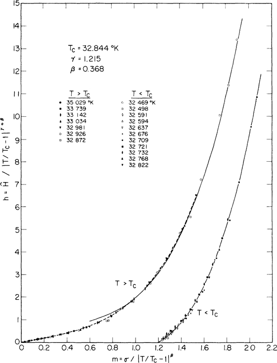
i.e., B/(|t|β+γ) is predicted to be a function f (with two branches f±, corresponding to t>0 and t<0) of the single variable |t|−βM(t,B). Equation (8.15) is a definite prediction of the scaling hypothesis, subject to validation. Figure 8.1 is a plot of the scaled magnetic field versus the scaled magnetization for the ferromagnet CrBr3[122]. The critical exponents β,γ were independently measured in zero field, the values of which were used to calculate the scaled field and magnetization. Measurements of M,B were made along isotherms for T<Tc and T>Tc, and the data beautifully fall on two curves. Figure 8.1 offers compelling evidence for the scaling hypothesis.
Figure 8.1Scaled magnetic field B/|t|β+γ versus scaled magnetization M/|t|β for the ferromagnet CrBr3. Reprinted figure with permission from J.T. Ho and J.D. Litster, Phys. Rev. Lett., 22, p. 603, (1969). Copyright (2020) by the American Physical Society.
The scaling hypothesis accounts for the relations we find among critical exponents and it has experimental support. It’s incumbent upon us therefore to find a microscopic understanding of scaling. We present the physical picture developed by L.P. Kadanoff[123] that provides a conceptual basis for scaling and which has become part of the standard language of critical phenomena.
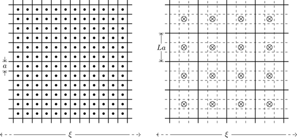
Consider a square lattice of lattice constant a, such as in the left part of Fig. 8.2, on which we have Ising spins (∙) coupled through nearest-neighbor interactions, with Hamiltonian
H=−J∑〈ij〉σiσj−b∑iσi,
(8.16)
Figure 8.2Two ways of looking at the same problem. Left: Square lattice of lattice constant a; circles (∙) represent Ising spins. In the critical region, ξ≫a. Right: Square lattice with scaled lattice constant La, such that L≪ξ/a; crosses ( ⊗) represent block spins. L=3 in this example.
where 〈ij〉 indicates a sum over nearest neighbors, on any lattice.5 In the critical region the correlation length ξ becomes macroscopic (critical opalescence, Section 6.7), implying the obvious inequality ξ≫a, yet this simple observation lies at the core of Kadanoff’s argument. So far, the lattice constant has been irrelevant in our treatment of phase transitions (often set to unity for convenience and forgotten thereafter). In many areas of physics, the length scale determining the relevant physics is fixed by fundamental constants.6 The correlation length ξ is an emergent length that develops macroscopic proportions as T→Tc, and is not fixed once and for all. A divergent correlation length in essence describes a new state of matter of highly correlated fluctuations.
Following Kadanoff, redefine the lattice constant, a→a′≡La, L≪ξ/a, an operation specifying a new lattice with the same symmetries as the original; the case for L=3 on the square lattice is shown in the right part of Fig. 8.2. On the original lattice there is one spin per unit cell. The unit cell of the scaled lattice contains Ld Ising spins, where we allow for an arbitrary dimension d, not just d=2 as in Fig. 8.2. That is, spins are still in their places; we’ve just redefined the unit of length (a scale transformation, or a dilatation). Label unit cells on the scaled lattice with capital Roman letters. Define a variable S˜I representing the degrees of freedom in the Ith cell,
S˜I≡∑i∈Iσi≈ξ≫La±Ld≡SILd,
(8.17)
where SI=±1 is a new Ising spin, the block spin (denoted ⊗ in Fig 8.2). Technically S˜I is a function of cell-spin configurations, S˜I=S˜I(σ1,⋯,σLd), having (Ld+1) possible values (show this). The two values assigned to S˜I in Eq. (8.17) represent the two cases of all cell spins correlated—all spins aligned—either up or down. Any other cell-spin configurations are unlikely to occur in the regime ξ≫La. The validity of the mapping in Eq. (8.17) that selects from the (Ld+1) possible values of S˜I, the two values ±Ld is therefore justified only when ξ≫La. Spins correlated over the size of a cell effectively act as a single unit—block spins.
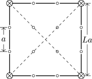
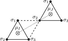
A key issue is the nature of interactions among block spins. Referring to Fig. 8.3, interactions between near-neighbor block spins (solid lines) are induced through the interactions of the spins on the original lattice (shown as open circles). New types of interactions, however, not in the original Hamiltonian are possible among block spins: next-near neighbor (dashed lines) or four-spin interactions. That is a complication we’ll have to address. For now, assume that block spins interact only with nearest neighbors and the magnetic field. Let’s write, therefore, a Hamiltonian for block spins:
HL≡−JL∑〈IJ〉SISJ−bL∑ISI,
(8.18)
Figure 8.3Block spins ( ⊗) interact with nearest neighbors (solid lines) through the nearest-neighbor couplings of the spins of the original lattice (open circles); next nearest neighbor interactions among block spins (dashed lines) can be mediated through the correlated spins of the cell.
where JL is the near-neighbor interaction strength between block spins associated with lattice constant La; likewise bL is the coupling of SI to the magnetic field. Clearly J1≡J and b1≡b. How we might calculate JL,bL will concern us in upcoming sections; for now we take them as given.
We’re considering, from a theoretical perspective, a change in the unit of length for systems in their critical regions, a→La, where ξ≫La>a. The correlation length is a function of K≡βJ, B≡βb, ξ=ξ(K,B). On the scaled lattice, ξ=ξ(KL,BL). Because it’s the same length, however, measured in two ways,7
ξ(KL,BL)=L−1ξ(K,B).
(8.19)
For N spins on the original lattice, there are N′≡N/Ld block spins on the scaled lattice. Because it’s the same system described in two ways, the free energy is invariant. Let g(t,B)≡G(t,B)/N denote the Gibbs energy per spin. Thus,
Ng(t,B)=N′g(tL,BL)⇒g(t,B)=L−dg(tL,BL),
(8.20)
where t=(Kc/K)−1. Equations (8.19) and (8.20) constrain the form of KL, BL; such relations hold only in the critical region, ξ≫La, and thus they apply for T near Tc and for small B.
Because ξ(KL,BL)<ξ(K,B) (Eq. (8.19)), the transformed system is further from the critical point (where ξ→∞). Let’s assume, in order to satisfy Eqs. (8.19), (8.20), that tL and BL are in the form
tL=LxtBL=LyB,
(8.21)
where x,y are new scaling exponents (independent of L). We require x,y>0 so that we move away from the critical point under a→La for L>1. Combining Eq. (8.21) with Eq. (8.20),
g(t,B)=L−dg(Lxt,LyB).
(8.22)
Under the assumptions of Kadanoff’s analysis, the free energy per spin is a generalized homogeneous function. Whereas Eq. (8.1) is posited to hold for an arbitrary mathematical parameter λ, the parameter L in Eq. (8.22) has physical meaning (and is not entirely arbitrary: L≪ξ/a). If we let L→L1/d, Eq. (8.22) has the form of Eq. (8.1):
g(t,B)=L−1g(Lx/dt,Ly/dB).
(8.23)
The exponents a,b in Eq. (8.1) correspond to Kadanoff’s exponents, a↔x/d and b↔y/d.
Kadanoff has shown therefore, for systems in their critical regions, how, if under a change in length scale a→La the couplings tL,BL transform as in Eq. (8.21), then the free energy exhibits Widom scaling. Of the two assumptions on which the theory rests, that block spins interact with nearest neighbors and tL, BL scale as in Eq. (8.21), the latter is most in need of justification, and we’ll come back to it (Sections 8.4, 8.6). The larger point, however, is that the block-spin picture implies a new paradigm, that changes in length scale (a spatial quantity) induce changes in couplings, thereby providing a physical mechanism for scaling.
We’ve noted previously (Section 6.5.3) the distinction between thermodynamic and structural quantities (correlation functions); the former can be derived from the free energy, the latter cannot. Kadanoff’s scaling picture, which links thermodynamic quantities with spatial considerations, can be used to develop a scaling theory of correlation functions, thereby relating the critical exponents ν,η to the others, α,β,γ,δ. Define the two-point correlation function for block spins,
C(rL,tL,BL)≡〈SISJ〉−〈SI〉〈SJ〉,
(8.24)
where rL is the distance between the cells associated with block spins SI, SJ (measured in units of La). Let r denote the same distance measured in units of a; thus, rL=L−1r (see Eq. 8.19). In order for block-spin correlations to be well defined, we require the inter-block separation be much greater than the size of cells, rL≫La⇒r≫L2a>a. A scaling theory of correlation functions is possible only for long-range correlations, r≫a.
In formulating the block spin idea, we noted in Eq. (8.17) the approximate correspondence SI≈L−d∑i∈Iσi. How accurate is that association, and does it hold the same for all dimensions d? Consider the interaction of the spin system with a magnetic field, supposing the inter-spin couplings have been turned off. Because we’re looking at the same system in two ways,
Equation (8.25) invites us to infer bL=bLd, which, comparing with Eq. (8.21), implies the scaling exponent y=d. If that were the case, it would imply the Widom scaling exponent b=y/d=1, and thus δ→∞ (Eq. (8.6)). To achieve consistency, we take, instead of Eq. (8.17),
SI=L−y∑i∈Iσi,
(8.26)
where we expect y≲d. Nowhere in our analysis did we make explicit use of Eq. (8.17).
Set B=0 in Eq. (8.29) and then let |t|=0. Correlation functions decay algebraically with distance at T=Tc (Section 7.6), and thus we identify, using Eq. (7.75),
2(d−y)=d−2+η⇒y=12(d+2−η).
(8.30)
Again set B=0; we know as |t|→0, long-range correlation functions are associated with the correlation length ξ. We require that r/ξ~r|t|ν=r|t|1/x, implying
x=1ν.
(8.31)
With these identifications of x,y, combined with the Widom scaling exponents x=ad, y=bd, and using the expressions for a,b in Eqs. (8.7), (8.11), there are numerous interrelations involving ν,η with the other critical exponents. For example, one can show
The Widom scaling hypothesis Eq. (8.1) accounts for relations among the exponents α,β,γ,δ. The block-spin picture (Section 8.2) motivates Eq. (8.1) and shows the exponents η,ν are related to α,β,γ,δ and d. The upshot is, that of the six critical exponents α,β,γ,δ,η,ν, only two are independent. That statement hinges on the validity of Eq. (8.21), Kadanoff’s scaling form for block-spin couplings. It’s time we got down to the business of calculating block-spin couplings, a process known as renormalization. We’ll see (Sections 8.4, 8.6) how understanding the physics behind Eq. (8.21) leads to a more general theory known as the renormalization group.8
8.3.1 Decimation method for one-dimensional systems
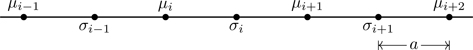
We start with the d=1 Ising model with near-neighbor couplings where we double the lattice constant, a system simple enough that we can carry out all steps exactly. Figure 8.4 shows a one-dimensional lattice with lattice constant a, with Ising spins σ on lattice sites, except that on every other site we’ve renamed the spins μ, which shall be the block spins. One way to define block spins (but not the only way) is simply to rename a subset of the original Ising spins, μ. One finds the interactions between μ-spins by summing over the degrees of freedom of the σ-spins in a partial evaluation of the partition function, a technique known as decimation. To show that, it’s convenient to work with a dimensionless Hamiltonian, H≡−βH. Thus, for the d=1 Ising model, H=K∑iσiσi+1+B∑iσi. Referring to Fig. 8.4, we can rewrite the Hamiltonian (exactly) assuming that even-numbered spins σ2i are named μi,
Figure 8.4One-dimensional lattice of lattice constant a; block spins are denoted μ.
where we’ve written the coupling of the μ-spins to the B-field in the form 12B(μi+μi+1) to “share” the μ-spins surrounding each odd-numbered σ-spin.9 For the partition function,
The strategy is to evaluate Eq. (8.34) in two steps: Sum first over the σ-degrees of freedom—a partial evaluation of the partition function—and then those associated with the μ-spins. The sum over σ2i+1 in Eq. (8.34) is straightforward:
Our goal is to exponentiate the terms we find after summing over σ2n+1, i.e., fit the right side of Eq. (8.35) to an exponential form. We want the following relation to hold:
Three parameters, K0,K′,B′, are required to match the three independent configurations of μn, μn+1: both up, ↑↑; both down, ↓↓; and anti-aligned, ↑↓ or ↓↑. We require
Thus, we have in Eq. (8.38) explicit expressions for K0,K′,B′; they are known quantities. Combining Eq. (8.36) with Eq. (8.34), we find
ZN(K,B)=∑{σ}eH=eNK0/2∑{μ}eH′=eNK0/2ZN/2(K′,B′),
(8.39)
where ∑{μ}≡∏i=1N/2∑μi=−11 and H′≡∑i=1N/2K′μiμi+1+B′μi. The quantities K′,B′ are known as renormalized couplings, with H′ the renormalized Hamiltonian.10 In stretching the lattice constant a→2a, we have at the same time “thinned,” or coarse grained, the number of spins N→N/2, which interact through effective couplings K′,B′. Equation (8.39) indicates that while the number of states available11 to the renormalized system is less than the original ( ZN/2<ZN), the equality ZN(K,B)=eNK0/2ZN(K′,B′) is maintained12 through the factor of eNK0/2, where we note that K0≠0, even if K=0 or B=0 (see (8.38)).
We’ve achieved the first part of the Kadanoff construction. Starting with a near-neighbor model with couplings K,B, we have, upon a→2a, another near-neighbor model with couplings K′,B′. By the scaling hypothesis, K′,B′ should occur further from the critical point at T=0, B=0 with K′<K and B′>B. To examine the recursion relationsK′=K′(K,B), B′=B′(K,B), it’s easier in this case (because Tc=0) to work with x≡e−4K and y≡e−2B, in terms of which the critical point occurs at x=0,y=1. With x′≡e−4K′, y′≡e−2B′, we find from (8.38) an equivalent form of the recursion relations
x′=x(1+y)2x(1+y2)+y(1+x2)y′=yy+x1+xy,
(8.40)
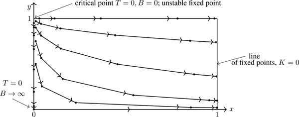
from which it’s readily shown that y′<y if y<1 and x′>x if x<1. Figure 8.5 shows the flows that occur under iteration of the recursion relations in (8.40). Starting from a given point in the x–y plane, the renormalized parameters do indeed occur further from the critical point.
Figure 8.5Flow of renormalized couplings for the d=1 Ising model, y≡e−2B, x≡e−4K. Arrows are placed 90% of the way to the next point.
We see from Fig. 8.5 that systems with coupling constants e−4K≪1 (for any B-field strength) are transformed under successive renormalizations into equivalent systems characterized by K=0. What may have been a difficult problem for K≫0 is, by this technique, transformed into an equivalent problem associated with K=0, which is trivially solved.13 What started as a way to provide a physical underpinning to scaling has turned into a method of solving problems in statistical mechanics. But, back to scaling. Let’s check if Eq. (8.21) is satisfied.
We start by examining the recursion relations (8.40) for the occurrence of fixed points, values x*,y* invariant under the block-spin transformation:
x*=x*(1+y*)2x*(1+y*2)+y*(1+x*2)y*=y*y*+x*1+x*y*.
(8.41)
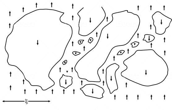
Analysis of (8.41) shows fixed points for x*=0,y*=1 —the critical point—and a line of “high temperature” fixed points x*=1 for all y. From Fig. 8.5, for K,B near the critical point, the renormalization flows are away from the fixed point, an unstable fixed point, and toward the high-temperature fixed points. We therefore have another way of characterizing critical points as unstable fixed points of the recursion relations for couplings.14 If for a fixed set of couplings (such as at a fixed point) there is no change in couplings under changes in length scale, the correlation length is the same for all length scales, implying fluctuations of all sizes, schematically illustrated in Fig. 8.6. The only way ξ can have the same value for any finite length scale is if ξ→∞. Unstable fixed points imply infinite correlation lengths. At the critical point (and only at the critical point) the system appears the same no matter what length scale you use to look at it. Such systems are said to be self-similar or scale invariant.15 The critical point is a special state of matter, indeed!
Figure 8.6At critical points ( ξ→∞) fluctuations of all sizes occur.
Scale invariance is not typical. In most areas of physics, an understanding of the phenomena requires knowledge of the “reigning physics” at a single scale (length, time, mass, etc.). For example, modeling sound waves in a gas of uranium atoms does not involve subatomic physics. One cannot start with a model of nuclear degrees of freedom, and arrive at the equations of hydrodynamics by continuously varying the length scale. Most theories apply at a definite scale, such as the mean free path between collisions. There are systems besides critical phenomena exhibiting scale invariance—fully developed turbulence in fluids[125][126], in elementary particle physics,16 and in fractal systems.17 Scale invariance is also observed in systems where the framework of equilibrium statistical mechanics does not apply, such as the jamming and yielding transitions in granular media [128, 129]
The recursion relations in (8.40) are nonlinear; let’s linearize them in the vicinity of a fixed point. Taylor expand18x′=x′(x,y), y′=y′(x,y) about x*,y*,
Defining δx≡x−x*, δy≡y−y*, and keeping terms to first order,
δx′δy′=∂x′/∂x*∂x′/∂y*∂y′/∂x*∂y′/∂y*δxδy=4002δxδy,
(8.43)
where we’ve evaluated at x*=0, y*=1 the partial derivatives of x′,y′ obtained from (8.40). The fixed point associated with the critical point is indeed unstable: Small deviations δx, δy from the critical point are, upon a→2a, mapped into larger deviations δx′, δy′. Are the relations in Eq. (8.43) in the scaling form posited by Eq. (8.21)? Because L=2 in this case, we can write (from Eq. (8.43)) δx′=L2δx and δy′=Lδy —nominally the scaling form we seek. The fact, however, that Tc=0 for d=1 complicates the analysis. For small B (near the critical point), δy≡y−1≈−2B; thus δy′=Lδy implies B′=LB≡LysB, where ys denotes the Kadanoff scaling exponent (to distinguish it from the variable y in use here). Thus, we find ys=1 for the d=1 Ising model. Comparing with Eq. (8.30), we see that ys=1 is precisely what we expect because η=1 exists for d=1 (see Exercise 8.1). For the coupling K, e−4K′=4e−4K (Eq. (8.43)) implies K′=K−12ln2 (for large K). Thus, ∂K′/∂K*=1=L0, implying the scaling exponent xs=0, which in turn implies ν→∞ from Eq. (8.31). The critical exponent ν can’t be defined for d=1 because ξ doesn’t diverge as a power law, but rather exponentially; see Eq. (P6.1). Kadanoff scaling holds in one dimension, but we need to find the “right” scaling variables, here δx,δy.
The scaling form tL=Lxt (Eq. (8.21)) is written in terms of t≡(T−Tc)/Tc, where |t|→0 as T→Tc. We can, equivalently, develop a scaling variable involving K=J/(kT), with
KL=Kc−(Kc−K)Lx.
(8.44)
Equation (8.44) indicates that (Kc−K) is the quantity that gets small near the critical point;19 see Exercise 8.20. We’ve been writing KL,BL in this section as K′,B′. Using Eq. (8.44) and BL=LyB from Eq. (8.21), we can infer the critical exponents η,ν by connecting these scaling forms with Eqs. (8.30) and (8.31):
The exponents η,ν can be calculated from the recursion relations at unstable fixed points. Once they’re known, the other exponents follow (only two are independent). The renormalization method predicts Kc from the fixed point of the transformation, and, by connecting critical exponents with fixed-point behavior, scaling emerges from the linearized recursion relations at the fixed point. The Kadanoff construction, devised to support the scaling hypothesis, turns out to represent a more comprehensive theory (see Section 8.4).
Let’s see what else we can do with recursion relations besides finding critical exponents. Define a dimensionless free energy per spin, F≡limN→∞−βF/N=limN→∞1NlnZN. Combining F with Eq. (8.39),
F=12K0+12F′,
(8.46)
where F′≡F(K′,B′). Make sure you understand the factor of 12 multiplying F′ in Eq. (8.46). Let’s iterate Eq. (8.46) twice:
where K0(m)≡K0(K(m),B(m)) denotes the mth iterate of K0, with K0(0)≡K0(K,B). Under successive iterations, K,B are mapped into fixed points at K=0 and some value B=B*. From (8.38), K0(K=0,B)=ln2coshB. For the Ising model F=lnλ+, where λ+ is the largest eigenvalue of the transfer matrix. At the high-temperature fixed point, λ+=2coshB* (Eq. (6.82)). Thus, F is mapped into F=ln(2coshB*), and hence the sum in Eq. (8.47) converges as N→∞,
F(K,B)=∑n=0∞12n+1K0K(n),B(n).
(8.48)
Renormalization provides a way to calculate the free energy not involving a direct evaluation of the partition function—it’s a new paradigm in statistical mechanics. The function K0, the “constant” in the renormalized Hamiltonian, is essential for this purpose, as are the recursion relations K′=K′(K,B), B′=B′(K,B). Non-analyticities arise in the limit of an infinite number of iterations of recursion relations, in which all degrees of freedom in the thermodynamic limit have been summed over, as if we had exactly evaluated the partition function.
Recursion relations can be developed for quantities derivable from the free energy by taking derivatives. For the magnetization per spin m≡∂F/∂BK (see Eq. (6.84)), we have by differentiating Eq. (8.46):
m=12∂K0∂B+12∂B′∂Bm′.
(8.49)
For the zero-field susceptibility per spin χ=∂m/∂BB=0,
χ=12∂2K0∂B2B=0+12∂B′∂BB=02χ′.
(8.50)
It’s straightforward to write computer programs to iterate recursion relations such as these.
8.3.2 Decimation of the square-lattice Ising model
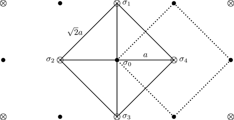
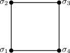
Let’s try decimation on the square lattice for an Ising model having nearest-neighbor interactions in the absence of a magnetic field. From Fig. 8.7, a square lattice of lattice constant a can be decomposed into interpenetrating sublattices,20 square lattices of lattice constant 2a that have been rotated 45∘ relative to the original.21,22 Let spins on one sublattice be the block spins. Interactions between them can be inferred by summing out the degrees of freedom associated with the other sublattice. Referring to Fig. 8.7, we sum over σ0:
Figure 8.7Square lattice of lattice constant a decomposed into interpenetrating square sublattices of circles (∙) and crosses ( ⊗), each having lattice constant 2a.
Just as with Eq. (8.35), our job is to fit the right side of Eq. (8.51) to an exponential form:
where, in addition to K0, we’ve allowed for nearest-neighbor couplings K1 (the factor of 12 is because these interactions are “shared” with neighboring cells), next-nearest neighbor couplings K2, and a four-spin interaction, K4. Four parameters are required to match the four independent energy configurations of σ1,σ2,σ3,σ4: ↑↑↑↑, ↑↑↑↓, ↑↑↓↓, ↑↓↑↓. Thus, from Eq. (8.52),
Thus, starting with a near-neighbor model on the square lattice, we’ve found, using decimation, a model on the scaled lattice having near-neighbor interactions in addition to next-nearest-neighbor and four-spin couplings. To be consistent, we should start over with a model having first, second neighbor and four-spin interactions.23 If one does that, however, progressively more types of interactions are generated under successive transformations. K.G. Wilson found[130] that more than 200 types of couplings are required to have a consistent set of recursion relations for the square-lattice Ising model.24 For that reason, decimation isn’t viable in two or more dimensions.25 We’d still like a way, however, to illustrate renormalization in two dimensions as there are new features to be learned. We develop in Section 8.3.4 an approximate set of recursion relations for the square lattice. Before doing that, we touch on a traditional approach to critical phenomena, the method of high-temperature series expansions.
8.3.3 High-temperature series expansions—once over lightly
Suppose the temperature is such that kT≫H[σ1,⋯,σN] for all spin configurations. In that case one could try expanding the Boltzmann factor in a Taylor series,
where for any spin function, 〈f(σ)〉0≡(1/2N)∑{σ}f(σ) denotes an average with respect to the uniform probability distribution, 2−N. In terms of the average symbol 〈〉0,
ZN=2N〈e−βH〉0.
(8.56)
Example. As an example, consider a system of three Ising spins arranged on the vertices of an equilateral triangle, with Hamiltonian H=−J(σ1σ2+σ2σ3+σ3σ1). Then,
〈H〉0=−J18∑σ1=−11∑σ2=−11∑σ3=−11σ1σ2+σ2σ3+σ3σ1=0.
As one can show, H2=J23+2σ1σ2+2σ2σ3+2σ3σ1, and thus
Through second order in a high-temperature series, Z3=8(1+32K2+⋯), where K≡βJ.
We obtain the partition function in statistical mechanics to calculate averages, a step facilitated by working with the free energy, −βF=lnZN. From Eq. (8.56),
where the quantities Cn are cumulants (see Sections 3.7 and 6.3). Equation (8.57) is identical to Eq. (6.38) when we identify −βFideal with Nln2. Explicit expressions for cumulants in terms of moments are listed in Eq. (3.62), e.g., C1=〈H〉0 and C2=〈H2〉0−〈H〉02. The values of the cumulants Cn depend on the range of the interactions and the geometry of the lattice.26 There is an extensive literature on high-temperature series expansions. To give just one example, 54 terms are known for the high-temperature series of the susceptibility of the square-lattice Ising model [132]. With high-temperature series, we’re expanding about the state of uncoupled spins, K=0. Can one find information this way about thermodynamic functions exhibiting singularities at K=Kc ? Indeed, that’s the art of this approach27—extracting information about critical phenomena at K=Kc from a finite number of terms in a Taylor series about K=0.
Series expansions can be developed for correlation functions, and to do that we introduce another approach to the partition function. For a nearest-neighbor Ising model ( H=−J∑〈ij〉σiσj),
ZN=∑{σ}e−βH=∑{σ}eK∑〈ij〉σiσj=∑{σ}∏〈ij〉eKσiσj.
(8.58)
We use the following identity for Ising spins, not necessarily near-neighbor pairs,
eKσkσl= coshK+σkσlsinhK= coshK1+uσkσl,
(8.59)
where u≡tanhK. Combining Eq. (8.59) with Eq. (8.58),
ZN= coshPK∑{σ}∏〈ij〉1+uσiσj,
(8.60)
where P is the number of distinct near-neighbor pairs on the lattice.28 For systems satisfying periodic boundary conditions, P=Nz/2 where z is the coordination number of the lattice. There are P factors of (1+uσiσj) in the product in Eq. (8.60).
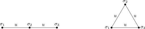
Let’s illustrate Eq. (8.60) with some simple cases. Figure 8.8 shows two, three-spin Ising systems, one with free boundary conditions and the other with periodic boundary conditions. For free boundary conditions, there are two near-neighbor pairs ( P=2), and thus expanding (1+uσ1σ2)(1+uσ2σ3) in Eq. (8.60),
Figure 8.8Three-spin Ising systems with free boundary conditions (left) and periodic boundary conditions (right). Each near-neighbor bond is given weight u=tanhK.
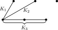
It helps to draw a line connecting the spins in each near-neighbor pair, as in Fig. 8.8. Referring to these lines as “bonds,” we associate a factor of u=tanhK with each bond. Before summing over spins in Eq. (8.61), we see a connection between spins σ1, σ3 of strength u2; terms like this occur when, in expanding the product in Eq. (8.60), we have “overlap” products such as (uσ1σ2)(uσ2σ3)=u2σ1σ3. In the left part of Fig. 8.8 there are two bonds between σ1 and σ3—one between σ1,σ2 and the other between σ2,σ3. We multiply the bond strengths for each link in any lattice-path connecting given spins consisting entirely of nearest-neighbor pairs.29
For periodic boundary conditions in Fig. 8.8, P=3 and thus from Eq. (8.60),
Before summing over spins in Eq. (8.62) and referring to the right part of Fig. 8.8, we see a direct near-neighbor connection between spins σ1, σ2 of strength u, and another connection between σ1, σ2 of strength u2 mediated by the path through σ3. We also see a new feature in Eq. (8.62): a coupling of strength u3 associated with a closed path of near-neighbor links from the overlap product (uσ1σ2)(uσ2σ3)(uσ3σ1)=u3. Note that Eq. (8.61) agrees with Eq. (6.71) for N=3, while Eq. (8.62) agrees with Eq. (6.81) for N=3.
We can now see how expansions for correlation functions are developed. Consider, for any spins σl, σm, that for a nearest-neighbor Ising model,
where we’ve used Eq. (8.62) for Z3pbc. In the second equality in Eq. (8.64), we’ve listed in square brackets only the terms proportional to the spin product σ1σ3. We have in Eq. (8.64) the exact result for 〈σ1σ3〉 (simple enough in this case to obtain through direct calculation), and, in the final equality, the first two terms in a high-temperature series expansion, valid for u≪1. The general process is clear: Somewhere in the expansion of the product in Eq. (8.63), there are terms involving the product σlσm. Only those terms survive the summation over spins in Eq. (8.63). One must find all lattice-paths connecting σl, σm consisting entirely of near-neighbor links.
8.3.4 Approximate recursion relations for the square-lattice Ising model
Let’s return to the square-lattice Ising model. In Section 8.3.2, we found that a near-neighbor model leads, under decimation, to a model with next-nearest neighbor and four-spin interactions. In this section we analyze a simplified, approximate set of recursion relations valid at high temperature for a model with nearest and next-nearest-neighbor interactions.30
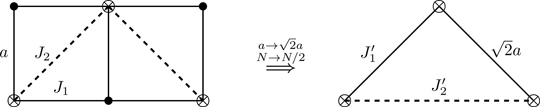
The left part of Fig. 8.9 shows part of a square lattice (lattice constant a) having near-neighbor interactions J1 (solid lines) and next-near-neighbor interactions J2 (dashed lines). Under the block-spin transformation ( a→2a and the number of spins N→N/2), we seek near and next-near-neighbor interactions J1′, J2′ (solid and dashed lines, right part of Fig. 8.9). There is “already” a direct interaction J2 between the spins we’re calling block spins ( ⊗-spins, left part of Fig. 8.9). On the scaled lattice, that interaction (J2 on the original lattice) is a partial contribution to the coupling J1′ between near-neighbor ⊗-spins. There is another contribution to J1′ from the near-neighbor couplings on the original lattice, 2J12 at high temperature—there are two near-neighbor links separating near-neighbor ⊗-spins, and there are two such paths connecting them (see Section 8.3.3 for this reasoning). For the second-neighbor interaction J2′, there is a contribution J12 (at high temperature) from the two nearest-neighbor links between ⊗-spins (left part of Fig. 8.9), in addition to an indirect contribution J22. Working with dimensionless parameters, we simply write down the recursion relations
K1′=2K12+K2K2′=K12,
(8.65)
Figure 8.9Left: Square lattice with nearest and next-nearest-neighbor interactions J1, J2 (solid and dashed lines). Right: Scaled lattice with nearest and next-nearest-neighbor interactions J1′, J2′.
where K22 has been dropped (from K2′) because it’s higher order in K. We have in (8.65) a consistent set of recursion relations at lowest order in K for the square lattice. They can be considered model recursion relations having enough complexity to illustrate more general recursion relations.
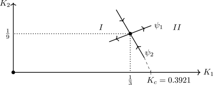
The first thing to do is find the fixed points. As is readily shown, the nontrivial fixed point is K1*=13, K2*=19. Next, we study the flows in the vicinity of that fixed point. Referring to Eq. (8.43), we have using Eq. (8.65) the linearized transformation
With Eq. (8.66) we encounter a new feature—the matrix representing the linearized transformation is not diagonal, as in Eq. (8.43). To find the appropriate scaling variables, we must work in a basis in which the transformation matrix is diagonal.
The eigenvalues of the matrix in Eq. (8.66) (easily found) are:
λ1=132+10≈1.721λ2=132−10≈−0.387,
(8.67)
where it’s customary to list the eigenvalues in descending order by magnitude, |λ1|>|λ2|. The associated eigenvectors (in the K1,K2 basis) are:
ψ1=10.387ψ2=1−1.721.
(8.68)
Figure 8.10 shows the fixed points of (8.65) in the K1,K2 plane, and the directions of the eigenvectors ψ1,ψ2 at the nontrivial fixed point. Because λ1>1, the fixed point is unstable for deviations δK1,δK2 lying in the direction associated with ψ1: small deviations in the direction of ψ1 (positive or negative) are mapped into larger deviations. For deviations δK1,δK2 lying in the direction of ψ2, however, the fixed point is stable—deviations are mapped closer to the fixed point ( |λ2|<1). Region I in Fig. 8.10 represents couplings that are mapped under iteration to the high-temperature fixed point. In Region II, couplings are mapped to “infinity.” Shown as the dashed line in Fig. 8.10 is the extension to K2=0 of the line separating regions I,II, which occurs at K1≡Kc≈0.3921. Initial couplings K2=0, K1<Kc are mapped into the high-temperature fixed point; initial couplings K2=0, K1>Kc flow to infinity (see Exercise 8.28). If one started with couplings K1=Kc, K2=0 (i.e., a near-neighbor model), one would have in a few iterations of (8.65) an equivalent model with the fixed-point couplings K1*,K2* (and it’s the fixed point that controls critical phenomena). Thus, this method predicts Kc≈0.3921 for the near-neighbor square-lattice Ising model, within 11% of the exact value Kc=12sinh−1(1)≈0.4407, Eq. (7.125), and distinct from the predictions of mean field theory on the square lattice, Kc=0.25 (see Section 7.8). That’s not bad considering the approximations in setting up Eq. (8.65), and is therefore encouraging: It compels us to find better ways of doing block-spin transformations (see Section 8.5). Prior to the renormalization method, there was no recourse to mean field theory other than exact evaluations of partition functions, nothing in the middle; now we have a method, a path, by which we can seek better approximations in terms of how we do block-spin transformations.31
Figure 8.10Fixed points (•) of the recursion relations (8.65). Shown are the directions of the eigenvectors ψ1 (positive eigenvalue) and ψ2 (negative eigenvalue) of the linearized transformation (see (8.68)). Initial points in region I flow under iteration to the high-temperature fixed point; those in region II flow to larger values of K1,K2 (where the model isn’t valid). Kc≈0.3921 is the numerically obtained extension to K2=0 of the line separating regions I, II (dashed line).
We find critical exponents from linearized recursion relations at fixed points, as in Eq. (8.45). Equation (8.45), however, utilized the diagonal transformation matrix Eq. (8.43) and must be modified for non-diagonal matrices as in Eq. (8.66). If we work in a basis of eigenvectors, the transformation matrix is diagonal with eigenvalues along the diagonal. Thus, instead of Eq. (8.45),
ν=1x=lnLlnλ1.
(8.69)
With L=2 and λ1=1.721 (Eq. (8.67)), we find ν≈0.638. Again, not the exact value ν=1, but also not the mean field theory exponent, ν=12 (see Table 7.3). Given the approximations, ν=0.638 is an encouraging first result, and will improve as we get better at block-spin transformations.
We now look at renormalization from a more general perspective. We start by enlarging the class of Hamiltonians to include all the types of spin interactions Si(σ) generated by renormalization transformations,32
−βH=H=∑iKiSi(σ).
(8.70)
We could have the sum of spins S1≡∑k=1Nσk, near-neighbor two-spin interactions S2,nn≡∑〈ij〉σiσj, next-nearest neighbor two-spin interactions S2,nnn≡∑ij∈nnnσiσj, three, and four-spin interactions, etc. See Exercise 8.29. All generated interactions must be included in the model to have a consistent theory (see Section 8.3.2). We can collect these interactions in a set {Si} labeled by an index i. As we’ve learned (Section 8.3), we should include a constant in the Hamiltonian; call it S0≡1. The couplings Ki in Eq. (8.70) are dimensionless parameters associated with spin interactions Si. In what follows, we “package” the couplings {Ki} into a vector, K≡(K0,K1,K2,⋯). A system characterized by couplings (K0,K1,⋯) is represented by a vector K in a space of all possible couplings, coupling space (or parameter space).
Renormalization transformations have two parts: 1) stretch the lattice constant a→La and thin the number of spins N→N/Ld; and 2) find the effective couplings K′ among the remaining degrees of freedom (such that Eqs. (8.19) and (8.20) are satisfied). Starting with a model characterized by couplings K, find the renormalized couplings K′, an operation that we symbolize
K′=RLK.(L>1)
(8.71)
That is, RL is an operator that maps the coupling vector K to that of the transformed system K′ associated with scale change L. Representing renormalizations with an operator is standard,33 but it’s abstract. An equivalent but more concrete way of writing Eq. (8.71) is
Ki′=fi(L)(K),
(8.72)
where i runs over the range of the index in Eq. (8.70). For each renormalized coupling Ki′ associated with scale change L, there is a function fi(L) of all couplings K (see Eqs. (8.38), (8.40), or (8.65)). RL is thus a collection of functions that act on the components of K, RL↔{fi(L)}. We’ll use both ways of writing the transformation.
A renormalization followed by a renormalization is itself a renormalization; let’s show that. Starting from a model characterized by couplings K, do the transformation with L=L1, followed by another with L=L2. Then, with K′=RL1(K) and K′′=RL2(K′),
K′′=RL2(K′)=RL2·RL1(K)≡RL2×L1(\bmK).
(8.73)
The compound effect of two successive transformations (of scale changes L1,L2) is equivalent to a single transformation with the product L1L2 as the scale change factor. Equation (8.73) implies the operator statement,
RL2·RL1=RL2L1.
(8.74)
Equation (8.74) indicates that the order in which we perform renormalizations is immaterial, i.e., renormalizations commute: RL1L2=RL2L1⇒RL1·RL2=RL2·RL1. This must be the case—we’re rescaling the same lattice structure (having the same symmetries), the order in which we do that is immaterial. Equation (8.74) is the group property, a word borrowed from mathematics. A group is a set of mathematical objects (elements) equipped with a binary operation such that the composition of any two elements produces another member of the set, such as we see in Eq. (8.74) for the set of all renormalization transformations {RL≥1}. For that reason, the theory of renormalization is referred to as renormalization group theory, even though renormalizations do not constitute a group! To be a group, the set must satisfy additional criteria,34 the most important of which for our purposes is that for each element of the set, there exists an inverse element in the set.35 Renormalizations possess the group composition property, Eq. (8.74), but they do not possess inverses. The operator RL is defined for L>1 (Eq. (8.71)) and not for 0<L<1; a definite “one-sided” progression in renormalized systems is implied by the requirement L>1. Once we’ve coarse-grained the number of spins N→N/Ld, there’s no going back—we can’t undo the transformation. Sets possessing the attributes of a group except for inverses are known as semigroups. The term renormalization group is a misnomer, but that doesn’t stop people (like us) from using it.
Critical phenomena are associated with the behavior of recursion relations in the vicinity of fixed points (Section 8.3). Fixed points are solutions of the set of equations (from Eq. (8.72))36
Ki*=fi(L)(K*).
(8.75)
Solutions of Eq. (8.75) may be isolated points in K-space, or solution families parameterized by continuous variables, or it may be that Eq. (8.75) has no solution. In what follows, we assume that a solution K* is known to exist at an isolated point.
In the vicinity of the fixed point, we have, generalizing the relations in (8.42),
δKi′=∑j∂fi(L)∂Kj*δKj≡∑jRij(L)δKj,
(8.76)
where Rij(L) are the elements of the linearized transformation matrix R(L). The matrix R(L) is in general not symmetric and may not be diagonalizable; even if it is diagonalizable, it may not have real eigenvalues. We assume the simplest case that R(L) is diagonalizable with real eigenvalues.
The eigenvalue problem associated with R(L) can be written
∑jRij(L)ψj(k)=λk(L)ψi(k),
(8.77)
where k labels the eigenvalue λk(L) of RL associated with eigenvector ψ(k) (having ψj(k) as its jth component). We don’t label the eigenvectors in Eq. (8.77) with L because renormalizations commute. Equation (8.74), which holds for any renormalizations, holds for the linearized version involving matrices,
R(L1)R(L2)=R(L1L2),
(8.78)
and thus, because commuting operators have a common set of eigenvectors, but not eigenvalues,37 we can’t label eigenvectors with L. Equation (8.78) implies for eigenvalues (see Exercise 8.30)
λk(L1)λk(L2)=λk(L1L2).
(8.79)
Equation (8.79) is a functional equation for eigenvalues; it has the solution
λk(L)=Lyk,
(8.80)
where the exponent yk is independent of L. Equation (8.80) is a strong prediction of the theory: The eigenvalues occur in the scaling form posited in Eq. (8.21). By setting L2=1 in Eq. (8.79), we find λk(1)=1 (the L=1 transformation is the identity transformation), and thus we have the explicit scaling relation λk(L)=Lykλk(1). Scaling in the form assumed by Kadanoff occurs quite generally, relying only on the existence of fixed points and the group property, Eq. (8.74).
Scaling fields qk are vectors in K-space (coupling space) obtained from linear combinations of the deviations δKi, weighted by eigenvector components,38
qk≡∑lψl(k)δKl.
(8.81)
In terms of these variables (scaling fields), the linearized recursion relations decouple (instead of their form in Eq. (8.76)),
qk′=λk(L)qk=Lykqk,
(8.82)
where we’ve used Eq. (8.80) (see Exercise 8.31). Scaling fields are classified as follows:
Scaling fields qk with |λk|>1 ( yk>0) are termed relevant. Under iteration, relevant scaling fields grow in magnitude, qk′>qk, with the new couplings K′ further removed from the critical point at K* than the original K;
Scaling fields qk with |λk|<1 ( yk<0) are termed irrelevant. Under iteration, qk′<qk; the new couplings K′ are closer to K* than the original K;
Scaling fields qk with |λk|=1 ( yk=0) are termed marginal. In the linear approximation, such variables neither grow nor decrease in magnitude under iteration. Further analysis is required to ascertain the fate of such variables under many iterations.
After many iterations, only the components of δK along the direction of relevant scaling fields will matter; components of δK along irrelevant or marginal scaling fields will either shrink or stay fixed at a finite value. The manifold spanned by irrelevant scaling fields is called the critical manifold, the existence of which accounts for universality, that different physical systems can exhibit the same critical phenomena (see Section 7.3.2). Irrelevant variables are simply that—irrelevant for the purposes of describing critical phenomena. Couplings K not lying in the critical manifold flow under successive iterations away from it. Measurable critical phenomena are associated with relevant variables. It’s found that most interactions are irrelevant; critical phenomena are determined by a few relevant variables which can be grouped into universality classes determined by the dimensionality and the symmetries of the system.39
Renormalization group theory systematizes the framework of block-spin transformations and shows that the Kadanoff scaling form, Eq. (8.21), is exhibited by the eigenvalues of the linearized transformation matrix, Eq. (8.80). It should be kept in mind that the functions fi(K) on which the method is based (see Eq. (8.72)) can no more be found in general than we can evaluate partition functions. A strength of the renormalization approach is that the functions fi(K) are expected to be analytic, and hence amenable to approximation. Singularities associated with phase transitions occur only in the thermodynamic limit (Section 7.10), implying the need (in traditional statistical mechanics) to find the exact free energy as a function of N. In the renormalization method, singularities are built up iteratively. Two complementary approaches to the functions fi(K) have been developed: lattice-based methods (real space or position space renormalization), and field-theoretic methods (momentum space or k-space renormalization) that work with continuous spin fields. We treat the former in the next section and touch on the latter in Section 8.6.
Consider a set {σ} of N interacting Ising spins on a lattice of lattice constant a, and suppose we wish to find a new set {μ} of N′ Ising spins and their interactions on a scaled lattice with lattice constant La, where N′=N/Ld. For that purpose, we define the real space mapping functionT[μ|σ], such that
eH′(μ)=∑{σ}T[μ|σ]eH(σ).
(8.83)
A requirement on the function T[μ|σ] is that
∑{μ}T[μ|σ]≡∏i=1N′∑μi=−11T[μ|σ]=1.
(8.84)
Equation (8.84) implies, from Eq. (8.83), that
ZN′(K′)=ZN(K).
(8.85)
Equation (8.85) appears to differ from Eq. (8.39), but there is no discrepancy: In (8.39) we separated the constant term N′K0 from the renormalized Hamiltonian H′; in (8.85) the generated constant is part of H′. By combining Eq. (8.85) with Eq. (8.83), we have for the block-spin probability distribution P(μ),
P(μ)=〈T[μ|σ]〉.
(8.86)
The quantity T[μ|σ] therefore plays the role of a conditional probability (Section 3.2) that the μ-spins have their values, given that the configuration of σ-spins is known.
In principle there is a renormalization transformation for every function T[μ|σ] satisfying Eq. (8.84); in practice there are a limited number of forms for T[μ|σ]. Defining transformations as in Eq. (8.83) (with a mapping function) formalizes and generalizes the decimation method, to which it reduces if T[μ|σ] is a product of delta functions. The transformation studied in Section 8.3.1 is effected by Eq. (8.83) if T[μ|σ]=∏i=1N/2δμi,σ2i. We now illustrate the application of Eq. (8.83) to the triangular-lattice Ising model.
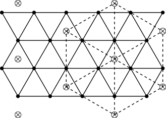
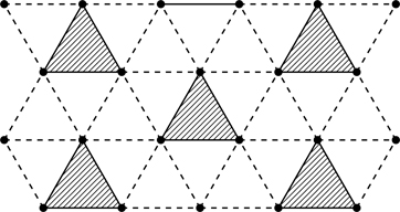
Figure 8.11 shows part of a triangular lattice with Ising spins (•) on its vertices (solid lines). A new triangular lattice for block spins (⊗) can be formed by dilating the original with L=3 and rotating it 30∘ (dashed lines). Figure 8.12 shows groups (in crosshatching) of three σ-spins that form the coarse-graining cells in which their degrees of freedom are mapped into those of the block spin. Every σ-spin is uniquely associated with one of these cells. As explained below, we distinguish intracell couplings (solid lines) and intercell couplings between σ-spins in near-neighbor cells (dashed lines). By writing T[μ|σ] as a product of cell mapping functions Ti[μ|σ],
T[μ|σ]≡∏i=1N′Ti[μ|σ],
(8.87)
Figure 8.11Part of 1) a triangular lattice (solid lines) with Ising spins (•), and 2) another triangular lattice (dashed lines) for block spins (⊗) scaled by L=3 and rotated 30∘.
Figure 8.12Three-spin coarse-graining cells on the triangular lattice (crosshatching). Intracell couplings indicated with solid lines; intercell couplings with dashed lines.
Eq. (8.84) is satisfied with
Ti[μ|σ]≡12(1+μiψ({σ}i)),
(8.88)
where ψ is a function of the cell spins {σ}. We will assume Eqs. (8.87) and (8.88) in what follows.
There is flexibility in the choice of ψ. Niemeijer and van Leeuwen[ 139 ] chose for the triangular lattice the so-called majority rule function,
ψσ1,σ2,σ3≡12(σ1+σ2+σ3−σ1σ2σ3),
(8.89)
where σ1,σ2,σ3 are the three σ-spins in each cell; see Fig. 8.13. There are four independent configurations of σ1,σ2,σ3: ↑↑↑,↑↑↓,↑↓↓,↓↓↓, for which ψ in Eq. (8.89) has the values ψ(↑↑↑)=1, ψ(↑↑↓)=1, ψ(↑↓↓)=−1, and ψ(↓↓↓)=−1. We note that the Kronecker delta function has the representation in Ising variables, δσ,σ′=121+σσ′. Comparing with Ti[μ|σ] in Eq. (8.88), we see that the majority-rule function with ψi=±1 generalizes the decimation method with T[μ|σ]=∏i=1N′δμi,ψi. Another approach, that of Mazenko, Nolan, and Valls[140], is to map onto the block spin the slowest dynamical mode of cell spins.40
Figure 8.13Interaction between nearest-neighbor block spins μI, μJ (dotted line).
Real-space renormalization based on mapping functions T[μ|σ] is more in keeping with the intent of the block-spin transformation (a mapping of cell degrees of freedom onto block spins) than is decimation (a renaming of a subset of the original spins as block spins). If decimation generates an apparently unending set of new interactions on two-dimensional lattices (Section 8.3.2), does real-space renormalization (a generalization of decimation) sidestep that problem? As we show, the use of perturbation theory allows us, if not to sidestep the problem, to forestall it and make it more systematic. We treat intracell couplings exactly (solid lines in Fig. 8.12), and intercell couplings (dashed lines) perturbatively. To do that, we divide the Hamiltonian H(σ) into a term H0(σ) containing all intracell interactions and a term V(σ) containing all intercell interactions:
That is, 〈〉0 denotes an average with respect to the probability distribution eH0(σ)T[μ|σ]/Z0, which is normalized with respect to σ-variables. From Eq. (8.93), we have the renormalized Hamiltonian
H′=lnZ0+ln〈eV〉0.
(8.95)
Hopefully you recognize the next step: ln〈eV〉 is the cumulant generating function (see Eqs. (3.60), (6.39), or (8.57)). Thus,
H′=lnZ0+∑n=1∞1n!Cn(〈V〉0),
(8.96)
where the Cn are cumulants ( C1=〈V〉0 and C2=〈V2〉0−〈V〉02; Eq. (3.62)).
We must therefore evaluate Z0 and the cumulants Cn. We first note that for each three-spin cell,
There is no μ-dependence to Z0 (in this case) because of up-down symmetry in the absence of a magnetic field. Using Eq. (8.90), we have the first cumulant
C1=〈V〉0=K∑〈IJ〉∑i∈I∑j∈J〈σi(I)σj(J)〉0.
(8.99)
Referring to Fig. 8.13, let’s work out the generic term:
Because the probability distribution eH0(σ)T[μ|σ]/Z0 factorizes over cells, the average we seek is a product of cell averages, 〈σ1(I)σ2(J)〉0=〈σ1(I)〉0〈σ2(J)〉0. We must evaluate
where we’ve used Eqs. (8.88) and (8.97) and the result of Exercise 8.36.
By combining Eq. (8.101) with Eq. (8.100), and then with Eq. (8.99), we have from Eqs. (8.96) and (8.98) the renormalized Hamiltonian to first order in the cumulant expansion:
H′=N′ln(e3K+3e−K)+K′∑〈IJ〉μIμJ,
(8.102)
where
K′=2Ke3K+e−Ke3K+3e−K2.
(8.103)
The factor of two in Eq. (8.103) comes from the two dashed lines connecting near-neighbor cells in Fig. 8.13. Now that we have the recursion relation K′=K′(K), what do we do with it? Hopefully you’re saying: Find the fixed point and then linearize. First, we observe from Eq. (8.103) that K′≈12K for K→0, i.e., K′ gets smaller for small K (high temperature), and K′≈2K for large K, i.e., K′ gets larger at low temperature. There must be a value K* such that K*′=K*, the nontrivial solution of
K*=2K*e3K*+e−K*e3K*+3e−K*2.
(8.104)
The fixed point K*≈0.336 should be compared with the exact critical coupling of the triangular-lattice Ising model, Kcexact=14ln3≈0.275 [142],41 and the prediction of mean field theory, Kcmeanfield=16≈0.167 (Section 7.9). It’s straightforward to evaluate from Eq. (8.103)
∂K′∂K*≈1.624.
(8.105)
We then have, using Eq. (8.45), the critical exponent ν:
ν=lnLln∂K′/∂K*=ln3ln1.624≈1.133,
(8.106)
a result not too far from the exact value ν=1 and distinct from the prediction of mean field theory, ν=12 (see Table 7.3). Note that to have ν=1, we “want” ∂K′/∂K*=3≈1.732.
The next step is to evaluate the cumulant C2 to see whether the expansion in Eq. (8.96) leads to better results. These are laborious calculations; we omit the details and defer to [139]. In calculating C2, next-nearest and third-neighbor interactions are generated, call them K2,K3, in addition to near-neighbor couplings, which we now call K1. Figure 8.14 shows these interactions on the triangular lattice. One must start with a model having couplings K1,K2,K3 on the original lattice to calculate K1′,K2′,K3′ on the scaled lattice. We omit expressions for the recursion relations Ki′=fi(K), i=1,2,3 (included in f1 are the results obtained at first order in the cumulant expansion, Eq. (8.103)). As per Niemeijer and van Leeuwen[ 139 ], the nontrivial fixed point is at K*≡(K1*=0.2789,K2*=−0.0143,K3*=−0.0152), with the transformation matrix
Figure 8.14Near, next-nearest, and third-neighbor couplings K1,K2,K3 on the triangular lattice.
having eigenvalues λ1=1.7835, λ2=0.2286, λ3=−0.1156. There is one relevant and two irrelevant scaling fields. We see that λ1 is closer to λ1exact=3 than for C1, ≈1.624. As in Section 8.3.4, the line separating flows to the high and low-temperature fixed points can be extended to K2=K3=0 at Kc=0.2514, closer to Kcexact=0.275 than for C1, ≈0.336. From Eq. (8.69), ν=ln3/lnλ1≈0.949, closer to the exact result ν=1 than in Eq. (8.106).
Working to second order in the cumulant expansion therefore provides improved results for the triangular lattice. A third-order cumulant calculation on the triangular lattice found improvements over second-order results[143], and thus “so far, so good,” it might appear that the cumulant expansion is a general method of real-space renormalization. The convergence of the expansion, however, is not understood—the series in Eq. (8.96) converges for sufficiently small K, but is K* “sufficiently small”? We have no way of knowing until we evaluate the cumulants. A conceptual flaw in the cumulant expansion approach to real-space renormalization is that it treats intercell couplings perturbatively (dashed lines in Fig. 8.12), yet such couplings are not small “corrections” on uncoupled cells; its use of perturbation theory is formal in nature.42 Other methods of real-space renormalization have been developed and are reviewed in Burkhardt and van Leeuwen[144]. Mazenko and coworkers developed a perturbative scheme for real-space renormalization not based on the cumulant expansion that treats the mapping function in Eq. (8.88) as the zeroth-order mapping function for uncoupled cells, to which corrections can be calculated at first and second order, etc [145, 146].
Before leaving this topic, we note that by calculating the renormalized Hamiltonian, recursion relations for the magnetization and susceptibility can be obtained (Section 8.3.1), but what about our old friends, correlation functions? A method of constructing recursion relations for correlation functions was developed by Mazenko and coworkers [147, 148]. For any spin function A(σ) on the original lattice, its counterpart on the scaled lattice A(μ) is defined such that
A(μ)P(μ)≡∑{σ}P(σ)T[μ|σ]A(σ)=〈T[μ|σ]A(σ)〉.
(8.108)
In that way, using Eq. (8.84), 〈A(μ)〉′=〈A(σ)〉. If one first finds P(μ) using Eq. (8.86), and then combines it with Eq. (8.108) to find A(μ), recursion relations are obtained connecting correlation functions (or any spin function) on the original and scaled lattices.
In 1971 K.G. Wilson published two articles[124][149] marking the introduction of the renormalization group to the study of critical phenomena.43 In the first he reformulated Kadanoff’s theory in an original way, showing that scaling and universality can be derived from assumptions not involving block spins. In the second he showed how renormalization can be done in k-space. The latter is sufficiently complicated that we can present it only in broad brushstrokes (see Section 8.6.3).
8.6.1 Renormalization group equations, Kadanoff scaling
In his first paper Wilson established differential equations for KL, BL considered as functions of L, and showed that their solutions in the critical region are the Kadanoff scaling forms, Eq. (8.21). To do that, he had to treat the scale factor L as a continuous quantity. In the block-spin picture, L is either an integer or is associated with one.44 Consider a small change in length scale, L→L(1+δ), δ≪1. Assuming KL, BL differentiable functions of L, for infinitesimal δ,
KL(1+δ)−KL≈δLdKLdL≡δuBL(1+δ)−BL≈δLdBLdL≡δv,
with u≡L(dKL/dL), v≡L(dBL/dL). Wilson’s key insight is that the functions u,v depend on L only implicitly, through the L-dependence of KL,BL, u=u(KL,BL2),v=v(KL,BL2).45 In the Kadanoff construction, by assembling 2d blocks to make a new block, couplings KL,BL are mapped to K2L,B2L, a mapping independent of the absolute length of the initial blocks. In Wilson’s words, “…the Hamiltonian does not know what the size L of the old block was.” By differentiating Eqs. (8.19) and (8.20) with respect to L, he showed that, indeed, u,v do not depend explicitly on L. Thus, we have differential equations known as the renormalization group equations,
dKLdL=1LuKL,BL2dBLdL=1LBLvKL,BL2,
(8.109)
where the factor of BL in the second part of (8.109) is because v is an even function of BL.46
Wilson identified the critical point as the point where no change in couplings occurs upon a change in length scale.47 Thus, Kc is the solution of
u(Kc,0)=0.
(8.110)
Note that BL=0 is automatically a stationary solution of Eq. (8.109). Having identified the critical point, linearize48 about u=0 and BL=0:
The numbers x,y are finite because u,v are analytic. These relations imply Eq. (8.21),
δKL=LxδKBL=LyB.
(8.112)
Kadanoff scaling therefore emerges quite generally from just a few assumptions:
The existence of a class of models having couplings that depend on a continuous scale parameter L and which have Ising-type partition functions,
Z=∑{σ}exp(KL∑〈ij〉σiσj+BL∑iσi).
In today’s parlance we would say this is the assumption of renormalizability.49
The validity of Eqs. (8.19) and (8.20) generalized to continuous L.
The existence of the differential equations for KL,BL, (8.109). Scaling emerges from the form of these equations, and not from the details of the Hamiltonian.50
Wilson’s most surprising finding is that scaling is only loosely connected to the type of Hamiltonian; scaling occurs as a consequence of the form of the renormalization group equations, (8.109), which are not associated with the properties of a given Hamiltonian—they tell us how different Hamiltonians in the same class are related.
In his second paper Wilson set out an ambitious research program. Can L-scaling transformations be devised that are related to the structure of the partition function (rather than the Kadanoff construction), and is there a class of Hamiltonians invariant under such transformations? Can the renormalization group equations be derived (and not postulated)? Wilson worked with a spin model where variables are not restricted to the values ±1. Before proceeding (see Section 8.6.3), we must make the acquaintance of more general spin models.
Wilson sought a model appropriate for the long-range phenomena we have with critical phenomena involving many lattice sites. To do so, he approximated a lattice of spins as a continuous distribution of spins throughout space. He replaced a discrete system of interacting spins {σi} with a continuous spin-density field51S(r), the spin density at the point located by position vector r. A field description is itself a coarse graining, a view of a system from sufficiently large distances that it appears continuous. Consider (again) a block of spins of linear dimension L centered on the point located by r. Define a local magnetization density (σi here is not necessarily an Ising spin),
SL(r)≡1NL∑i∈block atr〈σi〉,
(8.113)
where NL=(L/a)d is the number of spins per block, with a the lattice constant. We parameterize SL(r) with the block size because L is not uniquely specified. One wants L large enough that SL(r) does not fluctuate wildly as a function of r, but yet small enough that we can use the methods of calculus; finding “physically” infinitesimal lengths is a generic problem in constructing macroscopic theories. How is the “blocking” in Eq. (8.113) different from Kadanoff block spins, Eq. (8.17)? SL(r) is defined in terms of averages 〈σi〉, no assertion is made that all spins are aligned, or that scaling is implied. In what follows we drop the coarse-graining block-size L as a parameter—we’ll soon work in k-space where we consider only small wave numbers k<L−1≪a−1.
We may think of the field S(r) as an inhomogeneous order parameter in the language of Landau theory. The order parameter (Section 7.7) is a thermodynamic quantity such as magnetization that represents the average behavior of the system as a whole. With S(r), we have a local magnetization density that allows for spatial inhomogeneities in equilibrium systems.52Ginzburg-Landau theory is a generalization of Landau theory so that it has a more microscopic character. The Landau free energy F (Eq. (7.79)) is an extensive thermodynamic quantity. It can always be written in terms of a density F≡F/V, which for bulk systems is a number having no spatial dependence, but for which there is no harm in writing F=∫ddrF. If the magnetization density varies spatially, however, and sufficiently slowly, we can infer that its local value S(r) (in equilibrium) represents a minimum of the free energy density at that point, implying that F varies spatially. The Ginzburg-Landau model finds the total free energy through an integration over spatial quantities,
F[S]=∫ddrF (S(r)).
(8.114)
Equation (8.114) presents us with a variational problem, the reason we referred to the Landau free energy as a functional53 in Section 7.7.1: For given F, what is the spatial configuration S(r) that minimizes F? The calculus of variations answers such questions. We want the functional derivative to vanish (Euler-Lagrange equation, (C.18))
δFδS=∂F∂S−ddr∂F∂S′=0,
(8.115)
where S′≡dS/dr.
If the spatial variations of S(r) are not too rapid, it’s natural to assume that the Landau form, Eq. (7.81), written as a density, holds at every point in space with54
F(S)=a(T−Tc)S2+bS4−BS,
(8.116)
where a,b>0 are positive parameters. Combining Eq. (8.116) (which is independent of S′) with Eq. (8.115),
∂F∂S=0=2a(T−Tc)S+4bS3−B.
For B=0 and T<Tc, we have the mean field order parameter (Eq. (7.80))
Smf(r)=±a2bT−Tc.
Thus, taking F to be the Landau form leads to a spatially homogeneous system with the mean-field order parameter. Mean field theory ignores interactions between fluctuations (Section 7.8). To get beyond mean field theory, we must include an energy associated with fluctuations,55 a piece of physics not contained in Eq. (8.116). Consider a term that quantifies the coupling of S(r) to its near neighbors:
∑nS(r)−S(r+n)L2≈∇S(r)2,
where n is a vector of magnitude L pointing toward near-neighbor blocks. Ginzburg-Landau theory modifies the free energy functional to include inhomogeneities,
where g is a positive parameter characterizing the energy associated with gradients.56 Our intent in establishing Eq. (8.117) is to prepare for Wilson’s analysis; we don’t consider any of its applications per se, of which there are many in the theory of superconductivity. See for example Schrieffer[155].
The partition function for Ginzburg-Landau theory generalizes what we have in bulk systems Z=e−βF to a summation over all possible field configurations S(r):
Z=∫DSe−F[S]=∫DSexp−∫ddrF(S(r)),
(8.118)
where ∫DS indicates a functional integral57 which means conceptually to sum over all smooth functions S(r). The coarse-grained free energy F[S] is called the effective Hamiltonian.
8.6.3 Renormalization in k-space, dimensionality as a continuous parameter
It’s well known that the Fourier components of a function at wave vector k are associated with a range of spatial variations of order 2π/|k|, a fact we can use to characterize the degrees of freedom associated with various length scales by working in k-space. Define the Fourier transform of S(r)
Sk≡∫ddreik·rS(r),
(8.119)
with inverse
S(r)=1(2π)d∫ddke−ik·rSk.
(8.120)
To show these equations imply each other, use ∫ddkeik·(r−r′)=(2π)dδ(r−r′). Note that Sk*=S−k. As one can show:
It’s traditional at this point to re-parameterize the Ginzburg-Landau functional so that g=1, with new names given to the other parameters. We also set B=0. Thus, we rewrite Eq. (8.117),
F[S]=∫ddrr˜S2(r)+uS4(r)+∇S(r)2,
(8.122)
where r˜ can be either sign and u≥0. Combining the results in (8.121) with Eq. (8.122), we have F as a functional of the Fourier components Sk,
Equation (8.123) is Wilson’s starting point. At this point the trail, if followed, gets steep and rocky, with a few sections requiring hand-over-foot climbing. As with any good trail guide, let’s give a synopsis of the journey. Under repeated renormalizations (which have yet to be specified), the free energy density retains the form it has in k-space (an essential requirement for a renormalization transformation). For d>4 it’s found that the quartic parameter u is associated with an irrelevant scaling field, with the fixed point at r˜*=0,u*=0, the Gaussian fixed point. For d<4, u drives the fixed point to the Wilson-Fisher fixed point at r˜*≠0,u*≠0. The quartic term is handled (for d<4) using a perturbation theory of a special kind, where the dimensionality d is infinitesimally less than four, i.e., dis treated as a continuous parameter. One defines a variable ϵ≡4−d and seeks perturbation expansions in ϵ for the critical exponents, the epsilon expansion. The Wilson-Fisher fixed point merges with the Gaussian fixed point as ϵ→0. The ϵ-expansion might seem fanciful, but if one had enough terms in the expansion, one could attempt extrapolations to ϵ=1, i.e., d=3. That, however, is beyond the intended scope of this book.
To show how renormalization in k-space works, we treat the case of u=0 without the intricacies of the ϵ-expansion. The part of Eq. (8.123) with u=0 is termed the Gaussian model; it describes systems with d>4 and T>Tc. (If there is no quartic term, there is no ordered phase for T<Tc.)
We start by restricting the wave vectors k in Fourier representations of S(r) to |k|<Λ, where Λ is the cutoff parameter (or simply cutoff). A natural choice is Λ=L−1 (inverse coarse-graining length). A field defined as in Eq. (8.113) is smooth only for spatial ranges greater than L, which translates to k<L−1 in the Fourier domain.58 Thus, with u=0 in Eq. (8.123) and with the cutoff displayed, we have the Gaussian model
F[Sk;r˜,Λ]=1(2π)d∫|k|<Λddk(r˜+k2)|Sk|2.
(8.124)
The notation indicates that F is a functional of the Fourier components Sk, but is a function of r˜,Λ. The Gaussian model is a function of the one coupling parameter r˜ ( u=0 by assumption) but also the cutoff parameter Λ. The model must include a specification of Λ, otherwise it’s not well defined. Wave numbers must be prevented from becoming arbitrarily large, where the model is unphysical.
Renormalization transformations in real space are implemented in two steps (Sections 8.3, 8.5): sum out selected degrees of freedom and rescale lengths so that the Hamiltonian has its original form but with renormalized couplings. We do the same in k-space. As the first step, we integrate over wave vectors k such that, for l>1 (l is not restricted to integer values),
1lΛ<|k|<Λ.
(8.125)
The strategy is to sum out short-wavelength degrees of freedom in favor of long.
The dichotomy between long and short wavelengths can be treated mathematically by representing S(r) as a sum of the real-space functions that are synthesized from the high and low-k components of its Fourier transform (see Eq. (8.120)):
The prime on Sl′(r) is deliberate: The decomposition in Eq. (8.126) “filters” S(r) into a term Sl′(r) made up of long-wavelength components, which can be thought of as corresponding to the “block spin” of real-space renormalization, and σl(r), composed of short-wavelength components, which corresponds to the “intracell” degrees of freedom. For convenience we represent Sk in terms of its short and long-wavelength parts, which we give new names to:
Sk≡S˜l′(k)0<|k|<Λ/lσ˜l(k)Λ/l<|k|<Λ.
(8.127)
Combining (8.127) with Eq. (8.124), F[Sk] can be split into short and long wavelength parts,
We leave Zσ (partition function of short-wavelength components) as an unevaluated term. It can be treated as a constant—it doesn’t affect the calculation of critical exponents (it impacts calculations of the free energy, however); Zσ corresponds to the cell partition function Z0 in real space renormalization, Eq. (8.92).
The integral in Eq. (8.129) is almost what would be obtained from Eq. (8.124): The cutoff has been modified, Λ→Λ/l. The second step of the renormalization transformation is a length rescaling (with the first the integration over wave numbers in Eq. (8.125)). In Eq. (8.129), make the substitutions
k=1lk′S˜l′(k)=zS˜l(k′),
(8.130)
where the scaling factor z is at this point unspecified, but will depend on l. (The latter scaling is referred to as wave function renormalization in quantum field theory.) Making the substitutions in Eq. (8.129),
Choose z in Eq. (8.133) so that z2=ld+2 (we keep the strength of the |∇S(r)|2 term in Eq. (8.122) at unity). In that way (erasing the prime on k′),
ZS(r˜)=∫DS˜l(k)exp(−1(2π)d∫0Λddkr˜l+k2S˜l(k)2),
(8.132)
where
r˜l=l2r˜.
(8.133)
Equation (8.133) is the recursion relation we seek. We’ve found by integrating out a range of shorter wavelength degrees of freedom (Eq. (8.125)), and then rescaling lengths, Eq. (8.130), that we have an equivalent model characterized by a larger value of r˜, i.e., the system is further from the critical point (the fixed point of Eq. (8.133) is clearly r˜*=0).
From Eq. (8.133) we have the Kadanoff scaling exponent x=2, implying from Eq. (8.31) the critical exponent ν=12. One can include a magnetic field in the Gaussian model (a piece of analysis we forgo), where one finds the other scaling exponent y=1+d/2, implying η=0 from Eq. (8.30). What about the others, α,β,γ,δ ? Hopefully you’re saying, use the relations we found among critical exponents from scaling theories. If one does that, however, one finds incorrect values of β,δ. What’s gone wrong? The Gaussian model has no ordered phase for T<Tc (just like d=1), and β,δ refer to thermodynamic properties at or below Tc. With some more analysis it can be shown β=12 and δ=3 for the Gaussian model; see Goldenfeld[101, p359].
Summary
This chapter provided an introduction to scaling and renormalization, two significant developments in theoretical condensed matter physics from the latter part of the 20th century.
We started with the Widom scaling hypothesis, that in the critical region the free energy is a generalized homogeneous function, an idea which accounts for the many relations found among the critical exponents derivable from the free energy, α,β,γ,δ. Thermodynamics provides relations among critical exponents in the form of inequalities (Section 7.11); scaling provides an explanation for why these inequalities are satisfied as equalities. Widom scaling is supported experimentally (see Fig. 8.1). The Kadanoff block-spin picture lends theoretical support to the Widom hypothesis, and provides a scaling theory of correlation functions showing that the exponents ν,η are related to α,β,γ,δ and the dimension d. Of the six critical exponents α,β,γ,δ,ν,η, only two are independent.
Kadanoff scaling theory boils down to the relations in Eq. (8.21), tL=Lxt and BL=LyB, which introduce the scaling exponents x,y. These relations link thermodynamic quantities with spatial considerations—scaling—how increasing the length scale for systems in their critical regions induces changes in the couplings such that the scaled system is further from the critical point. Wilson showed that the Kadanoff scaling forms emerge quite generally from assumptions not involving block spins (Section 8.6.1). The scaling exponents x,y are related to the critical exponents ν,η, Eqs. (8.30) and (8.31). Once we have found ν,η, the other critical exponents follow from the relations established by scaling theories. Finding the scaling exponents is the name of the game; that’s how critical exponents are evaluated from first principles.
Renormalization is the process by which new couplings K′,B′ are found under a change of length scale. There are two steps in a renormalization transformation: A partial evaluation of the partition function by summing over selected degrees of freedom, followed by a length rescaling bringing the Hamiltonian back to its original form, but with new couplings K′,B′. The recursion relations K′=K′(K,B), B′=B′(K,B) are in general nonlinear functions of the original couplings K,B. One seeks the fixed points of these recursion relations, K*,B*. This serves two purposes. First, at the fixed point there are no changes in couplings with changes in length scale, implying the existence of a divergent correlation length, ξ→∞. Thus, we have a new way to characterize critical points, as fixed points of the recursion relations for coupling parameters. Second, scaling exponents are found from linearized versions of the recursion relations in the vicinity of the fixed point. Because a renormalization followed by a renormalization is itself a renormalization, the theory of renormalization is referred to as the renormalization group.
Two complementary approaches have been developed for implementing the renormalization group: lattice-based methods (real-space or position-space renormalization), and field-theoretic methods (momentum-space or k-space renormalization). We gave examples of real-space renormalization in Sections 8.3 and 8.5. Real-space renormalization can be done in any number of dimensions, and is a general method for finding thermodynamic and structural quantities, i.e., it’s not restricted to critical phenomena. We touched on k-space renormalization in Section 8.6. This method is restricted to dimensions “near” four dimensions; it treats dimensionality as a continuous parameter. Both methods (real and k-space renormalization) have a common theoretical strategy: Treat short-range degrees of freedom perturbatively and long-range degrees of freedom iteratively.
EXERCISES
8.1For the d=1 Ising model, the critical exponent η=1. Let’s see how that comes about.
Equation (6.132) is an expression for the static structure factor S(q,T) associated with the d=1 Ising model. Show that it can be written (where a is the lattice constant)
S(q,T)=1−u2(1−u)2+4usin2(qa/2),
(P8.1)
where u≡tanhK. Hint: Add and subtract one.
Using Eq. (P8.1), show that S(q,T) exhibits the limiting behaviors:
limq≠0T→0S(q,T)=0limT≠0q→0S(q,T)=χ(T),
where χ(T) is given in Eq. (6.101). For the first limit, it helps to show that 1−u=ξ−1+O(ξ−2) for large K, where ξ is the correlation length for the one-dimensional Ising model; see Eq. (P6.1). Thus, S(q,T) is not analytic in the neighborhood of q=0, T=0: The order of the limits matters, limq→0limT→0≠limT→0limq→0. How should we investigate critical phenomena involving these two limits? The same issue occurs at any critical point, when T is replaced with the reduced temperature t.
Consider how the experiments are done. Correlated fluctuations can be probed in scattering experiments only if the wavelength λ of the radiation is much less than the correlation length (Section 6.6), λ≪ξ⇒q≫ξ−1. Figure 8.15 schematically shows combinations of q,ξ such that q≫ξ−1 (shaded region). In analyzing critical phenomena, we can approach q=0,ξ−1=0 along the ray qξ=α ( α≫1 is a constant) and remain in the region accessible to scattering experiments. Make sure you understand this argument.
Show from Eq. (P8.1), for small q and large ξ, that
S(q,T)≈2(1/ξ)+(qξ)a2q
The structure factor is not in the Ornstein-Zernike form, Eq. (7.71). Comparing with the definition of η, Eq. (7.72), we can let ξ→∞ such that qξ=constant,
S(q,T=Tc)~q→0q−1≡q−(2−η),
implying η=1.
Figure 8.15Critical region specified by q≫ξ−1 (shaded region). α≫1 is a constant.
8.2Consider a homogeneous function of order p, f(x,y), such that
f(λx,λy)=λpf(x,y).
(P8.2)
Show that a function f(x,y) satisfying Eq. (P8.2) may be written in form
f(x,y)=ypF(x/y),
(P8.3)
where F is a function of a single variable. Hint: Set λ=1/y. Equation (P8.2) holds for any value of λ; it’s therefore true for a particular value. Repeat the argument to show that f(x,y) can be written f(x,y)=xpG(y/x), where G is another function of a single variable.
Show that any function in the form of Eq. (P8.3) satisfies Eq. (P8.2). Hint: Consider f(λx,λy) in Eq. (P8.3), and then use Eq. (P8.3) again to arrive at Eq. (P8.2).
8.3Show that the Legendre transformation of a generalized homogeneous function is a generalized homogeneous function, but with a different scaling exponent. Let f(x,y) be such that f(λax,λby)=λf(x,y). Define the Legendre transformation g(u,y)≡f(x,y)−xu(x,y), where u(x,y)≡∂f/∂xy. The Legendre transformation shifts emphasis from one variable to another (see Section C.1): If u(x,y)=∂f/∂xy, then dg=−xdu+(∂f/∂y)xdy (show this), implying g=g(u,y).
Show that u(λax,λby)=λ1−au(x,y). Hint: Differentiate f(λax,λby)=λf(x,y).
Show that gu(λax,λby),λby=g(λ1−au,λby)=λg(u,y). Thus, if f(x,y) is a generalized homogeneous function with scaling exponent a in the first argument, then g(u,y) is a generalized homogeneous function with scaling exponent 1−a in the first argument.
8.4Verify that a paraboloid of revolution z(x,y)=x2+y2 exemplifies the scaling behavior posited in Eq. (8.1), z(x,y)=λ−1z(λx,λy).
8.5Show that Eqs. (8.12) and (8.13) imply α+2β+γ=2, Rushbrooke’s inequality satisfied as an equality.
8.6Equate the result for b in Eq. (8.7) with that in Eq. (8.11), and show that
γ2−α=δ−1δ+1.
(P8.4)
Show that Eq. (P8.4) combined with Eq. (8.12) leads to α+β(δ+1)=2, Griffiths inequality (7.141) satisfied as an equality.
8.7
Show, assuming the validity of the scaling hypothesis, that if we know the critical exponents α,γ, we know β,δ:
β=122−α−γδ=2−α+γ2−α−γ.
(P8.5)
Show that if we know β,δ, we know γ,α:
γ=β(δ−1)α=2−β(δ+1).
(P8.6)
8.8Starting from either Eq. (8.7) or Eq. (8.11), show that the ratio of scaling exponents b/a=β+γ. Make liberal use of any identities we’ve derived for critical exponents.
8.9
Show that Eq. (8.23) implies the singular part of the free energy has the form
g(t,B)=|t|2−αf±B|t|β+γ.
(P8.7)
Show that the magnetization has the form
m(t,B)=|t|βf±′B|t|β+γ.
(P8.8)
8.10Derive the relations among critical exponents shown in Eq. (8.32).
8.11The scaling theory implies that with knowledge of two critical exponents and the dimensionality d, the other critical exponents can be found. Show, assuming α,β and d are known, that one can find expressions for γ,δ,η,ν.
8.12Derive the recursion relations in (8.40) starting from Eq. (8.38). Show that x′>x and y′<y.
8.13Referring to Eq. (8.38) for the renormalized magnetic coupling B′, show that B′(K,−B)=−B′(K,B). Hint: You may find it easier to first take the logarithm of Eq. (8.38). What are the symmetry properties of K0, K′ under B→−B ?
8.14Examine the form of the of renormalized coupling B′ for small B. Show from Eq. (8.38) that
B′=1+tanh2KB+O(B2).
As K→Kc, tanh2K→1, and we have the scaling form B′≈2B.
8.15Show that the number of degrees of freedom is preserved under a change of lattice constant for systems with K=0 and B=0. Using Eq. (8.39), show that 2N=eNK0/22N/2 is an identity when K0=ln2; see Eq. (8.38).
8.16Equation (8.39) is a relation between the partition function of the original system, ZN(K,B), and that of the renormalized system after a doubling of the lattice constant,
ZN(K,B)=eNK0/2ZN/2(K′,B′).
The partition function for the d=1 Ising model is, for large N, ZN(K,B)=λ+N(K,B), Eq. (6.83), where λ+(K,B) is the largest eigenvalue of the transfer matrix, Eq. (6.82). Show that Eq. (8.39) implies
λ+′=e−K0λ+2,
where λ+′≡λ+(K′,B′). Verify this identity when B=0. Note that λ+′>0, which it must be by Perron’s theorem applied to the transfer matrix of the renormalized system.
8.17Find all the fixed points of the relations in Eq. (8.41).
8.18Give a quick argument that Eq. (8.19) implies for fixed points either ξ=0 or ξ=∞.
8.19Evaluate the four partial derivatives of the recursion relations in Eq. (8.40) (indicated in Eq. (8.43)), and verify that their values at x*=0,y*=1 are those shown in Eq. (8.43).
8.20We have in Eq. (8.21) the scaling relation tL=Lxt, where t≡(T−Tc)/Tc. The coupling constant K≡J/(kT) can also be used as the scaling variable, as shown in Eq. (8.44). Equation (8.44) does not follow as an exact result of the correspondence t↔(Kc/K)−1. Starting from t′=Lxt, first find the exact expression for K′ that follows upon the change of variables t=(Kc/K)−1. Then show that Eq. (8.44) is the lowest-order approximation in the quantity (Kc−K). Scaling holds only in the critical region.
8.21Derive the results in Eq. (8.45).
8.22Derive Eq. (8.46). Get the factor of 12 right.
8.23Show by iterating Eq. (8.49), the recursion relation for the magnetization, that for B=0, m=0. This is as we expect, but it doesn’t hurt to verify. Show explicitly that ∂B′/∂BB=0≠0. Is that what you would expect based on the symmetry of B′ under B→−B (Exercise 8.13)? Also, don’t forget scaling for small B—we can’t have ∂B′/∂BB=0=0.
8.24Derive the expressions in (8.54) starting from (8.53) together with K2=12K1.
8.25Work out the high-temperature forms of the renormalized couplings K1, K4 in Eq. (8.54). Show to lowest order in small K that K1≈2K2 and K4≈−2K4.
8.26
Referring to the example on page 8.3.3, find the exact partition function for the three-spin Ising system. A: Z3(K)=2e3K+6e−K. Show that to lowest order in K one finds the same high-temperature expansion.
Show that an equivalent expression is Z3(K)=8 cosh3K+sinh3K.
Show using the high-temperature series method developed in Section 8.3.3, that
〈σ1σ2〉=u+u31+u4〈σ2σ4〉=2u21+u4.
Interpret the numerator of these expressions in terms of the paths between spins involving only nearest-neighbor links.
Using the high-temperature series method (adapt Eq. (8.63)), show that
〈σ1σ2σ3σ4〉=2u21+u4.
Interpret the numerator of this expression in terms of the number of ways that two near-neighbor bonds cover the spins σ1,σ2,σ3,σ4 (for a given labelling of these spins).
Show that 〈σ1〉=0. This one requires no explicit calculation.
Figure 8.16Four-spin Ising system.
8.28Referring to Fig. 8.10, one might (erroneously) get the impression that starting with couplings K1<Kc,K2=0, the flows towards the high-temperature fixed point would stay on the line K2=0. Write a computer program to iterate the recursion relations in (8.65) starting from 1) K1=0.39,K2=0, and 2) K1=0.4,K2=0. Make a plot of the iterates in the K1,K2 plane. The flows do not approximate smooth trajectories.
8.29Of the four Ising spins in Fig. 8.16, consider the following functions of these spins:
Refer to these functions (which are invariant under cyclic permutations, 1→2→3→4→1) as Si (i.e., Si represents any of the functions S0,S1,Snn,Snnn,S3,S4). Show that the Si comprise a closed set under multiplication. Fill out the following table:
Table 8.2 Product table of spin functions
S1
Snn
Snnn
S3
S4
S1
Snn
Snnn
S3
S4
8.30Show that Eq. (8.79) follows from Eq. (8.78) using the fact that both sides of the equation have common eigenvectors. Verify that Eq. (8.79) has the solution given by Eq. (8.80). Is it possible that Eq. (8.80) should only be a proportionality, λk(L)∝Lyk ? Try λk(L)=aLyk and show it must be the case that a=1.
8.31Derive Eq. (8.82). Assume that the linearized transformation matrix R(L) is symmetric. Equation (8.82) holds for nonsymmetric matrices, but the analysis is more involved. See Goldenfeld [101, p255].
8.32Show that Eq. (8.85) follows from Eqs. (8.83) and (8.84).
8.33Referring to Fig. 8.11, confirm that the block spins sit on the sites of a new triangular lattice rotated from the original by 30∘ and stretched by the factor L=3. Hint: Just where is the center of an equilateral triangle?
8.34Verify that the “majority rule” function defined in Eq. (8.89) has the values ±1 for all 23=8 configurations of cell spins.
8.35Fill in the details in deriving Eq. (8.98) from Eq. (8.92).
8.36Show for Ising spins that ∑σ1∑σ2∑σ3σ1σ2eK(σ1σ2+σ2σ3+σ3σ1)=2(e3K−e−K).
8.37Work through the steps in Eq. (8.101).
8.38Find the fixed points of the recursion relation in Eq. (8.104).
8.39Derive the formulas in Eq. (8.121).
8.40One could model the effects of an inhomogeneous magnetic field B(r) by generalizing the Landau free energy Eq. (8.117) to include ∫ddrB(r)S(r). Show that