“The devil is in the details… and so is salvation” —(origin unknown) Qualitative gamma scanning (Chapter 5) has been successfully applied to troubleshoot tens of thousands of tray towers for over five decades. Scan data have traditionally been interpreted by visual examination of the scans to detect flood, damage, fouling, foaming, entrainment, froth (or spray) heights, weep, and liquid holdup. In the majority of troubleshooting investigations, where tray maldistribution is not an issue, qualitative observations suffice. Liquid and/or vapor maldistribution is sometimes encountered in towers containing either conventional or high-capacity trays, especially those with larger diameters. Capacity-enhancing features include push valves that move the liquid forward or sideways, truncated downcomers that boost the tray active area, and multiple downcomers that lower the effective weir loads. These features, however beneficial, bring with them unique challenges. Excessive forward push may generate excessive froth gradients. Truncated downcomers lack a static liquid seal, possibly permitting vapor rise up the downcomers (“blowby”). Multiple downcomers generate nonsymmetrical active areas that may promote channeling and maldistribution. Each of these issues lowers tray efficiencies, increasing the reflux, reboil, and energy requirement, and bottlenecking tower capacity. Vapor and liquid maldistribution, excessive froth gradients, and vapor rise into downcomers are difficult, often impossible, to diagnose using conventional troubleshooting techniques such as vendor or technology-provider software, ΔP measurement, and conventional single-chord qualitative gamma scans. Judicious multi-chordal gamma scan with quantitative analysis is the best tool for diagnosing these issues. This technique and its development are described in detail in Refs. 204 and 205. With this technique, several parallel chords, typically 3–6, are shot along the flow path (Figure 6.1). Froth heights, froth densities, liquid heads, and entrainment index data are determined for each tray at each chord using high-accuracy methods as described in Refs. 160 and 204 and outlined below. From the data, the profiles of these variables along the flow path are mapped and are plotted using a “Kistergram,” which shows the variable to scale on a tray diagram. From these plots, channeling patterns can be inferred as described in the following. Figure 6.1 Parallel chords used for multi-chordal quantitative gamma scan analysis of a tower containing two-pass trays. As this analysis often seeks to identify small differences between chords, accurate positioning of the source and detector is required, and is taken care of by the scanning contractors. Special care is required to accurately position and fasten the metal guides that move the source and detector down the column and to protect them from getting stuck on supports and from flapping in the wind. Quantitative multi-chordal gamma scan analysis is not a “cure all.” It typically costs 5–10 times more than a regular qualitative gamma scan. About half of this extra cost is in the additional scanning chords, the other half is in verifying data validity and consistency, analyzing the scans, obtaining froth heights, froth densities, entrainment, and liquid heads, and putting these on the appropriate graphics. Verification of data validity and consistency is a must, as one set of bad data is sufficient to lead to an incorrect diagnosis. Unnecessary scans are costly, while missed details, shortcuts, and misapplication can (and have) led to incorrect diagnostics and ineffective solutions. We therefore recommend embarking on a quantitative multi-chordal analysis only when there is a real need for it and when there is commitment and resources to do it correctly. Froth (or spray) height values reported in standard gamma scan reports are excellent for qualitative analysis, but in our experience, they are seldom accurate enough for quantitative analysis, where the channeling patterns are inferred from small differences, and therefore high accuracy is required. Accurate determination requires a laborious method, usually unjustified in low-cost qualitative scanning. Harrison (160) developed a highly reliable method for froth height determination, which has become the standard for quantitative analysis. His procedure is as follows: Figure 6.2 Harrison’s analysis method for spray (or froth) height determination from commercial gamma scans. (Based on Harrison, M. E., Chemical Engineering Progress, 86(3), p. 37–44, March 1990. Diagram reprinted from Kister, H. Z., Chemical Engineering Progress, p. 33, February 2013. Reprinted Courtesy of Chemical Engineering Progress (CEP). Copyright © American Institute of Chemical Engineers (AIChE).) Figure 6.3 Application of Harrison’s method for spray (or froth) height determination with a variety of peak shapes. (From Kister, H. Z., Chemical Engineering Progress, p. 33, February 2013. Reprinted Courtesy of Chemical Engineering Progress (CEP). Copyright © American Institute of Chemical Engineers (AIChE).) Alternative to Harrison’s Method Pless (371, 380) recently proposed a method in which the froth height is derived from the total area between the upper side of a peak and the horizontal line at the tray floor. No details were provided about how to derive froth heights from the areas. This calculation is performed by the scanning contractor using a new detector technology and software interpretation. Like in Harrison’s method, the froth height to tray spacing ratio is calculated, and expressed as “% tray space” (371, 380). It has been stated (371) that this % tray space correlates well with the percent of flood. The author’s experience has been that this method is a marked improvement on the qualitative method for froth heights (Section 5.2.1), but its accuracy still falls short of that of the Harrison method. Downcomer Froth Heights While Harrison’s method applies to froth heights in tray active areas, it does not extend to downcomer froth heights. The author does not have a satisfactory quantitative method to determine the downcomer froth height. All our interpretations of downcomer scans remain qualitative. Pless and Nieuwoudt (380) state that the Pless quantitative method for froth height (371, 380) yields downcomer froth heights that correlate well with downcomer backup and downcomer choke predictions. This conclusion is based on experimentation at a Koch-Glitsch test tower with Superfrac® trays at 16 in. spacing, with predictions based on the Koch-Glitsch proprietary correlations, and it is unknown how it extends to other situations. The author’s experience has been that the quantitative downcomer froth height values provided by gamma scanners have been reasonable, but their correlation with percent downcomer flood has ranged from good to poor. A 9 ft ID chemical tower containing single-pass sieve trays operated at 20–30% above its original design capacity. In an effort to squeeze an additional capacity increase of 3–4%, the hole areas of the 45 bottom trays were increased from 8.5% to 13%. Additionally, radiuses were added at the bottom of the downcomers to reduce downcomer backups. Nothing else was changed. Instead of gaining capacity, the tower lost 5% in capacity. Gamma scans of the bottom 30 trays, all below the feed and of the same design, showed a steep drop in radiation transmission above tray 20 (Figure 6.4). Based on this appearance, the scanners report concluded that flooding initiated at tray 20 and propagated upward. Both the vapor and liquid hydraulic loadings slightly declined as one ascended the tower, so the loadings on tray 20 were about 3–5% less than near the bottom. A flood due to a design issue would have initiated on the highly loaded bottom trays, leaving an installation issue as the only conceivable explanation for a flood initiating 20 trays above. To repair the suspected installation error, the plant was making plans to shut the tower down. Figure 6.4 Qualitative gamma scan of the bottom 30 trays in the tower discussed in Section 6.1.2, suggesting flood initiating at tray 20. (From Kister, H. Z., Chemical Engineering Progress, p. 33, February 2013. Reprinted Courtesy of Chemical Engineering Progress (CEP). Copyright © American Institute of Chemical Engineers (AIChE).) To audit the need for a costly shutdown, Harrison’s method was applied (Figure 6.5). Harrison (160) defines the “spray ratio” as the ratio of spray height to tray spacing (to improve clarity, this definition is slightly altered here from that in Harrison’s original article, while retaining its principles and application). Spray ratios above 1.0 indicate flooding, while spray ratios below 1.0 indicate no flooding. Figure 6.5 confirmed that the spray ratios above tray 20 exceeded 1, but trays 17–19, and to a lesser degree also 15, and even 6 and 7, also were at or near flood. A flood due to an installation issue at tray 20 should have propagated from tray 20 up, and not hovered around some lower trays. This strongly argued against the installation issue theory. The observation of flood taking place on some lower trays can also be inferred from a close examination of Figure 6.4. The qualitative scan shows flooding on trays 18, 16, and 6, but its spotlight is on the strong intensification of the flooding, prompting a diagnosis of flood initiation on tray 20. In contrast, the spotlight in the quantitative analysis of Figure 6.5 is on where the flood starts rather than where the flood intensifies. Figure 6.5 Spray ratios derived from the spray heights determined by Harrison’s method for the tower discussed in Section 6.1.2, showing flood initiation below tray 20. (From Kister, H. Z., Chemical Engineering Progress, p. 33, February 2013. Reprinted Courtesy of Chemical Engineering Progress (CEP). Copyright © American Institute of Chemical Engineers (AIChE).) The cause of the capacity loss was later diagnosed to be the onset of vapor cross flow channeling (VCFC; Section 2.12), diagnosed by the method described in Section 6.1.4 (214). Qualitative scans usually infer entrainment from the proximity of the vapor peak between the trays to the clear vapor line. A vapor peak reaching the clear vapor line is usually reported as “no entrainment.” Terms such as “slight” (or “light”), “moderate,” and “severe” signify increasing distance between the vapor peak and the clear vapor line, as described in Section 5.2.2. In Figure 6.3, as an example, the entrainment on trays 3–9 was described as “none,” that on tray 2 as “light,” that on trays 11 and 19 as “moderate to heavy,” and trays 12–18 were described as “flooded.” To quantify, the entrainment index EI is defined by Eq. (6.1): Our experience has been that generally, an entrainment index indicates the following: A graphic capable of transforming the large volume of data produced in multi-chordal scans into a clear visual of tray hydraulics was dubbed “Kistergram” by gamma scanning maestro David Fradgley (110). Simply, this graphic constructs “the forest from the trees.” A Kistergram is a to-scale elevation sketch of the trays with superimposed quantitative data derived from the scans. Data plotted on Kistergrams include froth (or spray) heights, froth densities, entrainment, and clear liquid heads. A separate sketch is drawn for each variable. Not all these variables need plotting; only those that are needed for a good diagnosis. In the case study below, the froth height and entrainment Kistergrams were sufficient to provide a good diagnosis, so there was no need in the froth density and clear liquid height graphics. Drawing Kistergrams Superimposing data on the elevation diagrams to generate Kistergrams uses the following conventions (204): Case Study: Diagnosing Channeling When an olefins plant was operated at rates exceeding 105% of design with propane feed, there was excessive liquid carryover from the top of the large-diameter water quench tower. This high carryover was not anticipated from either the design or tray supplier calculations. The tower contained two-pass fixed valve trays with large slot areas (18.5% of the active area). Theories included jet flood, liquid inlet maldistribution, and VCFC. With the trays meeting all the criteria listed in Section 2.12, VCFC was the prime suspect. Theory testing was performed by multi-chordal gamma scans with quantitative analysis. Figure 6.6a and b contains Kistergrams of froth heights and entrainment profiles, respectively, along the flow paths as measured by the multi-chordal gamma scans shot during a water carryover episode. Froth heights or entrainment reaching the tray above indicate flood or proximity to flood. Figure 6.6a indicates minimal flooding in the tower. The spray heights on trays 8 and 10 (hydraulically, these were the most loaded trays in this tower) reached 26–27 in. near the center downcomers, a little short of the 30 in. tray spacing. Jet flooding was approached at these locations. All other locations were not near jet flood, as spray heights were 21 in. or less. The entrainment graphic (Figure 6.6b) showed a similar pattern, but identified flooding on trays 8 and 10 near the center downcomers and in the middle of the flow paths, with heavy entrainment in the same regions on trays 6, 7 and 9. In most other locations, entrainment was low to moderate. For all trays, including 6–10, Figure 6.6b shows very little entrainment near the side downcomers. Figure 6.6 Kistergrams showing froth heights and entrainment profiles along the flow paths measured by multi-chordal gamma scans for the tower in Section 6.1.4 (a) spray heights and (b) entrainment index. (From Kister, H. Z., K. F. Larson, J. M. Burke, R. J. Callejas, and F. Dunbar, “Troubleshooting a Water Quench Tower”, 7th Annual Ethylene Producers Conference, Houston, Texas, AIChE, March 20, 1995. Reprinted with permission. Copyright © American Institute of Chemical Engineers (AIChE).) Consistent significant differences in spray height and entrainment rates across a tray flow path indicate channeling. Locations of tall spray and high entrainment indicate high local gas velocities. Figure 6.6a and b showed that near the center downcomers and in the middle of the flow paths, gas velocities were much higher than those near the side downcomers. The channeling was most severe at the bottom tray and subsided as one ascended the tower. The observed spray height and entrainment gradients invalidated the VCFC theory. VCFC is induced by the tray hydraulic gradient, so spray height and entrainment rates are highest in the tray middle and outlet regions, as in the side panels of the case study in Ref. 252. Here, the highly loaded even-numbered trays showed the highest spray heights and entrainment in their inlet regions. As tall froths and high entrainment are induced by high gas loads, the gas preferably channeled through the center of the tower. The chimney tray (tray CT beneath tray 10) had froth heights exceeding the chimneys (these too are drawn to-scale), especially near the sides, suggesting liquid overflowing the chimneys near the sides, which would channel the vapor preferentially toward the middle. It may be surprising to talk about chimney tray froth heights rather than chimney tray liquid heights. The gamma scan chords through the chimney tray showed that the chimney tray was as aerated as the trays above, i.e., that it contained froth, not liquid (204, 231). Combining the findings, the quantitative analysis diagnosed channeling on the trays but denied VCFC. Instead, the channeling root cause was liquid overflow into the chimneys near the side downcomers, with gas channeling preferentially near the center of the chimney tray. Due to the high slot areas of the trays above (18.5% of the tray active area), there was little dry pressure drop to counter the gas channeling. The gas continued to preferentially rise near the center downcomers and the middle of the flow paths. In these regions, froths were tall and entrainment was high. Some entrainment reached the tower overhead, causing the observed water carryover. Based on this diagnosis, the chimney tray was redesigned to eliminate frothing and hydraulic gradients. The trays open areas were reduced from 18.5% to 13–14% of the tray active areas by blanking about ¼ of the valves. These modifications eliminated the carryover and reinstated trouble-free operation. For a given chord length, the transmitted radiation is a direct function of the density of the medium (Eq. 5.1). Qualitative scans at times express the radiation measured by the detector as liquid densities (e.g., Figure 5.31). The highest measured radiation (at the clear vapor line) is assigned a density of zero, with densities for other locations derived from Eq. (5.1). This approximate method is adequate for qualitative analysis but is less satisfactory for quantitative analysis. Starting from the vapor end (zero density), the error in the density escalates as the liquid becomes denser. When determining the liquid head on the tray, a prime variable in many channeling studies, it is the denser liquid which is of greatest interest. Applying Eq. (5.1) both at the vapor end (ρ = 0) and at the liquid end (ρ = ρL, where ρL is the liquid density) to give the value of (μ x) improves accuracy, making the froth density determination suitable for quantitative analysis. An adjustment can be made for metal thickness, but it is usually unnecessary. The merit of this method is that it interpolates between both ends. This method requires a good measurement of transmitted radiation density at the bottom sump. Scan chords need to pass through the bottom sump. In large-diameter towers, the radiation transmitted through the bottom sump liquid may be too little to permit a reliable reference point. Gamma-ray reflection from large reboilers may be problematic, giving excessive radiation counts at the detector. The liquid reference needs to be carefully reviewed to ensure it is suitable for froth density determination. Tower internals, such as chimney trays, accumulators, or internal sumps, can solve the dilemma. Chords through these travel partly through vapor and partly through liquid, and the length of the chord that passes through liquid can be determined and used as “x” in Eq. (5.1). As the gamma rays passing through these devices partly pass through vapor, the transmission absorption is close to that of the tray liquid, providing a reliable interpolation reference point for froth densities. It is important to judiciously scan these internals when performing a quantitative analysis. The fractional froth density Φfroth, with liquid assigned a froth density Φfroth of 1.0 and vapor 0, is a convenient term for expressing the froth density. With I (the radiation intensity in counts per second, as measured at the detector), I0 (the radiation intensity of the source, in counts per second); ρ (1.0, froth density through the liquid), and x (the length of the gamma-ray passage through liquid, ft) known, μ, the absorption coefficient, can be determined from Eq. (5.1). Once μ is known, the froth density Φfroth, elev at a given elevation elevfroth (in.) can be determined from the radiation transmission reading by applying Eq. (5.1). Several heights above the tray floor elevfroth are arbitrarily selected, usually at regular intervals. In Figure 6.7, the intervals were 4″. For the top elevation of each interval, elevfroth, the measured radiation intensity is substituted in Eq. (5.1) to give the froth density, Φfroth, elev, at that elevation. For instance, for the mid out curve (green) in Figure 6.7, at elevations 0″, 4″, and 8″, the froth densities determined from the detector readings using Eq. (5.1) were 0.49, 0.45, and 0.40, respectively. The average froth density, Φfroth, is the integrated froth density for the peak over the total froth height, hfroth (inches), i.e. Figure 6.7 Froth density determination. Froth density profiles obtained from four parallel scans along the flow path of a 1-pass tray. The area under each curve divided by the froth height gives the average froth density at that position. (From Kister, H. Z., Chemical Engineering Progress, p. 33, February 2013. Reprinted Courtesy of Chemical Engineering Progress (CEP). Copyright © American Institute of Chemical Engineers (AIChE).) The froth height hfroth is determined for that peak using Harrison’s method, Section 6.1.1. The integration is performed numerically for each peak. The area under the curve is the integration of (Δelevfroth times Φfroth, elev) and gives the product of the froth height and froth density hfroth Φfroth. Dividing this area by the froth height hfroth gives the integrated froth density Φfroth. This area also gives the tray liquid head (inches) hC at the chord, because Figure 6.7 shows four different froth density profiles, each for a different chord on the same tray. A variety of capacity-enhancing features were described in Section 6.1. Potential troubleshooting issues, in addition to those that are encountered in conventional trays, include steep froth gradients due to excessive forward push, vapor penetration into truncated downcomers (“blowby”), and channeling and maldistribution in nonsymmetrical multiple downcomers trays. Each of these issues may lower tray efficiencies and bottleneck tower capacity. Conventional troubleshooting techniques such as vendor and technology provider software, ΔP measurement, and conventional single-chord qualitative gamma scans are usually at a loss for diagnosing such issues. Judicious multi-chordal gamma scans with quantitative analysis are highly effective for diagnosing the above issues. Case Study: Blowby Diagnosis This case study deals with gamma-scanning Enhanced Capacity Multi-Downcomer™ (ECMD™) trays. These trays feature multiple truncated downcomers with perforated or slotted bottoms, extending just over half the distance to the tray below, with each tray rotated 90° to the tray below. Figure 6.12 (later) shows a typical layout. Scanning these trays at small (12 in.) tray spacing in an 8 ft ID test simulator column, Shakur et al. (427) concluded, “Gamma scanning cannot be utilized in closely-spaced MD™ trays to detect deck weeping or downcomer blowby (and to) precisely determine froth heights and liquid levels in downcomers.” Indeed, these challenges extend beyond the capabilities of qualitative gamma scans, but are readily diagnosed by proper multi-chordal, quantitative analysis. Froth heights, froth densities, blowby, tray dry-out, and maldistribution on similar trays at as little as 7 in. spacing have been reliably measured using this technique. Problems were diagnosed, and corrective actions based on the diagnoses yielded a complete solution to the problems. A close examination of the data reported by Shakur et al. by Kister (205) highlights the criticality of adequate scan lines and correct data analysis. Figure 6.8 shows two of their three scan lines: scan line 2 passed through the active areas, while scan line 3 through the downcomers. The third line, scan line 1 (not shown here), passed through the active areas at right angle to the view in Figure 6.8. The scans relevant to this discussion were labeled “Design” and “Blowby.” Blowby refers to vapor breaking the seal in truncated downcomers, which can be detrimental to tray efficiency and, in the worst-case scenario, can induce premature flooding (Section 2.11). Therefore, it was a major focus in this investigation. Figure 6.8 Scans of the simulator containing multi-downcomer trays rotated 90 degrees to each other in the investigation by Shakur et al. (427). (a) Scan lines, (b) overlay of the downcomer scan (Scan line 3) and active area scan (Scan line 2) reported by Shakur et al. (427) for “Design,” suggesting blowby in the truncated downcomer. (From Kister, H. Z., Chemical Engineering Progress, p. 45, April 2013. Reprinted Courtesy of Chemical Engineering Progress (CEP). Copyright © American Institute of Chemical Engineers (AIChE).) The only chord that can positively identify blowby is scan line 3, through the middle tray downcomer and parallel to the downcomer walls. Downcomers normally contain fairly clear liquid near their bottom, while trays hold a less dense vapor–liquid mix, such as froth or spray. Tray froth denser than the downcomer froth conclusively indicates blowby, i.e., a significant amount of vapor ascending up this downcomer. To detect blowby, scan line 3 is required, and the downcomer froth density is compared to the tray froth density from scan line 2. The “Blowby” scan presented by Shakur et al. only contained scan line 2 (no scan line 3), and on this basis they incorrectly concluded that blowby cannot be detected on gamma scans. The valid conclusion should have been that blowby requires a downcomer scan such as scan line 3 and cannot be detected from active area scans such as scan line 2. Unwittingly, a close examination of the scans by Shakur et al. reveals a likely blowby, but not in the condition they anticipated. Figure 6.8b overlays their scan lines 2 and 3 under “Design” conditions. The liquid at the bottom of the downcomer from the mid tray appears more aerated (less dense) than the liquid on the mid tray above! There should not be anything obstructing the view in either scan line. So it is likely that blowby occurred in their “Design” case. There is one additional source of evidence supporting blowby at the “Design” conditions. At an elevation of about 41 in., both scans pass through the bottom of the downcomers from the top tray, which are perpendicular to the scan lines. At this elevation, the froth density of scan line 3 (about 22 lb/ft3 on the density scale) is far greater, more than double, that of scan line 2 (about 10 lb/ft3 on the density scale). Scan line 2 passes right through the downcomer holes, while scan line 3 is nowhere near these holes. The observed density difference indicates vapor passage into the downcomer through the downcomer holes, strongly supporting blowby. Figure 6.9 shows the downcomers in another tower (different service). These downcomers operated normally, with no blowby. Comparing the downcomer peaks to the active area peaks, the downcomer peaks clearly contain denser liquid, just like they should. Case Study: Empty Downcomers Figure 6.10 shows a downcomer scan of another tower equipped with trays containing multiple truncated downcomers rotated at 90 degrees to each other. This tower experienced low tray efficiencies. The scan shows empty downcomers from trays 12 to 14 (almost clear vapor). The downcomers from trays 16, 18 and 20 contained dense liquid and operated normally. Good scanning can diagnose dry truncated downcomers. Case Study: Dry Trays Figure 6.11 shows the active area scan in the upper section of a tower that experienced low tray efficiency. The scan passed through the downcomer holes. The scan shows very little liquid on the even-numbered trays. The little liquid was highly aerated. In that tower, the design liquid loads were not small, so the only conceivable explanation was liquid maldistribution that deprived the central regions of some of the trays of liquid. On this basis, the trays were redesigned and their performance was greatly improved, exceeding design expectations. Figure 6.9 Overlay of downcomer and active area scans of multiple downcomer trays rotated 90 degrees to each other with truncated downcomers. Scans show normal downcomer operation with little or no blowby in the truncated downcomers. (From Kister, H. Z. Chemical Engineering Progress, p. 45, April 2013. Reprinted Courtesy of Chemical Engineering Progress (CEP). Copyright © American Institute of Chemical Engineers (AIChE).) A Word of Caution The diagnosis of dry versus normally operating downcomers requires observation of consistent behavior in multiple chords. A scanning anomaly may affect one chord. Each of the scans shown in Figures 6.9–6.11 are representatives of multiple consistent scans. Too few chords will provide an incomplete picture and an inconclusive, even misleading, diagnosis. Too many chords rapidly escalate the costs with limited added value. The number of trays to be scanned requires similar balance. Missing a chimney tray will deprive the analysis of an invaluable reference. On the other hand, scanning even 60 trays per chord is usually unnecessary and runs up the cost. While each case should be considered on its own merits, the following guidelines can be proposed based on the author’s experience: Figure 6.10 Downcomer scans of multiple downcomer trays with truncated downcomers rotated 90 degrees to each other. Scans show normal downcomer operation on even-numbered trays 16–20 and empty downcomer operation on even-numbered trays 12 and 14. (From Kister, H. Z., Chemical Engineering Progress, p. 45, April 2013. Reprinted Courtesy of Chemical Engineering Progress (CEP). Copyright © American Institute of Chemical Engineers (AIChE).) Figure 6.11 Active area scan of multiple downcomer trays with truncated downcomers rotated 90 degrees to each other. Scan shows very little, highly aerated liquid on the even-numbered trays 2–8. (From Kister, H. Z., Chemical Engineering Progress, p. 45, April 2013. Reprinted Courtesy of Chemical Engineering Progress (CEP). Copyright © American Institute of Chemical Engineers (AIChE).) Case Study: Application of Guidelines 3–9 above for chord selection Figure 6.12 is a to-scale scan plan for high-capacity sieve trays with truncated multiple downcomers. On these trays, the downcomers do not extend all the way to the tray below, but terminate about half way down the vapor space, with liquid issuing through holes in the downcomer floors. Successive trays are rotated 90 degrees to each other. Dimensions (that should be included on the sketch) have been omitted for confidentiality reasons. As these trays were spaced only 16 in. apart, the gamma scans needed to be shot at 1 in. vertical intervals. To keep costs down, any unnecessary or marginally useful scans were excluded. The strategy was to focus on a selected region, with limited comparison to others. The region selected was near the center of the tray to avoid shallow chord issues. Six scan chords were shot. From left to right in Figure 6.12, the “holes” chord scanned the active areas right under the downcomer holes, and the “active” chord scanned the active areas where there is no rain from the downcomer holes. This permitted distinguishing the rain from the holes from the tray dispersion, and evaluating a possible hydraulic gradient. The next chord scanned the downcomers. The “center holes” chord scanned the inside active areas, again right under the downcomer holes, allowing comparison with the “holes” chord on the left. The east–west scan chords on the plan diagram (Figure 6.12b) are equivalent to the left and right north–south scan chords but shot at right angles to compare the east–west with the north–south patterns. Since the hydraulic patterns of the trays were being examined, they were only scanned in unflooded conditions. A highly stable tower operation was sustained. To avoid excessive costs, only about one-third of the total number of trays was scanned. Even though the number of chords and trays selected may appear lean, it was sufficient to provide the desired diagnostic that led to a successful solution to the operating problem. One place where we did not compromise was the repeatability and consistency checks. Two of the six chords were repeated along part of their lengths to assure repeatability. Ensuring the data are valid is critical as described earlier. Figure 6.12 Scans of a tower containing high-capacity sieve trays with multiple truncated downcomers. Successive trays are rotated 90 degrees to each other (a) Elevation (b) Plan. (From Kister, H. Z., Chemical Engineering Progress, p. 45, April 2013. Reprinted Courtesy of Chemical Engineering Progress (CEP). Copyright © American Institute of Chemical Engineers (AIChE).) Qualitative gamma scanning (Chapter 5) has been successfully applied to troubleshoot tens of thousands of packed towers for over five decades. Scan data have traditionally been interpreted by visual examination of the scans to detect flooding, missing packings, crushed packings, plugging, foaming, and liquid maldistribution. In most troubleshooting investigations qualitative observations suffice. Qualitative packing gamma scans are more difficult to analyze and interpret than tray gamma scans because the radiation is absorbed both by the packing metal and the liquid held in the packing. Additional absorptions can be due to the plugging material. In many cases, it can be very difficult to decouple these from each other and correctly interpret the scan data. This may lead to subjectivity and incorrect diagnostics. A recent breakthrough by Pless (371, 376) applies quantitative analysis to decouple the packing metal absorptions from the liquid absorptions and from absorptions due to plugging. Unlike the quantitative analysis of trays, which requires additional chords, judicious selection of scan chords, and sometimes tedious analysis, all of which run up the costs, the quantitative analysis of packed beds is simple, achieved at a relatively low additional cost and effort, and can be incorporated with any scan. Pless (371, 376) did not detail his basis for the calculations. The analysis below is by the author, but he believes that Pless’ technique follows at least somewhat similar principles. This analysis is based on Eq. (5.1). As stated in Section 5.1, when the energy of the gamma ray exceeds 200 keV, the absorption coefficient μ, which depends on the gamma-ray source and the medium material, becomes independent of the chemical composition of the medium, and the absorption becomes a function of the product of the density and thickness of the medium (66, 67). For a horizontal chord of fixed length, the intensity of radiation received at the detector is therefore a function of the density of the medium. Equation (5.1) can therefore be expanded to give where I is the radiation intensity in counts per second, as seen by the detector; I0 is the radiation intensity of the source, in counts per second; ρ is the density of the medium; x is the thickness of the medium; μ is the absorption coefficient discussed earlier; and f is the volumetric fraction of the liquid holdup. The subscript w signifies column wall, p packing, and L liquid. The first term, ρw xw, is the wall thickness times the wall metal density (steel is about 500 lb/ft3). The packing density ρp is a property of the packings and can be obtained from the vendor or from Perry’s Handbook (245). xp and xL are the same length, which is the scan chord length and ρL is the liquid density, known from the simulation or design data. The fractional liquid holdup f can be estimated from Figure 6.13 based on Refs. 35 and 458. These estimates tend to be good approximations but may not be accurate (65). Equation (6.4) has two unknowns, I0 and μ. To solve these, two transmitted intensity values are needed. One available intensity is that measured at the clear vapor line, where there are no packings and no liquid, so ρp xp = ρL xL = 0. The second (usually) available intensity is at normal operation. As the transmitted intensity I is known for each of these conditions, Eq. (6.4) can be applied to each, giving two simultaneous equations that can be solved to give I0 and μ. If a dry scan is available, a third condition can be solved with f = 0. Often, the gamma scan contractor will perform the above calculations and superimpose a density scale onto the scan data. The baseline of the density scale would be the dry bulk packing density (376). Calculated densities above the dry bulk represent liquid or solids retained in the packing. The fraction of liquid retained can be estimated and compared to the expected from Figure 6.13. If the density is much greater than the expected, solids are implicated. If there is a difference between the scan lines, the retention density gives a measure of the severity of maldistribution. Figure 6.13 Packed tower liquid holdup variation with superficial liquid velocities down the bed, air–water data at ambient conditions, preloading regime (a) for various random and structured packings, data from Billet, R., “Packed Column Analysis and Design,” Ruhr University, Bochum, 1989 (From Kister, H. Z., “Distillation Design,” Copyright © McGraw-Hill, 1992. Used with permission of McGraw-Hill); (b) for MellapakR structured packings. Part b Sulzer’s data for MellapakR structured packings (Reprinted with permission from Spiegel, L., and M. Duss, “Structured Packings,” Chapter 4 in A. Gorak and Z. Olujic (ed.) “Distillation Equipment and Processes,” Elsevier, 2014). Contributed by Lowell Pless and Tracerco Figure 6.14a shows the gamma scan from a small-diameter random packed tower (only two scan lines were performed due to the small diameter, per Section 5.2.3, Figure 5.6c). The tower diagram on the right side of Figure 6.14a shows where the packed bed was supposed to be as per the reference tower drawing. There was a reduction in radiation counts from the clear vapor line at the expected elevation for the top of the bed. A short distance into the bed, the radiation counts decreased. The question was, did the lower counts (higher densities) signify flooding (high liquid holdup) at the bottom of the bed, or was the radiation count at the bottom of the bed normal and something had happened to the packing in the top of the bed? A visual or qualitative evaluation of the radiation counts could not answer these questions with confidence. Figure 6.14b shows the gamma scan results from Figure 6.14a with the liquid retention scale added. The density of the dry packing is 160 kg/m3, and the top of the bed has a density essentially equal to this. However, the tower was operating and there was liquid traveling down through the packing. Where is the additional density from the retained liquid? The overall density at the top of the packing should be the combination of retained liquid and packing density. Since the scan shows the overall density to be nearly equal to that of the dry packing, either there was no liquid (obviously not the case) or packing was missing. The quantitative analysis provided conclusive evidence that portions of the packing were missing. The high density in the bottom of the bed was likely due to crushed packing retaining an excess of liquid. Eventually, an inspection of the tower confirmed these results. Figure 6.14 (a) Initial gamma scan results from small-diameter column. (b) Gamma scan results, enhanced with liquid retention scale, showing missing packings at top of bed. (From Pless, L., PTQ Q2, 2018. Reprinted Courtesy of PTQ.) Contributed by Lowell Pless and Tracerco Figure 6.15a shows the gamma scan of the wash bed of a crude vacuum tower (the fourth scan line was not performed due to limited access). Coking of the wash bed is a common experience in this service, and the gamma scan was performed to assess the situation. As shown in the right side of Figure 6.15a, this wash bed consisted of two different types of packings: structured packing at the top section and grid packing in the bottom section. The scan showed the bottom section to be very dense, as the radiation intensity was less than five counts, essentially background (no radiation passing through the tower). Based on this result, the diagnosis was that the grid section was coked and/or flooded with liquid, but plant management was not convinced. Grid packing is dense, so a question was asked whether the radiation source was not strong enough. In other words, some radiation would pass through the packing from using a stronger radiation source, and then perhaps the grid would not appear to be flooded. Figure 6.15b shows the gamma scan results from Figure 6.15a with the liquid retention scale added. The dry density of the grid packing was 255 kg/m3. The density of the process material inside the grid packing, based on the scan results, was calculated to be approximately 300 kg/m3. Grid packing is a very open packing and the typical liquid rate in a vacuum tower wash bed is very low. A typical liquid retention density for grid packing in this service is 80–100 kg/m3 or less. The density calculated from the scan data was far above this, indicating the grid was coked and/or flooded. Therefore, the scan radiation source used on this tower was more than adequate. The quantitative analysis proved that had this wash bed not been coked or flooded, there should have been 30–50 counts passing through it, well above the observed count of less than five. Figure 6.15 (a) Initial gamma scan results from crude vacuum tower showing bed placements and high-density (very low radiation intensity) through the wash bed grid. (b) Gamma scan results, enhanced with liquid retention scale, showing wash bed grid either completely coked or flooding with retained liquid. Excess liquid backing up into wash bed packings. (From Pless, L., PTQ Q2, 2018. Reprinted Courtesy of PTQ.) An additional computation confirmed this diagnosis. The liquid volume fraction was calculated by dividing the liquid retention density of 300 kg/m3 by the process liquid density (800 kg/m3). The resulting liquid volume fraction was 0.38. Figure 6.13 shows typical liquid holdup curves in packings. With wash bed liquid loads of the order of 0.2–2 gpm/ft2, the liquid volume fraction is only a few percent. Packings usually reach flood with liquid volume fractions greater than 0.12. Therefore, the grid packing was coked or flooded. Contributed by Lowell Pless and Tracerco The overhead product gas of a packed CO2 scrubber was off-spec for CO2. The gamma scan (Figure 6.16a) showed no major problems with the scrubber internals other than the possibility of liquid maldistribution. The four scan lines did not match each other very well, indicating that the overall density between the four sets of data were different from each other. The radiation intensity counts varied from 1800 to 3600, as read from the horizontal scale of Figure 6.16a. But what was the severity of the liquid maldistribution? The radiation intensity or counts gave no perspective or evaluation of the actual liquid distribution quality. Figure 6.16 (a) Initial gamma scan results showing what appears to be maldistribution through nonuniformity of the scanlines through the bed. (b) Gamma scan results, enhanced with liquid retention scale, showing large density differences among the scanlines. One side of the tower (blue scanline) shows almost dry packing as liquid retention density is almost the same as the dry packing density. (From Pless, L., PTQ Q2, 2018. Reprinted Courtesy of PTQ.) Figure 6.16b shows the same gamma scan as Figure 6.16a, but with the liquid retention density scale added. The dry packing density was 115 kg/m3. The quantitative analysis showed that the liquid retention ranged from 10 to130 kg/m3. In terms of liquid density across a bed of packing, this was a large density difference. Reinforcing the liquid maldistribution diagnosis was the fact that one scan line (the blue curve in Figure 6.16b) had almost the same overall density as dry packing alone. Thus, this scan line was nearly dry or there was very little liquid on that side of the scrubber. Furthermore, the liquid volume fraction calculated, based on a process liquid density of 800 kg/m3, ranged from 0.01 (very low liquid fraction) to 0.16 (bordering on flooding). Thus, the quantitative analysis conclusively proved that the packed bed experienced very poor liquid distribution. Neutrons are high-energy particles that can penetrate a thick metal wall while traveling only short distances (typically about 6 in.) into the tower. The fast neutrons are slowed down by collisions with hydrogen nuclei. These collisions transfer energy to the hydrogen atoms, and slow neutrons are reflected back toward the source. This is analogous to the rebound of balls on a pool table. The intensity of the rebounded neutrons is proportional to the concentration of hydrogen atoms in the fluid adjacent to the tower wall and can be measured by a detector. So the backscatter detector reading indicates the concentration of hydrogen atoms near the vessel walls. A more detailed description of this technique is provided elsewhere (66, 503). Figure 6.17 shows a typical neutron backscatter device along with an illustrative neutron scan of a vessel. The source and detector are mounted on the same handheld sweeper. The neutron source and detector are positioned near the wall of the vessel and are moved up or down along the vessel wall. In the vapor space near the top of the vessel, the reading is low because in the vapor the molecules (and therefore the hydrogen atoms) are far apart and there is very little to reflect the neutrons. The reading increases as the sweeper is lowered to the liquid-rich region in the mid-section of the vessel. In this region, the molecules are close together, so the concentration of hydrogen atoms is much higher. Figure 6.17 A typical neutron backscatter device along with an illustrative neutron scan of a vessel. The source and detector are mounted on the same hand-held sweeper. (From Kister, H. Z., and C. Winfield, Chemical Engineering Progress, p. 28, January 2017. Reprinted Courtesy of Chemical Engineering Progress (CEP). Copyright © American Institute of Chemical Engineers (AIChE).) The step change in hydrogen atoms concentration at an oil–water interface makes this technique suitable for detecting a liquid–liquid interface and emulsions. Sludge and solids sitting at the bottom of a vessel generally contain less hydrogen atoms, and this too can be detected (Figure 6.17). The most extensive applications of this technique in distillation and absorption columns is for liquid level and liquid level interface detection, especially when normal level-measuring devices suffer from plugging. Neutron backscatter is invaluable for detecting overflows from chimney trays, collectors, and distributors, but can only be applied when the liquid is near the tower wall. Neutron backscatter can detect a liquid interface far more effectively than gamma scans, particularly in large-diameter columns and when the densities of the two liquids are similar. In one case (158), a neutron scan (Figure 6.18) showing unequal liquid heights on the two halves of a chimney tray provided a major lead for diagnosing a tower problem. There was an abundance of liquid level feeding the Light Cycle Oil (LCO) pumparound, but a much lower liquid level feeding the LCO product. The cause was the high weir on the LCO draw compartment, together with a leak from that side. Neutron backscatter is extensively used for measuring froth densities in downcomers containing hydrocarbons, organics, or water, all of which contain hydrogen atoms. Neutron backscatter is powerful for distinguishing between normal, flooded, near-dry, foaming, or plugged downcomers. A normal downcomer has mostly clear liquid in the bottom and progressively more vapor as one ascends it, so it will give a high neutron backscatter reading near the bottom and progressively lower further up. A flooded downcomer (which is near liquid full) will usually give a high reading along its entire length. Low readings throughout the downcomer indicate an unsealed downcomer. Uniform readings throughout the upper part of the downcomer, too low to be liquid and too high to be vapor, suggest possible foaming. Low readings near the bottom, with high readings above, indicate possible plugging with low hydrogen-bearing solids. One case history has been described (66) where downcomer froth density measurements using neutron backscatter led to the detection of downcomer deposits that caused premature flooding of the column. Figure 6.18 Liquid heights (inches) measured by neutron backscatter along the walls of a chimney tray, showing 21–23 in. on the left half, and 8–12 in. on the right. (From Hanson, D. W., J. Brown Burns, and M. Teders, “How Does a Collector Tray Leak Impact Column Operation?,” in Kister Distillation Symposium, Topical Conference Proceedings, p. 105, AIChE Spring Meeting, Austin, Texas, April 27–30, 2015. Reprinted with permission. Disclaimer: the information provided in relation to this diagram expresses the opinions of the authors and may not reflect the views of Valero; any use of the information is at the reader’s risk.) Neutron backscatter is invaluable for measuring liquid levels in reboilers (217, 230), where gamma-ray transmission is obscured by the tubes. In one of the cited case studies (230), neutron backscatter was applied to measure liquid levels on the condensing side of a vertical thermosiphon reboiler, and in the other (217), on the boiling side of a kettle reboiler. Neutron backscatter is difficult to apply through wall thicknesses exceeding 1–1/2 in. or insulation exceeding 5 in. Wet or icy insulation can lead to misleading measurements due to the significant concentration of hydrogen atoms in the insulation. Neutron backscatter cannot be applied where hydrogen atoms are absent (e.g., carbon tetrachloride). Figure 6.19 illustrates the application of neutron backscatter to troubleshoot downcomers. The scan was shot through the downcomers on the left and the vapor spaces right above these downcomers. The black curve shows the highest rates scan, at which the tower experienced flooding. It clearly shows that the bottom downcomer operated normally with no flooding, but the downcomer right above it, just below the manhole area, was flooded. The red curve shows that when the rates were lowered, the flood in the top downcomer cleared, and the downcomer operation returned to normal, looking similar to the lower downcomer. This would suggest that at red pen rates, the downcomer was not near a limit. Figure 6.19 Application of neutron backscatter scans to troubleshoot downcomer operation at different loadings. The black pen is at high rates when the tower experienced flooding, the red pens is intermediate rates, indicating normal downcomer operation, and the blue scan is low rates, indicating near seal loss (Reproduced Courtesy of Tracerco.) The blue scan is at reduced rates. At these rates, both the upper and lower downcomers (especially the lower downcomer) were on the verge of losing their liquid seals. Kister, H. Z., and C. Winfield, Ref. 227. Reprinted Courtesy of Chemical Engineering Progress (CEP). Copyright © American Institute of Chemical Engineers (AIChE) A US refiner wanted to extend its run length, but after a few years of operation, was experiencing severe throughput limitations. A standard active area gamma scan identified tray deck fouling, resulting in isolated downcomer backup flood on trays. To devise a strategy to minimize the throughput limitation, the refiner needed to identify the regions where the plugging was most severe. Although downcomer scans can provide this type of information, in this case there was a practical difficulty: this tower had abnormally large stiffening rings, which would have produced too much scatter that would severely interfere with side downcomer gamma scans. The only reliable way to scan the side downcomers was with neutron backscatter. However, this tower’s platforms did not provide adequate access for the scanning equipment. An innovative technique was devised: the neutron scanning unit (Figure 6.17) was taken off the pole and suspended on a standard scanning cable. A crane lowered a technician in a man-basket along the sides of the tower, and he guided the neutron backscatter device on the outer wall as it was being lowered. To the best of our knowledge, this is the first time such a technique has been employed. The innovative neutron backscatter downcomer scans clearly identified the plugged and dry downcomers. The neutron scans in Figure 6.20 revealed that five downcomers (numbered by the tray they bring liquid to) had lost their liquid seals: The neutron backscatter scans also show that liquid seal loss in downcomers can occur in some zones of a tower (in this case zones B and D), while other zones (A, C, and E) operate normally. The dry downcomers suggest severe fouling on the side panels right above them. Vapor, unable to ascend through the plugged active area, broke the seal on the downcomer and ascended through it. The neutron backscatter technique provided a clear picture of the side downcomers in a situation where a traditional gamma scan would not have been possible. The refiner was able to use the data obtained from the neutron backscatter to identify the severely plugged areas and perform online cleaning of the tower. As a result of this work, the refiner avoided an immediate shutdown and could continue operation at acceptable throughput rates. A depropanizer kettle reboiler bottlenecked the capacity of a gas plant (217). When feed rates were raised, tower flooding occurred, initiating at the kettle reboiler. A pressure balance showed that to make the pressure drop in the kettle circuit high enough to raise the bottom sump level above the reboiler return nozzle (and initiate flood) would take significant entrainment from the kettle. A multitude of tests, including reboiler neutron scans, were conducted to evaluate the likelihood of such entrainment. Figure 6.20 Neutron backscatter downcomer scans identify the plugged and dry downcomers. In zone B, trays 13, 15, and 17, north side downcomers (blue pen) lost their seal. In zone D, trays 7 and 9, south-side downcomers (red pen) lost their seal. (From Kister, H. Z., and C. Winfield, Chemical Engineering Progress, p. 28, January 2017. Reprinted Courtesy of Quantum Technical Services, LLC.) The tower and reboiler were operated at rates just below those at which the tower was observed to flood. Six neutron backscatter scans were performed across the length of the kettle (Figure 6.21). In each scan, neutrons were shot every 2 in. circumferentially from the kettle top centerline to the kettle bottom centerline. Figure 6.21 plots the detector count (x-axis) against distance along the circumferential distance from top to bottom. Figure 6.21 Neutron backscatter of the kettle reboiler shows heavy entrainment in the inlet region vapor space, gradually declining from line 1 toward the liquid draw nozzle. (From Kister, H. Z., and M. A. Chaves, Chemical Engineering, p. 26, February 2010. Reprinted Courtesy of Chemical Engineering.) Figure 6.21, scan line 1 (red pen), near the kettle inlet, shows a large amount of liquid in the vapor space above the kettle overflow weir. Ten inches (circumferentially) above the weir had higher liquid concentration than below the weir. Scan lines 2 and 3 also show high liquid concentration 10 in. (circumferentially) above the weir, much the same as the liquid concentration below the weir. Along scan line 2 (blue pen) in the reboiler inlet region, there is significant holdup of liquid in the vapor space all the way to the top of the kettle. After vapor line 2, the concentration of liquid in the vapor spaces gradually declines along the kettle length. This pattern indicates a large amount of entrainment in the inlet region, between the kettle liquid inlet and vapor line 2, with gradually declining entrainment as one moves from vapor outlet line 2 toward the liquid draw nozzle. This is well in line with findings from other tests (217) that used entirely different techniques. Below the weir, most scan lines showed a fairly uniform liquid content. The liquid content was higher for scan lines 5 and 6, especially lower in the exchanger, indicating less frothiness. The liquid content below the weir was the lowest in the inlet region. The entrainment separator drum above the kettle was also neutron-scanned, with three different scan lines circumferentially from the top to the bottom centerline. The liquid level in the drum was low, less than about 2 in. It appears that the drum did not hold much of a liquid level. While a grid scan (Figure 5.6) is capable of diagnosing maldistribution, and often provides clues for its nature, a computer-aided tomography (CAT) scan (46, 64, 240, 374, 507, 508, 511) provides the distribution profile of the liquid (in some cases, solids) at a given elevation. The CAT scan can also readily detect a center-to-periphery liquid maldistribution that a grid scan may not identify. Figure 6.22 Source and detector placement in CAT scans. For clarity, only three source placements are shown; typically there will be nine different placements giving a 9 × 9 matrix. (Reprinted Courtesy of Tracerco.) A CAT scan sets a gamma scan source and several detectors (typically about nine; for simplicity and clarity, Figure 6.22 only shows three) around the bed at evenly spread marked radial positions, all at the same elevation. Once done, the source is moved to the position of the nearest detector, the detector to the position of the source, and the scan is repeated. This continues until the source is placed in all the radial positions around the bed. The profiles obtained in all positions are then integrated to give the two-dimensional absorption density profile at the elevation. This density profile identifies liquid-rich (high-density) regions and drier (low-density) regions. If desired, the CAT scan can be repeated at additional elevations along the bed. Figure 6.23 (240) is a CAT scan through a packed bed. The liquid density increases as one moves from the center of the bed to the peripheral regions. There is a circle right at the center of the bed that approaches total dryness. This circle occupied about 15% of the tower cross-section area. The normal grid scan (chords shown in Figure 6.23) showed maldistribution, but it took a CAT scan to define the nature of maldistribution and diagnose the tower problem. CAT scans are expensive. Scaffolding is often required. Also, they may have difficulty getting a good measure of the liquid density near the periphery, showing a higher density in the wall region even in dry scans (65, 382). The accuracy of CAT scans can be affected by local variations in the packed bed, with dry packed bed density varying over a range of 1–2 lb/ft3 across the tower area due to different orientations of the packing in the scan paths (371, 507). When high accuracy is required, a dry scan to account for packing orientation and external influences has been recommended (507). With a dry scan, the CAT scan measurements of liquid distribution closely matched those measured in that packed bed using a bucket and a stopwatch (507). To improve visualization of the liquid distribution, it is common for the scanners to subtract the dry packing density (which is known, at least as an approximation) from the readings of the scans (511). The scan in Figure 6.23 uses this technique. Again, a dry scan can improve the accuracy. Figure 6.23 A CAT scan through the upper packed bed under upset conditions. The liquid density increases as one moves from the center of the bed to the peripheral regions. There is a circle right in the center of the bed that approaches total dryness. (From Kister, H. Z., W. J. Stupin, J. E. Oude Lenferink, and S. W. Stupin, Transactions of the Institution of Chemical Engineers, 85, Part A, January 2007. Reprinted Courtesy of IChemE.) Before performing the CAT scan, it is a good idea to perform a normal grid scan. The grid scan often identifies the region where the problem is intensified, which guides the optimum selection of the CAT scan elevation(s). A chemical tower experienced two operation modes: “normal” and “upset” (240). In the upset mode, the measured temperature near the top of the upper bed became 70°F higher than normal, and a “reversal” occurred: this temperature became hotter than temperatures further down the bed. The heating up of that temperature was accompanied by a large rise in heavies in the overhead product. A shift to the “upset” mode was triggered mostly by raising the set point on the tower temperature controller, but also by excessively raising feed rates. Grid scan and CAT scan of the upper bed were shot both at the upset and the normal conditions. The one in Figure 6.23 was shot during the upset condition. It was shot 4 ft below the top of the bed, almost at the same elevation as that of the temperature indicator. The grid scan identified maldistribution, but it took the CAT scan to define its nature, leading to the diagnosis of the tower problem. The CAT scans revealed the following: The pattern on the CAT scans, which was well in line with the results from the temperature survey (Section 7.1.7), indicated very severe maldistribution, with liquid descending around the periphery and vapor rising in the center. In the upset condition, this pattern appeared to intensify, with the center approaching dryness and the liquid building in the wall region. This maldistribution was not observed in the grid scans. These observations, together with the temperature survey, led to the conclusion that the supposedly all-liquid reflux was flashing upon tower entry and boiling in the liquid distributor. It was later found that the reflux flash was caused by steam tracing of the reflux line and promoted by the presence of a low boiling component in the reflux (240). The high velocity of the flashing feed, which entered at the center of the distributor, blew the liquid from the distributor center to the peripheral regions, leaving the center of the tower relatively dry. We theorize that the upset condition was initiated due to nearly complete drying up of the tower center, as observed and confirmed by the CAT scans. Poor separation was experienced in a chemical tower (508). A grid scan showed fairly good distribution throughout the packed bed. The grid scan also indicated that the parting box was overflowing, but this did not appear to affect the liquid distribution in the bed. The client had concerns about excessive wall flow in the bed, that would not show up in the grid scan. A CAT scan was performed near the top of the bed, with the chords of the grid scan superimposed on the CAT scan (Figure 6.24). The CAT scan did not show any excessive flow near the wall. Instead, it showed regions of higher liquid density under and on either side of the parting box, with dwindling density as one moves along the troughs away from the parting box. This provides strong evidence that the parting box overflow generated the maldistribution. Figure 6.24 also shows why the grid scan did not show significant maldistribution. Each of the grid chords passes through roughly equal lengths of high-density and low-density regions, which overall would give the same detector reading. Grid scans cover 17% of the cross-sectional area. CAT scans cover more than 70% and can therefore see what grid scans may miss. A major refiner has applied CAT scans to develop a unique optimization strategy of their vacuum towers (58, 375). Figure 6.24 A CAT scan near the top of the bed, with the chords of a grid scan superimposed on it. The CAT scan showed higher liquid density under and on either side of the parting box, with diminishing density as one moves along the troughs away from the parting box, suggesting parting box overflow. (Xu, S. X., and L. Pless, “Understand More Fundamentals of Distillation Column Operation from Gamma Scans,” in Distillation 2001: Frontiers in a New Millennium, Proceedings of at the Topical Conference on Distillation, the AIChE National Spring Meeting, Houston, TX, April 22–26, 2001. Reprinted Courtesy of Tracerco.) The function of a refinery vacuum tower (typical arrangement in Figure 6.28, later) is to maximize the recovery of distillates from the crude feed. There is a very large price differential between the distillates and the residue (“resid”) tower bottoms. The wash bed is the heart of the tower optimization. It uses distillate reflux (“wash”) to keep the lowest distillate side product (heavy vacuum gas oil, or HVGO) on-spec. For low-metal crudes, the wash rate needed for keeping the HVGO on spec is low, and the reflux rate is usually set at the minimum wetting limit of the packing, i.e., the rate needed to prevent the packing from drying up. Drying up leads to aggressive coking and short run lengths, even though the packing used in wash bed is usually highly fouling-resistant. Excessive wash degrades precious distillate to low-value resid with a large economic penalty. Common industry practice keeps the net reflux at the driest spot, which is near the bottom of the bed (“the true overflash”), at about 0.2 gpm/ft2 or a similar value. When followed diligently, this practice typically yields four to six years of run length at the expenses of some loss of HVGO to the low-valued resid. The refiner’s new optimization strategy (58, 375) minimizes wash below the conventional minimum wetting limit, while applying CAT scans to monitor the rate of coking in the wash bed. Rather than attempting to prevent coking altogether, the refiner’s strategy allows coking to proceed at a monitored rate so that at the end of the desired run length period (typically four to six years), the bed will be fully coked. Throughout the run, the wash rate is increased if the coking rate is too fast, or decreased if it is too slow, with the target being achieving the desired run length. The benefit is improved distillate recovery over the run length, which is worth millions of dollars. Immediately after the return from turnaround, a baseline CAT scan near the bottom of the bed (Figure 6.25a) as well as a grid scan of the bed were shot. To set parameters for aggressive operation, the bed was operated with a minimum wash rate, maximizing the distillate yield. The average and maximum bed densities were determined from CAT scans at the same elevation every three months and logged in Figure 6.26, Cycle 1. Over the 2-year cycle, the bed density increased by 40% due to coking and liquid accumulation (flooding) in the coked regions. A CAT scan near the end of the cycle (Figure 6.25b) shows regions of higher density due to coking. After these two years, an opportunity shutdown due to an unrelated issue allowed replacing the bed by an in-kind. Bed replacement costs are minor compared to the gain in distillate recovery. The second cycle used higher wash rates to establish a boundary for non-aggressive operation. At the end of two years (Figure 6.26), Cycle 2, the bed density only grew by 20%. The next cycle was tailored to last six years. Figure 6.27 shows the overflash (net wash rate near the bottom of the bed) and the bed density over this cycle. The first segment (April 2008 to January 2011) used a low wash rate to maximize the HVGO yield. This came at the price of some coking. The wash rate was significantly increased in the second segment to retard the coking rate at the expense of a reduction in HVGO yield. This was successful, and as the desired end of run was approached, the wash rate was reduced again to maximize the HVGO yield. Figure 6.25 Refinery vacuum tower wash bed CAT scan. (a) Baseline scan, immediately after return from turnaround; (b) CAT scan at the end of cycle 1, a year and a half later, showing regions of higher densities due to coking. (Reprinted Courtesy of Tracerco.) The principles of this optimization can be extended to many towers that experience packing fouling. Figure 6.26 Vacuum tower wash bed densities measured by CAT scans. Density rise over the run is due to coking. Cycle 1, wash bed operated aggressively; cycle 2, wash bed operated conservatively. (Courtesy of Tracerco.) Figure 6.27 Vacuum tower wash bed true overflash (net reflux leaving the bottom of wash bed) optimized according to bed density data measured by CAT scans over 69-months cycle 3. The objective was to minimize true overflash while controlling the coking rate to achieve the desired run length and prevent premature cycle termination. (Courtesy of Tracerco.) These involve the injection of a radioactive tracer into sections of the plant and monitoring its movement with the aid of radiation detectors. Depending on the application, the tracer may be injected either as a pulse or at a constant rate. To minimize contamination, the vast majority of applications use pulses. The tracers involved are predominantly gamma-ray emitters of short half-lives, with some common sources listed in Ref. 67. Tracers can be gas tracers or nonvolatile liquid or solid tracers. The liquid tracers can be water-soluble or hydrocarbon- or organic-liquid-soluble. If operating at high temperatures, it is important that the tracer be stable enough not to decompose at that temperature. It is useful to test whether the tracer ends up in the desired phase. For instance, if injecting a nonvolatile liquid tracer at the feed, place a detector in the tower overhead vapor to verify a zero reading. Tracer techniques are often applied for leak detection, flow measurement, packing maldistribution studies, and entrainment studies. For example, in leak detection, a tracer can be injected into the reboiler steam line, and a detector on the process side determines whether any of the tracer has entered the process fluid. Cases where this technique successfully diagnosed reboiler leaks and measured the rate of leakage have been reported (66, 101, 283, 378, 503). For flow measurement, detectors are placed at two (or more) points on the line, a known distance apart, and a pulse is injected upstream. The distance divided by the travel time between the points gives the velocity, which is then multiplied by the pipe’s internal area to give the volumetric flow rate. For accurate determination, the flow needs to be steady, turbulent, the distance large enough to give an accurate result, and the first detector far enough from the injection point to allow good lateral mixing of the tracer with the process fluid. As the radiation pulse crosses each detector, it produces almost a binomial distribution of counts, usually of a narrow width with turbulent flow. Computerized integration performed by the scanners determines the centroid (102, 283). Straight runs of pipes with no control valves or orifice plates are essential for good accuracy (102). Flow measurements as accurate as 1% can be obtained (283, 503). Alternative flow measurement procedures for irregularly shaped conduits are also available (283). Tracer flow measurement can also be applied to detect a leaking tower relief valve, as described in one case study (102). They can also be applied to diagnose the location of air leakage into a vacuum tower. A marked helium tracer is sprayed near many flanges, one by one, and the vent gas is monitored. For packing maldistribution diagnosis, a liquid tracer can be injected into the reflux, with detectors placed radially in the bed. The author is familiar with two successful applications of this technique. In one instance, the detectors were mounted in the 6-in. space between the trough distributor and the top of the bed. The other application was in the wash section of a refinery vacuum tower. Simulated tracer tests were also described to evaluate fouling precursor residence time in a column. In this application, the tracer needs to have similar thermodynamic properties to the precursor (27). Residence times derived from tracer tests can also help fine-tune a dynamic simulation model (27). Tracer techniques are discussed in detail elsewhere (66, 67, 283, 503). The cases discussed below focus on applications where tracer techniques provide invaluable data on tower operations and are not so well appreciated by many engineers. Figure 6.28 shows a typical arrangement of the lower section of a refinery vacuum tower. High-velocity, hot flashing feed enters the tower swage via a vapor horn (a flashing feed distributor/deentrainer, Ref. 245). Feed liquid drops to the bottom sump to become the vacuum tower bottoms (VTB) product. Above the feed point is the total-draw slop wax chimney tray that collects the slop wax product from the wash bed above. Reflux (“wash oil”) to the wash bed comes from the HVGO total-draw chimney tray above and is distributed to the wash bed via spray nozzles. From the HVGO chimney tray, the HVGO is pumped partly as reflux to the wash bed, partly as product, and the rest is cooled and sprayed to the top of the HVGO bed above, where the cooled HVGO condenses some of the ascending vapor by direct-contact heat transfer to produce the HVGO. There are a number of potential trouble spots in this system. Both the slop wax and HVGO total draw trays are prone to leakage, which degrades the more valuable upper products into less valuable lower products at large cost penalties. Drying in the wash bed, caused by excessive vaporization or excessive entrainment from the spray nozzles, is a source of bed coking and short run lengths. Flow meters in this system commonly have reliability issues. A tracer study can shed light on many of these potential trouble spots. Figure 6.28 Lower sections of the refinery vacuum tower that were investigated using a tracer technique, showing the locations of the detectors. (Reprinted Courtesy of Tracerco.) In this investigation (378), a special high-temperature-stable liquid tracer was injected into the wash oil (Figure 6.28), and its path was monitored by eight different detectors. Detectors 1 and 2 were mounted at the two ends of the wash oil line to the wash bed. Dividing the length of the line between 1 and 2 by the time it took for the tracer pulse to travel from 1 to 2 gave the liquid velocity. Multiplying by the pipe cross-section area gave the volumetric flow rate. Similar tests were performed at a later time between points 4 and 5 along the HVGO line, slop wax product, and VTB lines, giving a measurement of each flow rate. Detector 3 monitored the tracer in the slop wax product. The total amount of the tracer reaching the slop wax product can be obtained by integrating the radiation observed at this detector from its rise until its return to the initial value. Similarly, detector 4 monitored the tracer entrained from the wash sprays, and detectors 6, 7, and 8 monitored the tracer reaching the VTB. As there was no direct path for the tracer to reach the VTB other than a leak at the slop wax chimney tray, the presence of the tracer at the VTB confirmed that this tray was leaking. A mass balance on the tracer showed that 53% of the injection ended in the slop wax, 41% was entrained from the wash bed sprays into the HVGO, and the other 6% leaked into the VTB. From these figures and the flow measurements, the leaks and entrainment can be quantified. The slop wax was measured at 5300 BPSD, and contained 53% of the tracer, so the leaking amount (6% of the tracer) was 5300 × 6/53 = 600 BPSD. The wash oil rate was measured at 31,900 BPSD. 41% of the tracer was entrained, and the other 59% went down, giving 13,100 BPSD entrainment and 18,800 BPSD of net wash flowing down the wash bed. With the slop wax product plus leak from the slop wax chimney tray adding up to 5300 + 600 = 5900 BPSD, at least (18,800–5900 =) 12,900 BPSD, or 69% of the wash oil, were vaporized in the wash bed. The fraction is likely to be higher, as some of the 5900 BPSD is likely to be entrainment of liquid from the feed zone. One source of inaccuracy is that the tracer-containing entrained wash oil ended in the HVGO, so some of the tracer was recycled into the wash oil after a time lag. Fortunately, the HVGO flow rate of 156,100 BPSD was about five times larger than the wash oil rate, so the recycled tracer was only a small amount. This case demonstrates the ability of tracer tests to measure tower external flow rates as well as internal leaks and entrainment. The ability to measure internal leaks and entrainment depends very much on the tower and internals configuration and may not be achievable in many towers. Before embarking on a tracer test, it is important to evaluate the information that it would be able to provide and, based on this, decide whether to proceed. Excessive carryover (0.1–1.5% of the top tray liquid flow rate) was experienced at design rates from an LNG plant packed tower (493). A grid gamma scan showed no obvious problems. Tracer tests were conducted to gain insight. Figure 6.29 shows the tracer locations. Each red dot represents a set of 4 detectors mounted radially at the northeast (NE), northwest (NW), southeast (SE) and southwest (SW). A liquid tracer injection showed equal split between the four quarters. However, it shows that liquid velocity down the south was much faster than down the north quadrant (0.63 ft/s versus 0.29 ft/s). A vapor tracer was then injected into the stripping gas, although the feed gas rate was an order of magnitude larger. The stripping gas appeared uniformly distributed at the vapor distributor, but a severe vapor bias was observed in the bed, with none traveling up the SE. When the vapor reached the top of the bed, it was determined that 35% of it was diverted downward via the SE quadrant. Upon exiting below the bed, it followed the original flow path of the stripping gas, and the cycle repeated with diminishing amounts of recycle gas each recycle pass. This resulted in a vapor mean residence time of more than three minutes. Figure 6.29 Top bed of LNG plant packed tower that was investigated using a tracer technique, showing the detectors locations. Each red dot represents a set of four detectors mounted radially at the northeast (NE), northwest (NW), southeast (SE) and southwest (SW). (From Vidrine, S., and P. Hewitt, “Radioisotope Technology – Benefits and Limitations in Packed Bed Tower Diagnostics,” Paper presented at the AIChE Spring Meeting, New Orleans, Louisiana, April 25–29, 2004. Reprinted Courtesy of Tracerco.) Figure 6.30a shows the SE detector readings. The detector at the vapor distributor is the first to respond, with the top of the bed the next. A short time later the mid of the bed detector responds, then the bottom of the bed, and lastly the vapor distributor peaks the second time. On the right-hand side of Figure 6.30a, the sequence begins to repeat. Figure 6.30b shows the NW detectors right across. Here, the detector sequence of response is normal: vapor distributor, bottom of bed, mid of bed, and top of bed. But note what happens then: the vapor distributor detector peaks the second time! Then the sequence repeats at a lower intensity. The tests were repeated at three different process conditions with similar results. Although reverse flow in a packed tower is uncommon, the ability of tracer tests to diagnose such an unexpected pattern is amazing. The cause of this pattern was not known at the time of publication of the reference paper by Vidrine and Hewitt (493). Figure 6.30 Tracer detector readings on the southeast (a) and northwest (b) upon gas tracer injection into the stripping gas. The sequence of response shows downward gas flow on the southeast and re-rise on the northwest. (From Vidrine, S., and P. Hewitt, “Radioisotope Technology – Benefits and Limitations in Packed Bed Tower Diagnostics,” Paper presented at the AIChE Spring Meeting, New Orleans, Louisiana, April 25–29, 2004. Reprinted Courtesy of Tracerco.) This is the same kettle reboiler as in Case 6.3.3 (Figure 6.21) and later Case 7.1.8 (217). As stated, significant entrainment from this kettle would lead to a high pressure drop in the kettle circuit, which in turn would raise the liquid level in the tower bottom sump above the reboiler return, leading to premature flooding of the tower. It was therefore critical to evaluate how significant the entrainment was. The tower and reboiler were operated at rates just below those at which the tower was observed to flood. A nonvolatile tracer was injected into the reboiler feed. Detectors were mounted at the feed line just before reboiler entry, at the two reboiler vapor outlet lines to the disengagement drum (Figure 6.21), at the horizontal vapor outlet line from the disengagement drum to the tower, and at the reboiler liquid outlet line. Figure 6.31a shows the various detector responses to a pulse injection. Figure 6.31 Detector response to a nonvolatile tracer injection at the kettle reboiler process inlet. The response conclusively shows heavy entrainment from the reboiler inlet area and provides a means of measuring the entrainment. (a) Drum drain valve to reboiler outlet open; (b) drum drain valve closed for the first 400 seconds, then opened. (From Kister, H. Z., and M. A. Chaves, Chemical Engineering, p. 26, February 2010. Reprinted Courtesy of Chemical Engineering.) Tracer injected at time zero was detected at the reboiler inlet 80 seconds later, giving a sharp and well-defined peak (black curve in Figure 6.31a). This was followed 10 seconds later by a peak at vapor line 1 (red curve). The tracer did not finish entering the reboiler when it was detected at vapor nozzle on line 1. Tracer began coming out of vapor line 2 (blue curve) about the same time when it peaked in vapor line 1, peaking at about 140 seconds. The peak was much lower in counts but of a wider area, suggesting that the tracer was reasonably evenly split between vapor lines 1 and 2. Trailing edges on all these detectors were long, indicating that the tracer continued to be entrained for some time. The sharp peaks and the short duration from tracer entry to the peaks in the kettle vapor outlet lines provide conclusive evidence that the entrainment is large and occurs primarily in the reboiler inlet region. Tracer entering the reboiler was immediately sent overhead via vapor line 1, and after a short duration also via vapor line 2. The tracer reached the liquid outlet (pink curve) about 190 seconds after the injection, and peaked at 450 seconds, leveling off after that. Can the Entrainment Be Measured? This test repeated the tracer injection, but this time the valve in the 3 in. line that drained liquid from the drum to the kettle liquid outlet line was shut just before the tracer injection. In this test, we also verified that the tracer remained in the liquid by mounting a detector (green curve) in the vapor space below the tower bottom tray. Its zero reading (Figure 6.31b) verifies that no tracer entered this vapor space. Figure 6.31b shows similar trends to Figure 6.31a in the first 200 seconds. Tracer peaked at the reboiler inlet 60 seconds after injection (black curve), followed immediately by a peak in vapor line 1 (red curve). At about the same time, a tracer was first detected in vapor line 2 (blue curve), peaking 40 seconds later. Tracer was detected at the kettle liquid outlet after 120 seconds, peaking and then leveling off after about 300 seconds. With the tracer in the reboiler outlet liquid at the high reading of about 5,200 counts, and with the counts in vapor lines 1 and 2 dropping to below 600 counts, the valve on the 3 in. drain line from the drum to the reboiler outlet line was opened at the 400-second mark. Immediately the detector signal dropped, stabilizing at about 3,100 counts. From that drop of counts, the flow rate of liquid from the disengagement drum can be calculated. A component balance on the tracer gives where W is the flow rate of the kettle outlet stream, which is known from the downstream column mass balance (in this case 141 hot gpm), and X is the flow rate of disengagement drum liquid, unknown. The count of 400 was obtained from the drum vapor inlet detectors once the liquid out count leveled at 3,100 counts. This is not an accurate representation for the drum liquid, but being small, the calculation is insensitive to its accuracy. Solving Eq. (6.1) gave X = 62 gpm (hot), or 44% of the kettle outlet stream. This test produced a surprising and unexpected fallout. When the valve in the drum drain line was closed, the liquid level in the depropanizer tower started shooting up. Instead of being removed by the now-closed drum drain line, the liquid was carried over into the tower base. Over the seven minutes at which the valve was closed, the level glass indicated that about 55 ft3 of liquid accumulated in the tower base, giving an average rate of 59 gpm. This figure was strikingly close to that inferred from the tracer component balance above. It is important to recognize that the test only measured the entrainment that was knocked out by the drum and returned to the kettle outlet line via the 3- in. drain line that was blocked in and later opened. In addition, there was entrained liquid from the kettle that continued on from the drum to the tower. This entrainment was not measured by this test. Figure 6.32 Plan and elevation of slanted scan. (From Hanson, D. W., and C. Winfield, “Advanced Scan Techniques Aide in Column Diagnostics,” in Kister Distillation Symposium Proceedings, p. 27, AIChE Spring Meeting, Virtual, April 18–22, 2021. Reprinted with permission per disclaimer at the front of Section 6.6.) Disclaimer The information provided in this section, including Figures 6.32–6.34, expresses the opinions of the authors and may not reflect the views of Valero; any use of the information is at the reader’s risk. Slant Scanning (152) is a patent-pending technique that intentionally skews the angle between the source and the detector to audit the tray integrity. It scans across the different tray parts, providing a sectional view of radiation transmission across the tray. For good integrity, the tray’s transmission profile should be a fairly uniform, with the exception of locations that have slightly higher absorption (e.g., tray down-flanges). A slant scan showing nonuniform transmission indicates damage or fouling and provide insight to their nature. The key to interpreting slant scans is: Figure 6.33 Scans of a two-pass tray in an empty 10 ft ID Sulzer training tower (a) normal scan; (b) slanted scans. (From Hanson, D. W., and C. Winfield, “Advanced Scan Techniques Aide in Column Diagnostics,” in Kister Distillation Symposium Proceedings, p. 27, AIChE Spring Meeting, Virtual, April 18–22, 2021. Reprinted with permission per disclaimer at the front of Section 6.6.) Figure 6.32 shows slant scans through the four numbered locations on the tray deck. Larger-diameter trays require additional locations. The source (S) is placed above the tray deck, and the detector (R) below the tray deck. Both are lowered simultaneously at the same rate of descent. At position 1, the scan will see the tray panel closest to the detector. Subsequent readings at positions 2 and 3 will see the middle panel at two locations. Subsequent reading at position 4 will see the panel closest to the source. In the absence of damage, radiation transmission differences between the positions should be minimal so that the relative transmission comparison will yield information on tray integrity. Figure 6.33 shows scans shot in Sulzer’s training tower, containing two-pass trays with the tower empty. The upper diagram shows conventional (not slant) scans. The scans show very little difference between having all the panels in place and having three panels missing. The bottom diagram is the equivalent slant scans. The elevation plotted is that of the detector. The slant scans show major differences between having all panels in place, one panel missing (simulating uninstalled manway) and three panels missing (simulating major damage). At detector elevations, when the scan goes through the missing panel, there is less absorption. Figure 6.34 Slanted scan of an empty 12.5 ft ID FCC main fractionator tower positively diagnosing fouling on trays 28–30. (From Hanson, D. W., and C. Winfield, “Advanced Scan Techniques Aide in Column Diagnostics,” in Kister Distillation Symposium Proceedings, p. 27, AIChE Spring Meeting, Virtual, April 18–22, 2021. Reprinted with permission per disclaimer at the front of Section 6.6.) Figure 6.34 shows a slant scan in an empty 12.5 ft ID FCC main fractionator tower. Trays 21–24 (LCO/HCO fractionation zone) showed normal and consistent transmission. Since trays 21–24 are similarly laid out to trays 28–30, their transmissions are directly comparable. Figure 6.34 clearly shows that: The above findings were fully confirmed by tray inspection at the outage shortly later, with some photographs shown in Ref. 152. To date, slant scans have been used to determine extent of damaged tray decks and to identify tray fouling locations and severity to enhance productivity during turnarounds. Slant scan technology is undergoing extensive development and has the potential to gather additional invaluable information about troubled columns. Several case histories involving radioactive scanning have been reported in the literature. Below is a partial list, far from comprehensive, of valuable literature references. There are many more valuable literature references that are not listed. These sources illustrate, with the aid of scan graphics, the application of these techniques to diagnose the following abnormalities:
Chapter 6
Advanced Radioactive Techniques for Distillation Troubleshooting
6.1 QUANTITATIVE MULTI-CHORDAL TRAY GAMMA SCANS ANALYSIS
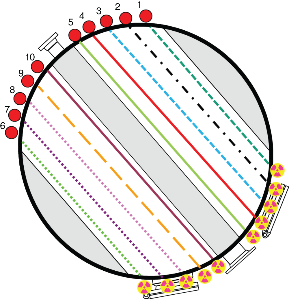
6.1.1 Harrison’s Method for Froth Height and Flood Determination
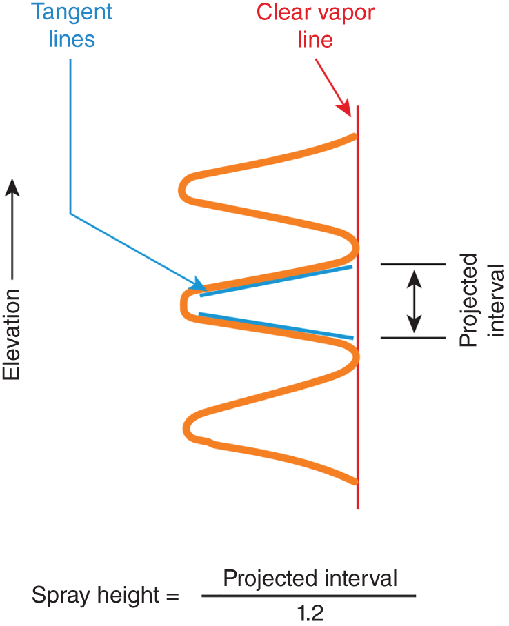
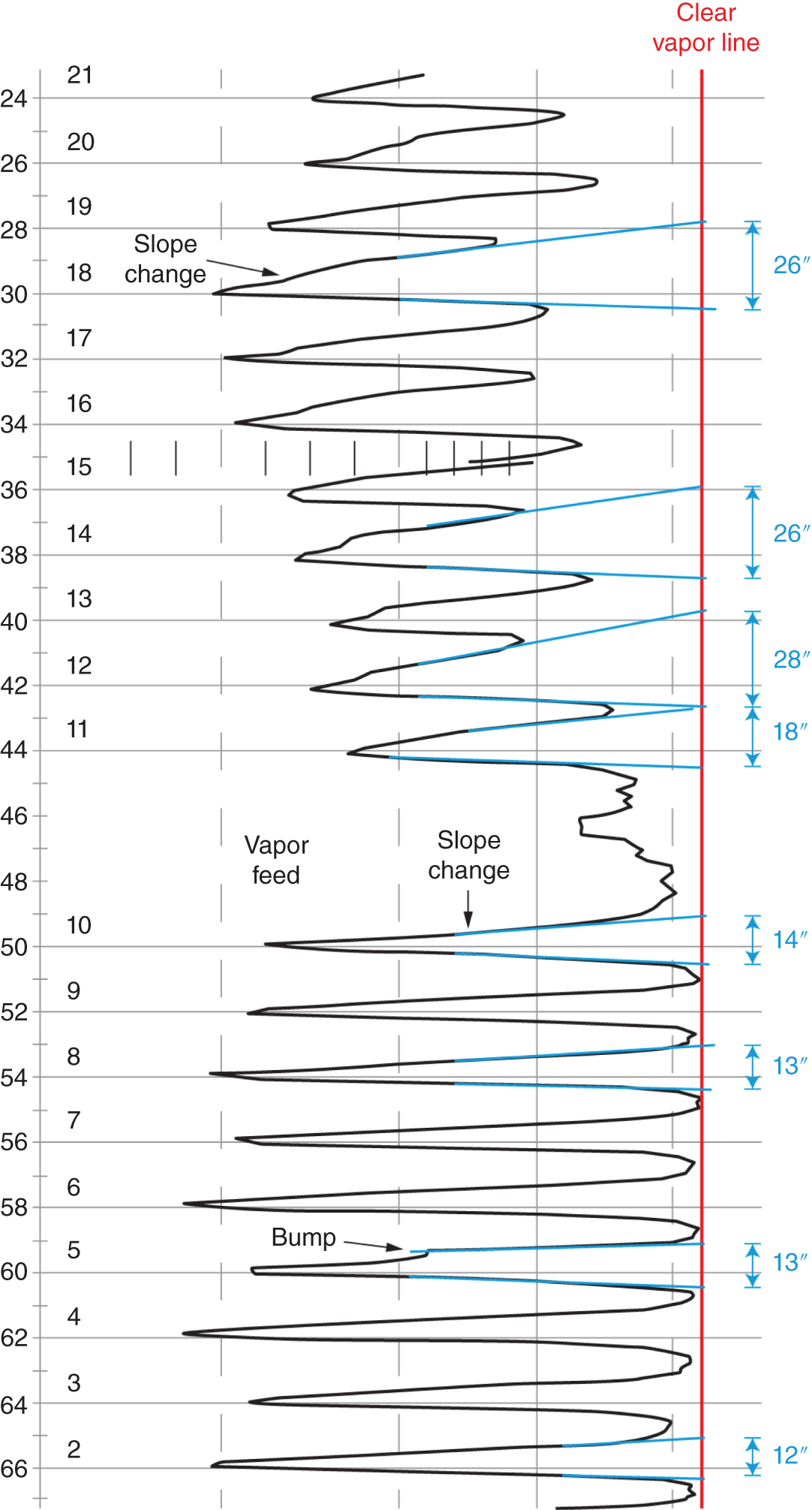
6.1.2 Application of Harrison’s Method Prevents Unnecessary Shutdown
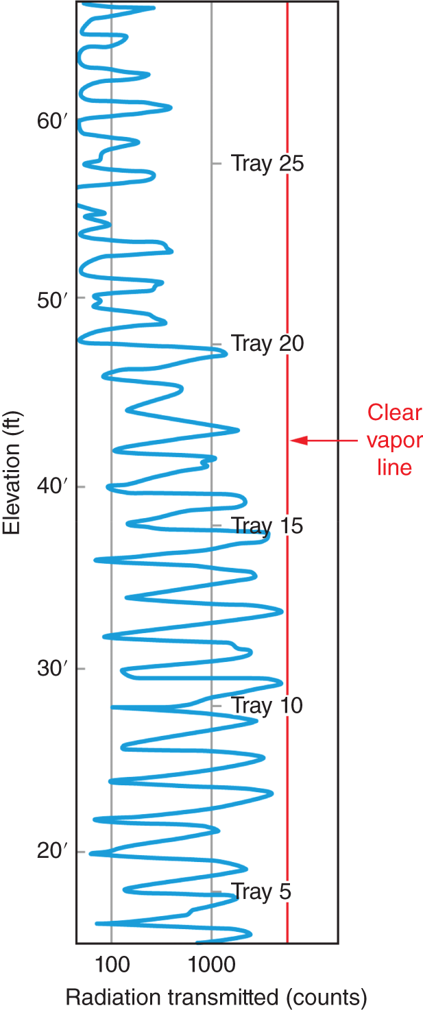
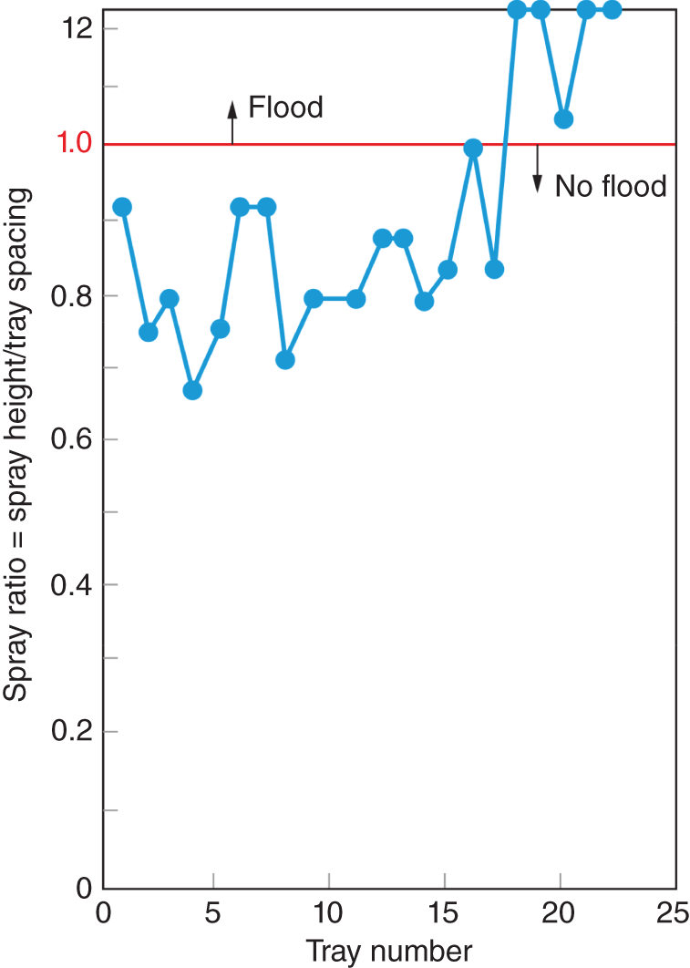
6.1.3 Entrainment Index
EI
Entrainment
>2
Flood
1.5
Heavy
1.0
Moderate
0.5
Light
0
None
6.1.4 Kistergrams and Their Application
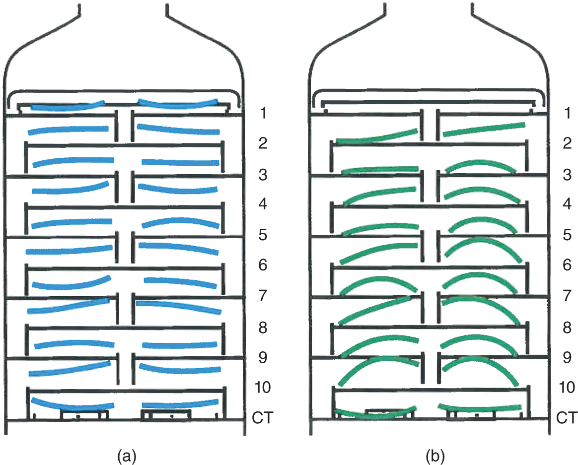
6.1.5 Froth (or Spray) Density and Liquid Head Determination
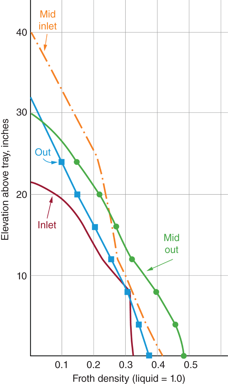
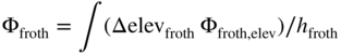
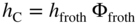
6.1.6 Quantitative Analysis for High-Capacity Trays with Truncated Downcomers
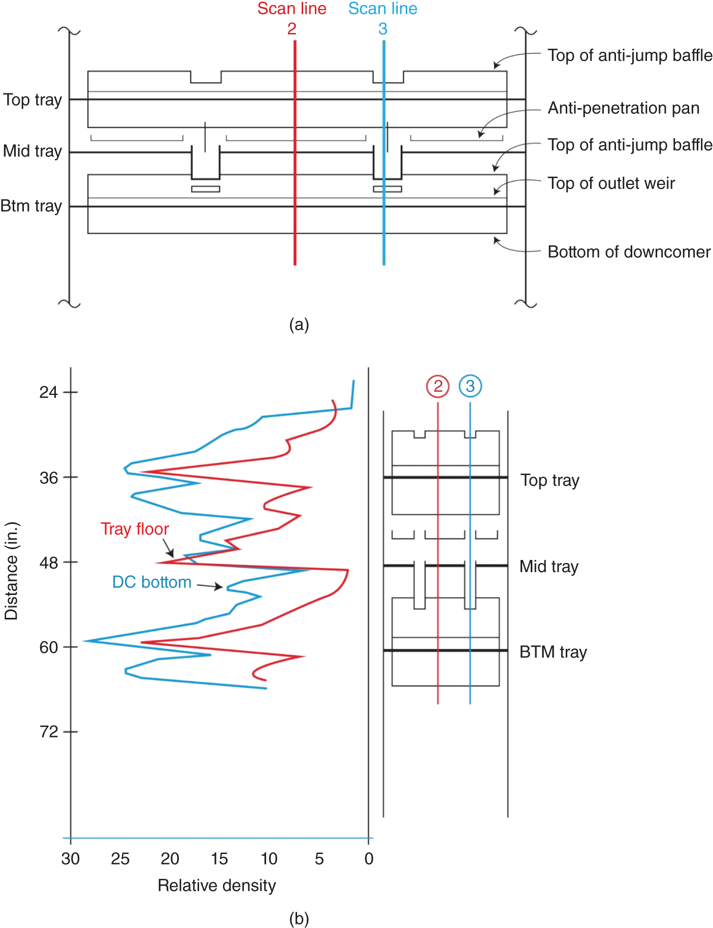
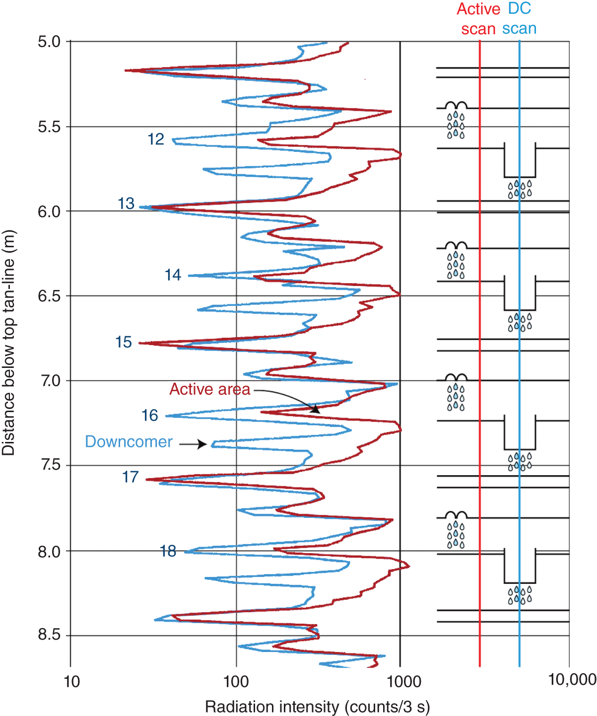
6.1.7 Scan Chord Selection
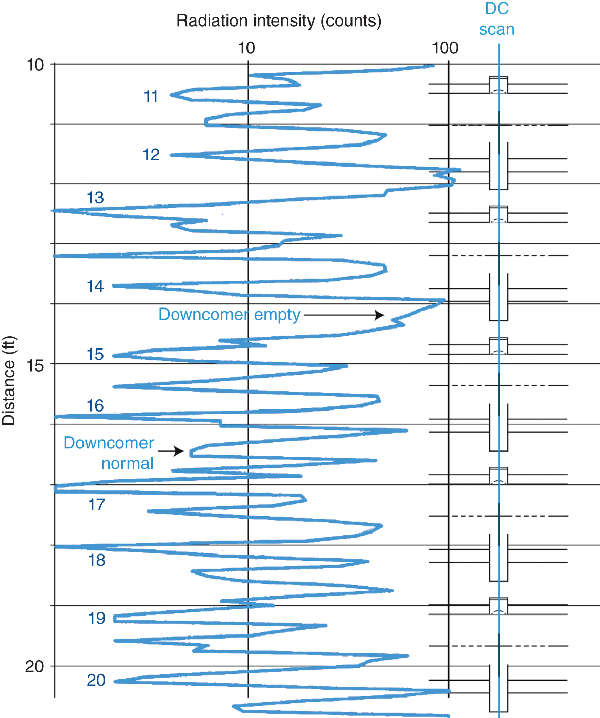
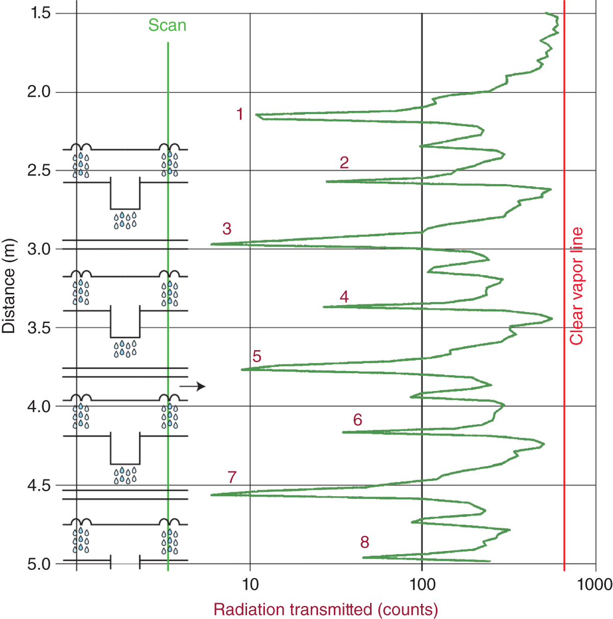

6.2 QUANTITATIVE ANALYSIS OF PACKING GAMMA SCANS
6.2.1 Packed Tower Quantitative Analysis Techniques
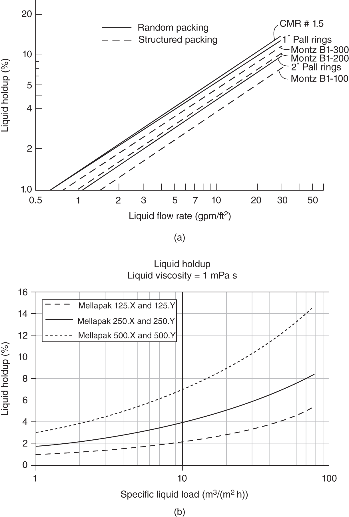
6.2.2 Flooding at the Bottom or Missing Packing Tower at the Top?
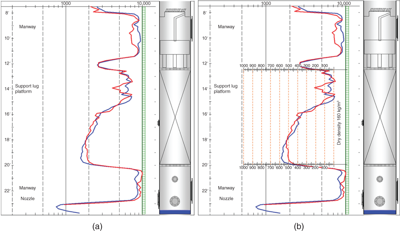
6.2.3 Dense Grid or Flooding/Coking in a Wash Bed?
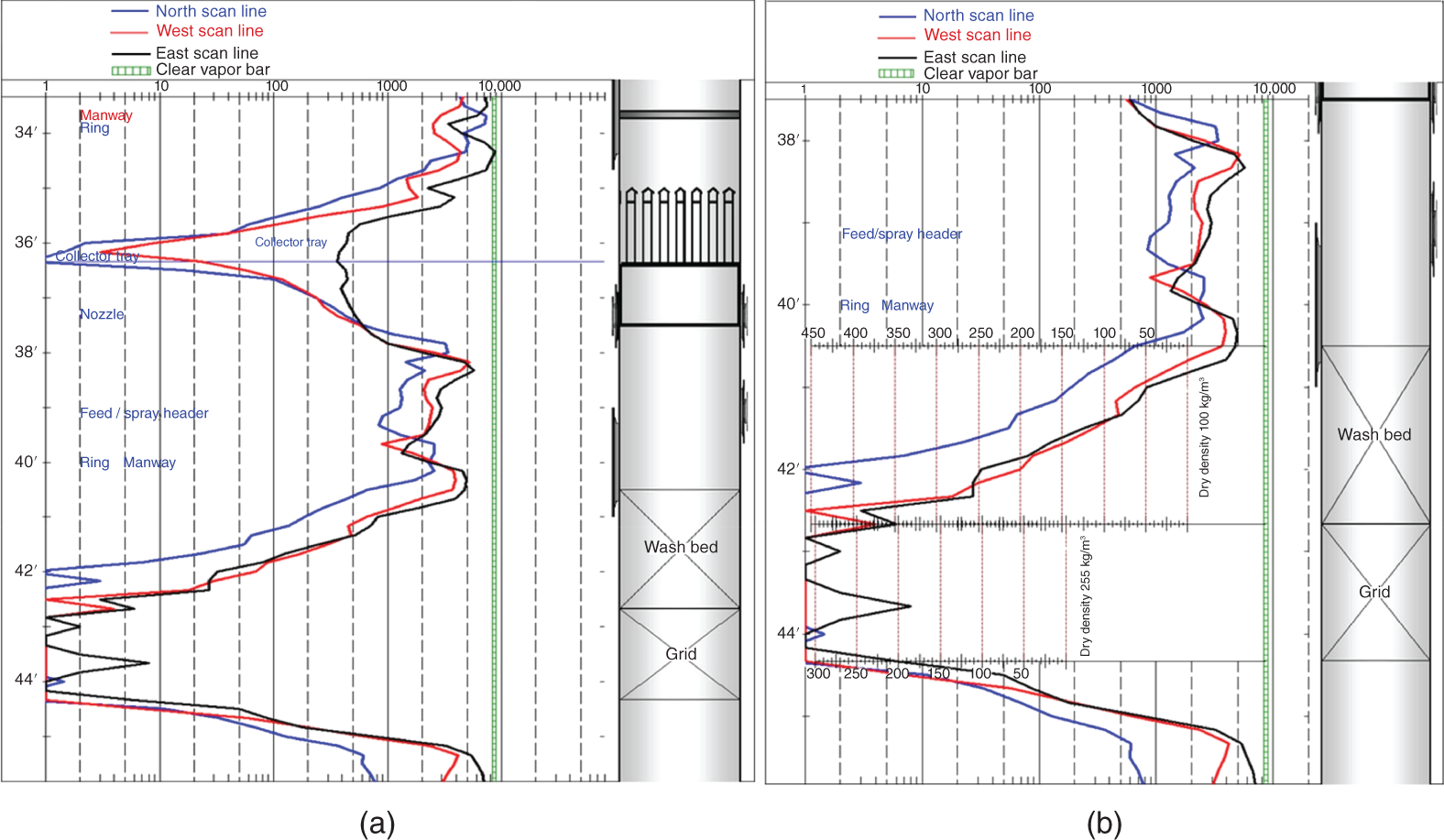
6.2.4 Good or Bad Distribution Quality?
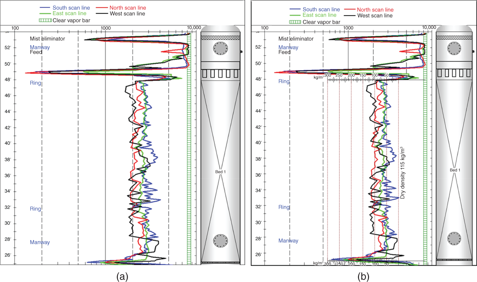
6.3 NEUTRON BACKSCATTER TECHNIQUES APPLICATION

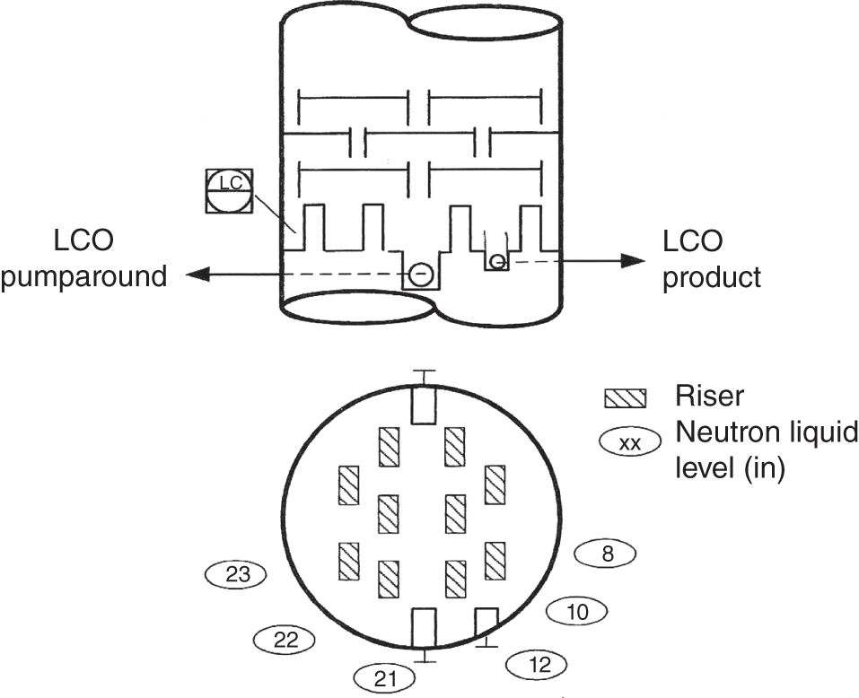
6.3.1 Detecting Flood and Seal Loss in Downcomers
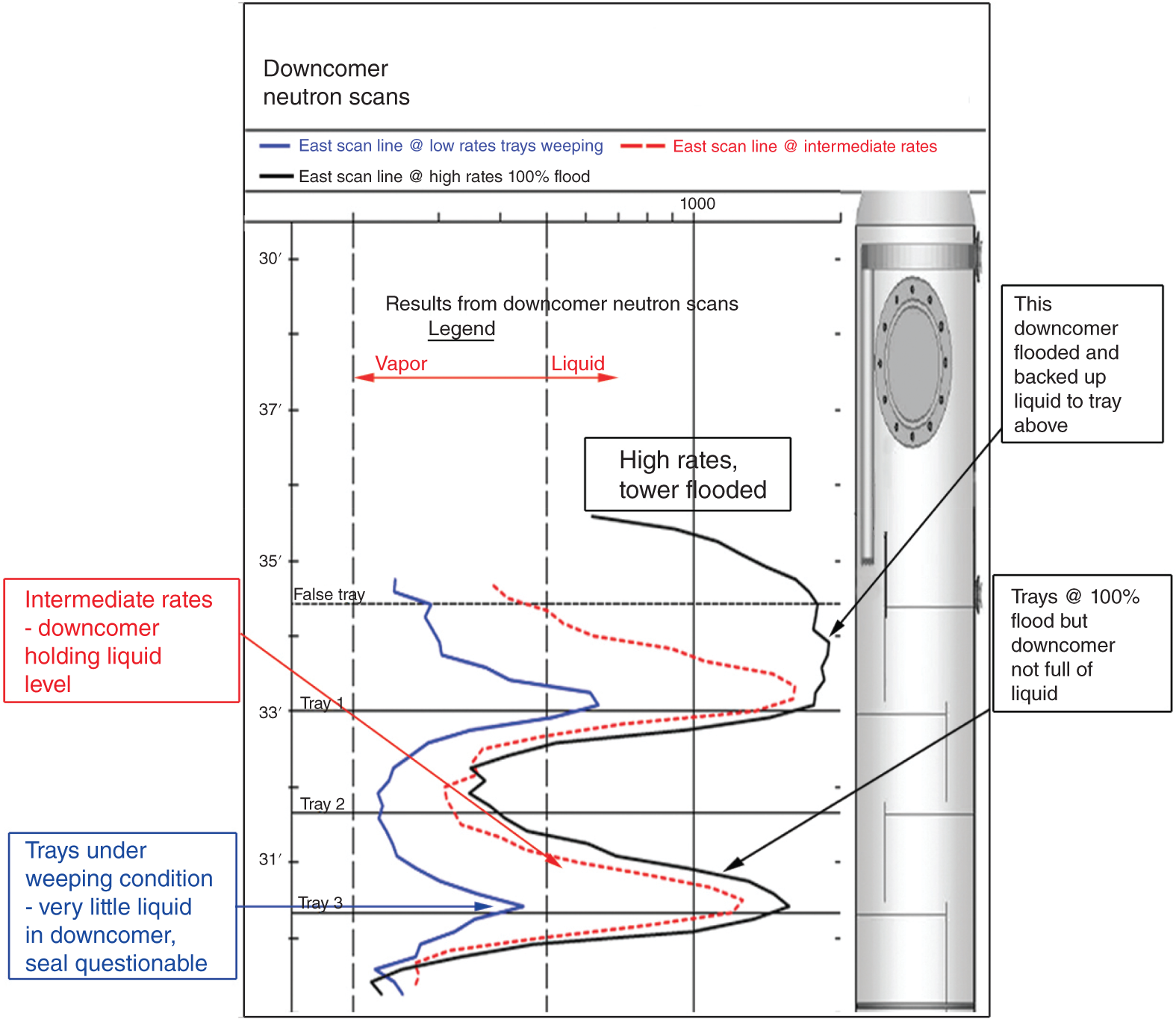
6.3.2 Distinguishing Dry from Full Downcomers
6.3.3 Detecting Maldistribution in a Kettle Reboiler

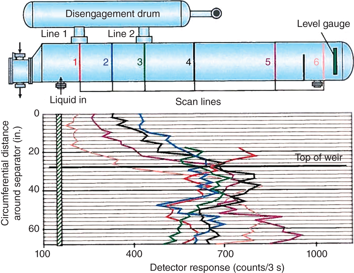
6.4 CAT SCANS
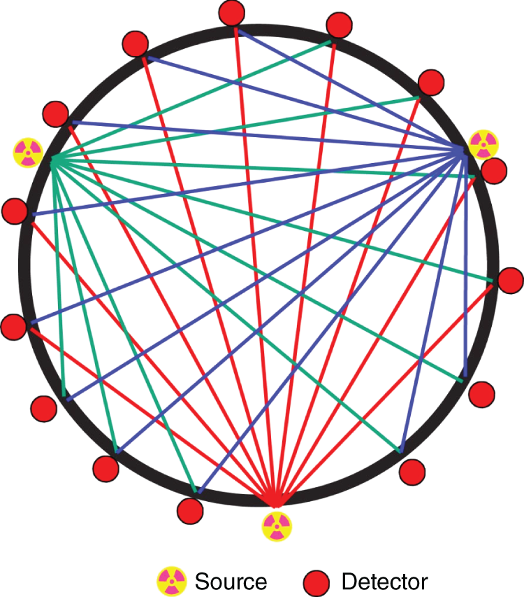
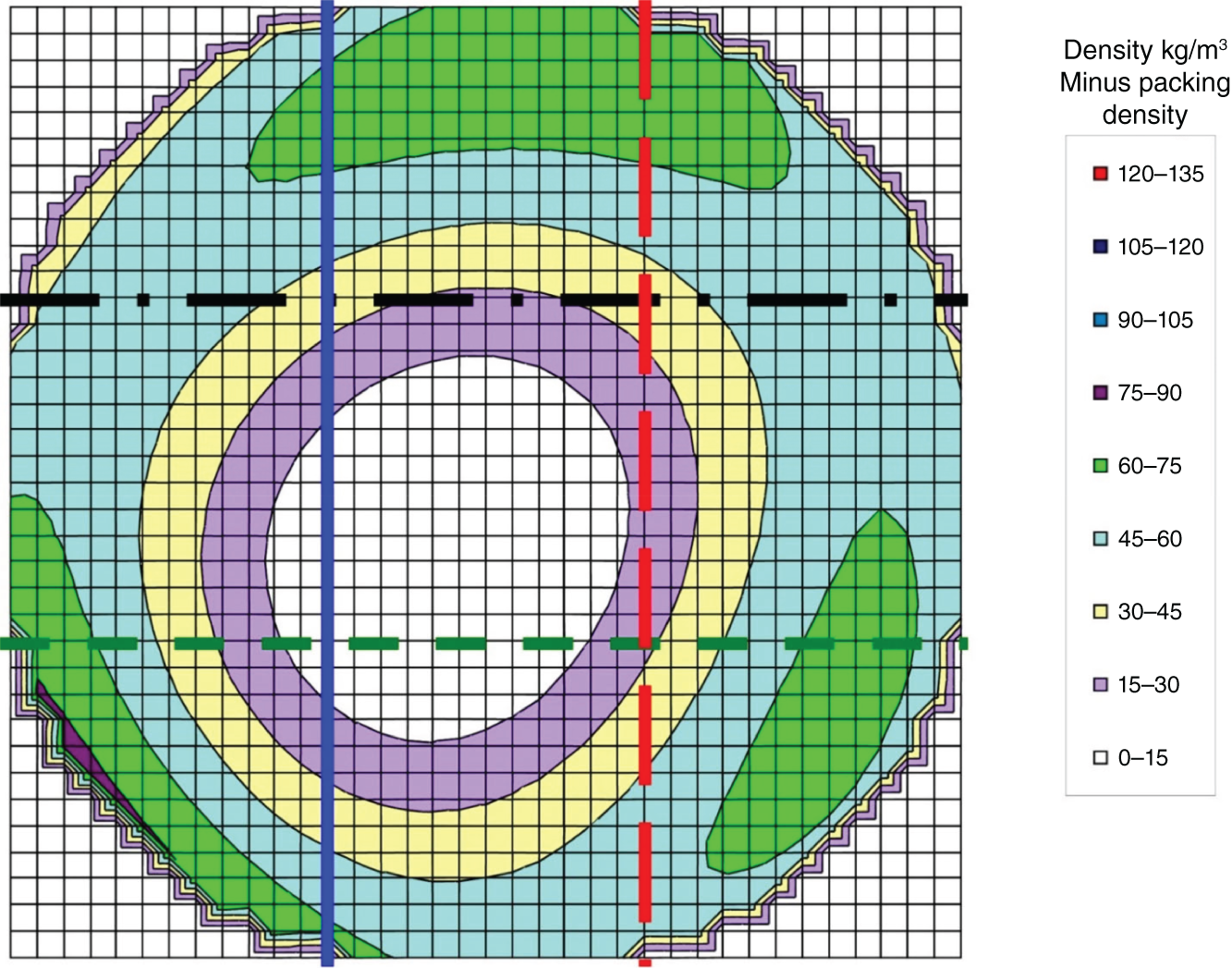
6.4.1 Identifying Unexpected Flashing in Reflux Distributor
6.4.2 Diagnosing Unexpected Parting Box Overflow
6.4.3 Monitoring Coking in a Refinery Vacuum Tower
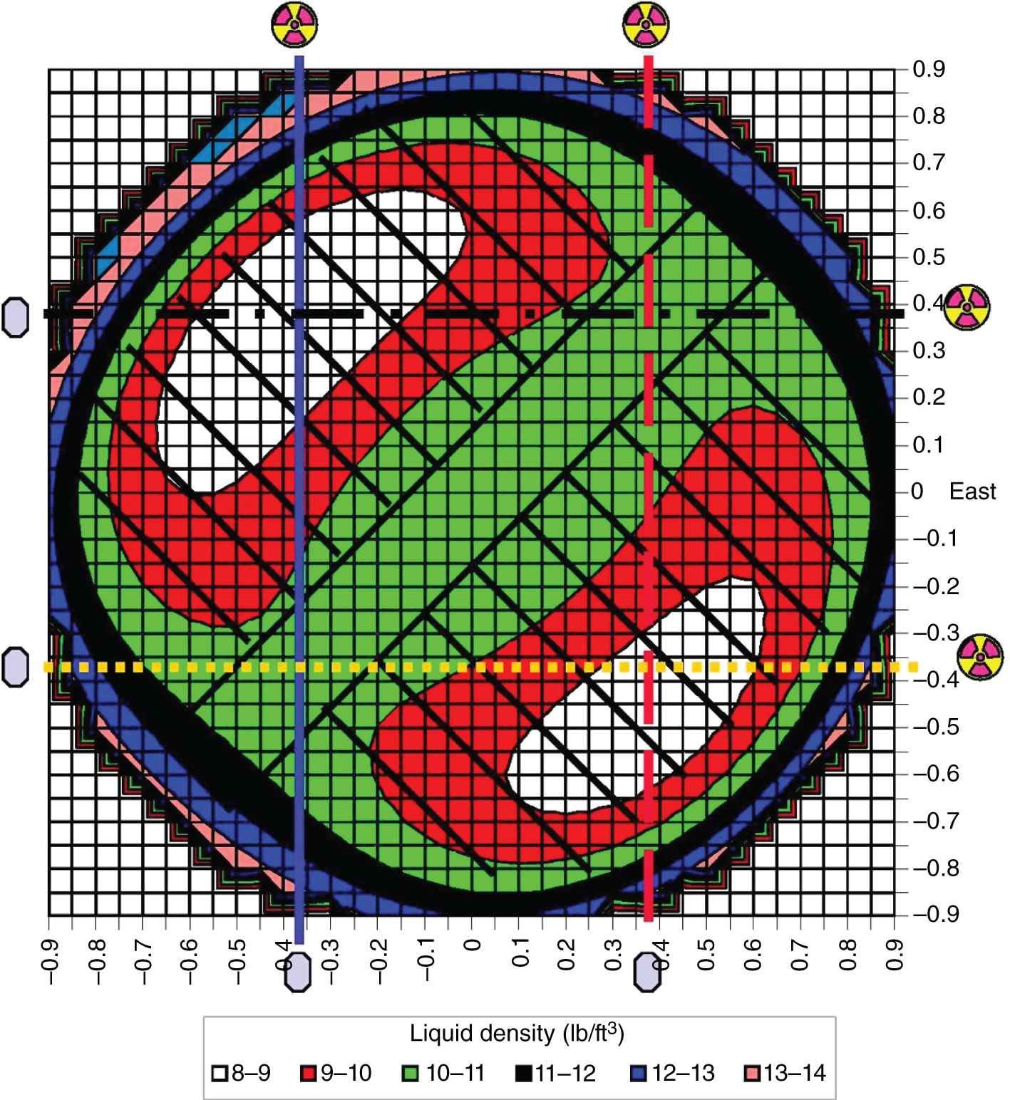
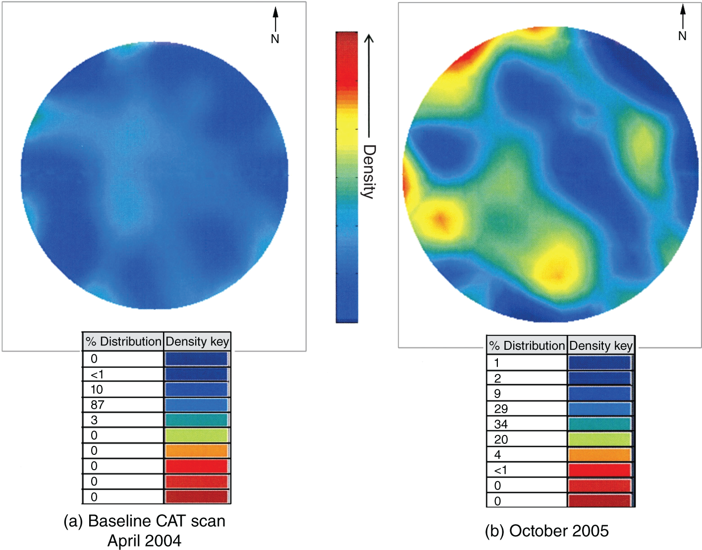
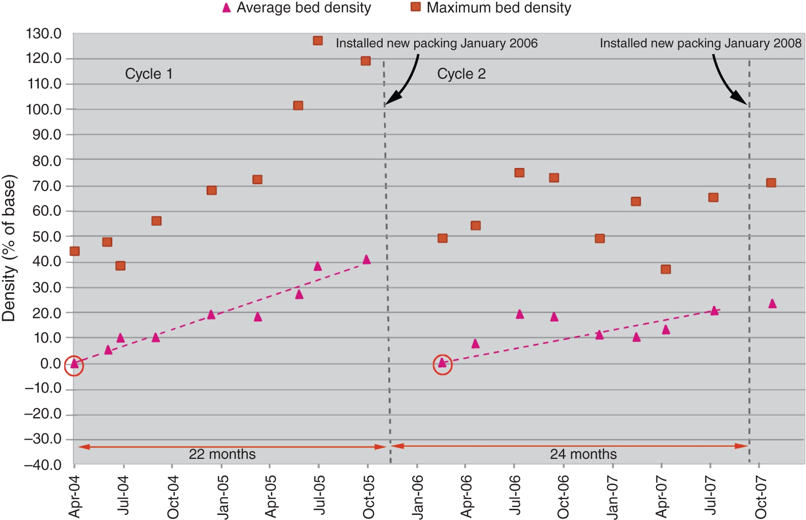
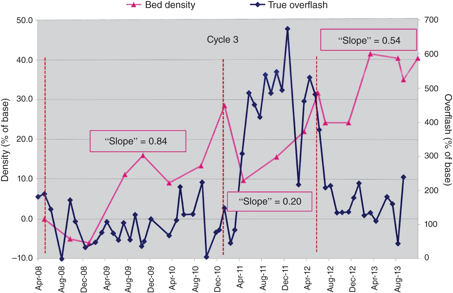
6.5 TRACER TECHNIQUES
6.5.1 Measuring Flow Rates, Internal Leaks, and Spray Entrainment in Refinery Vacuum Tower
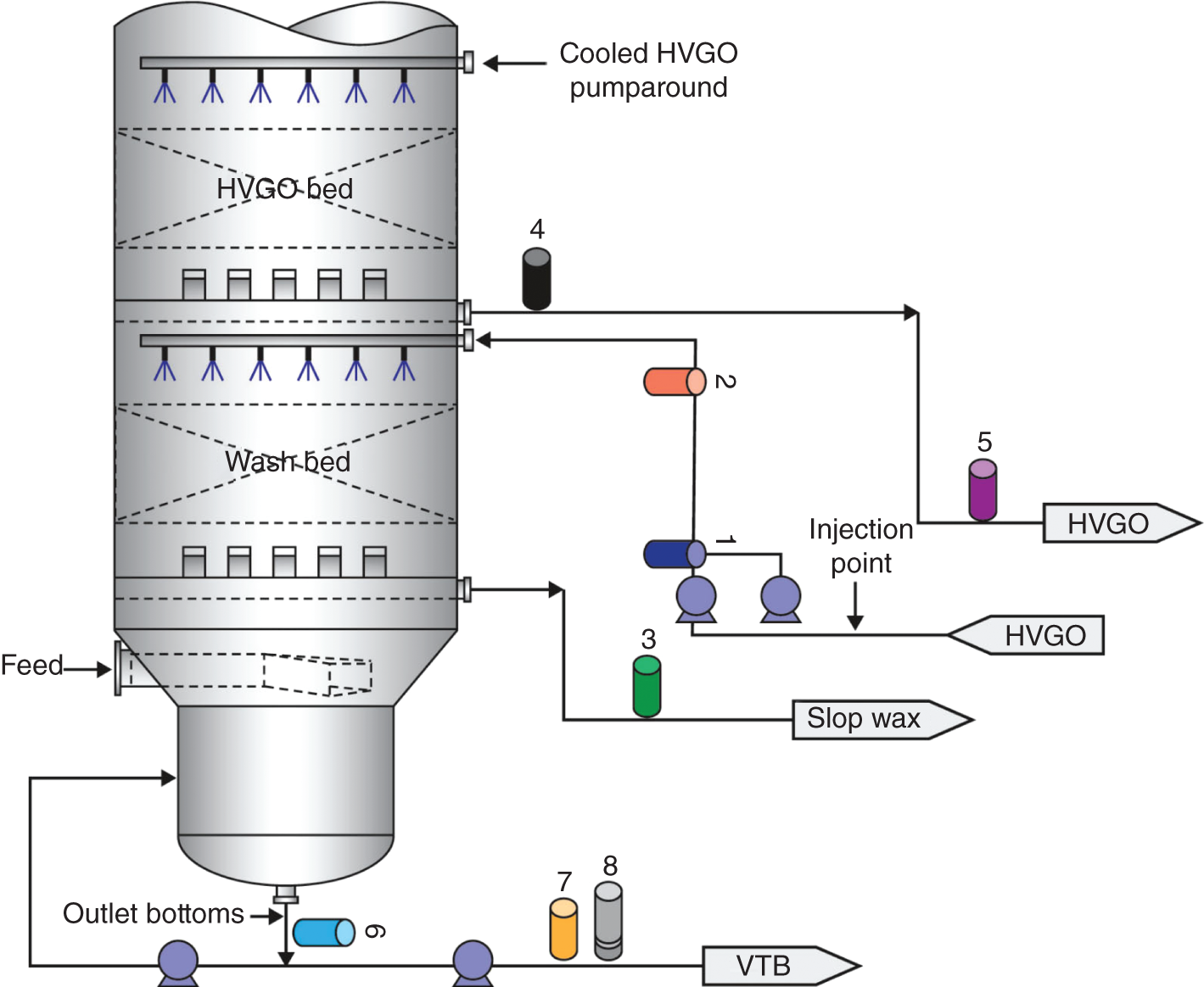
6.5.2 Observing Downward Vapor Flow in Packed Bed
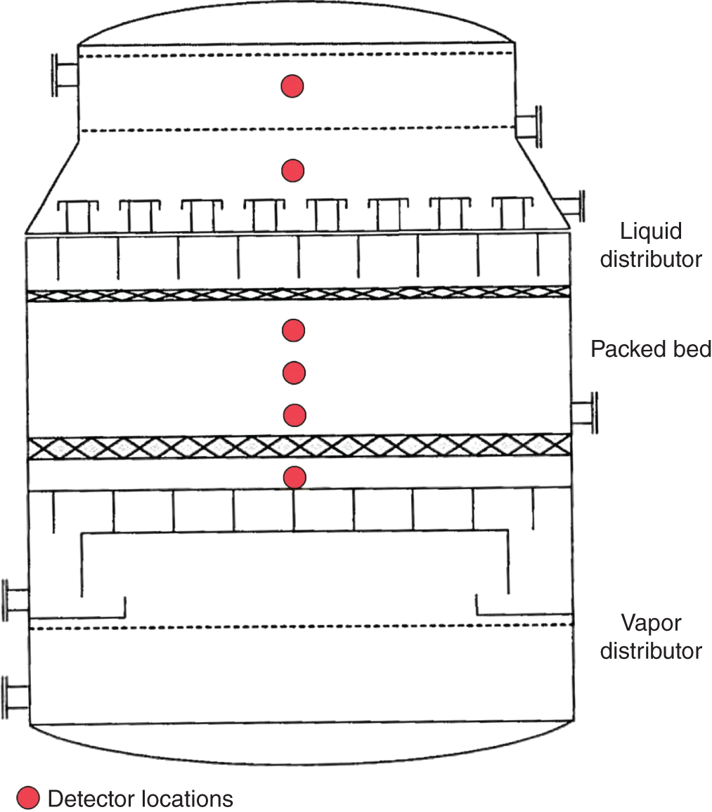
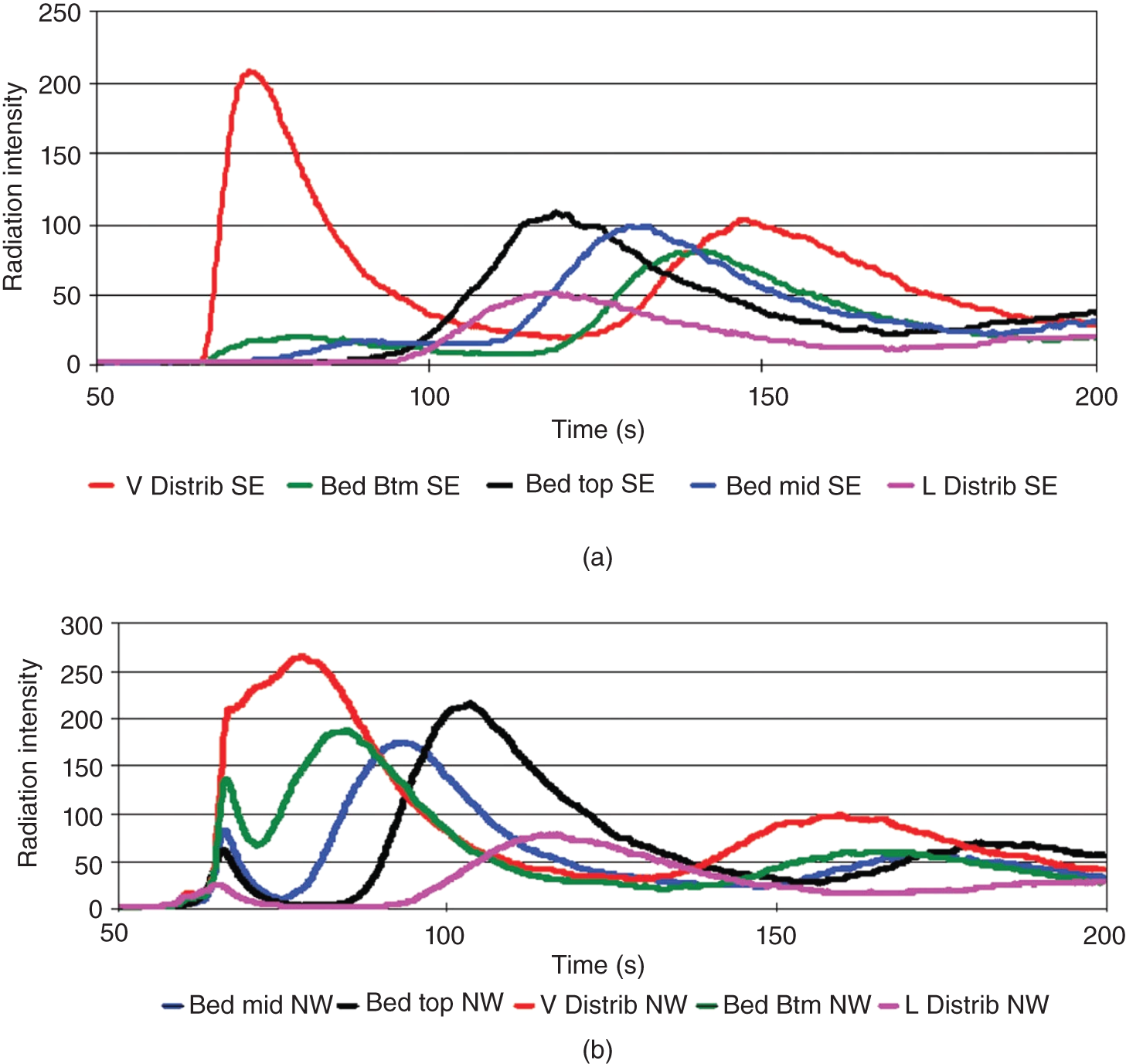
6.5.3 Quantitative Determination of Entrainment from a Kettle Reboiler
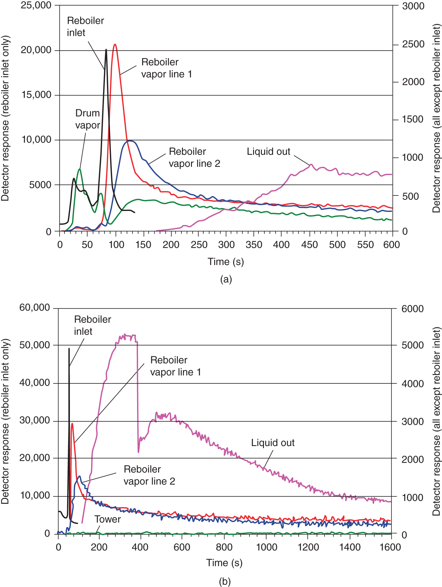

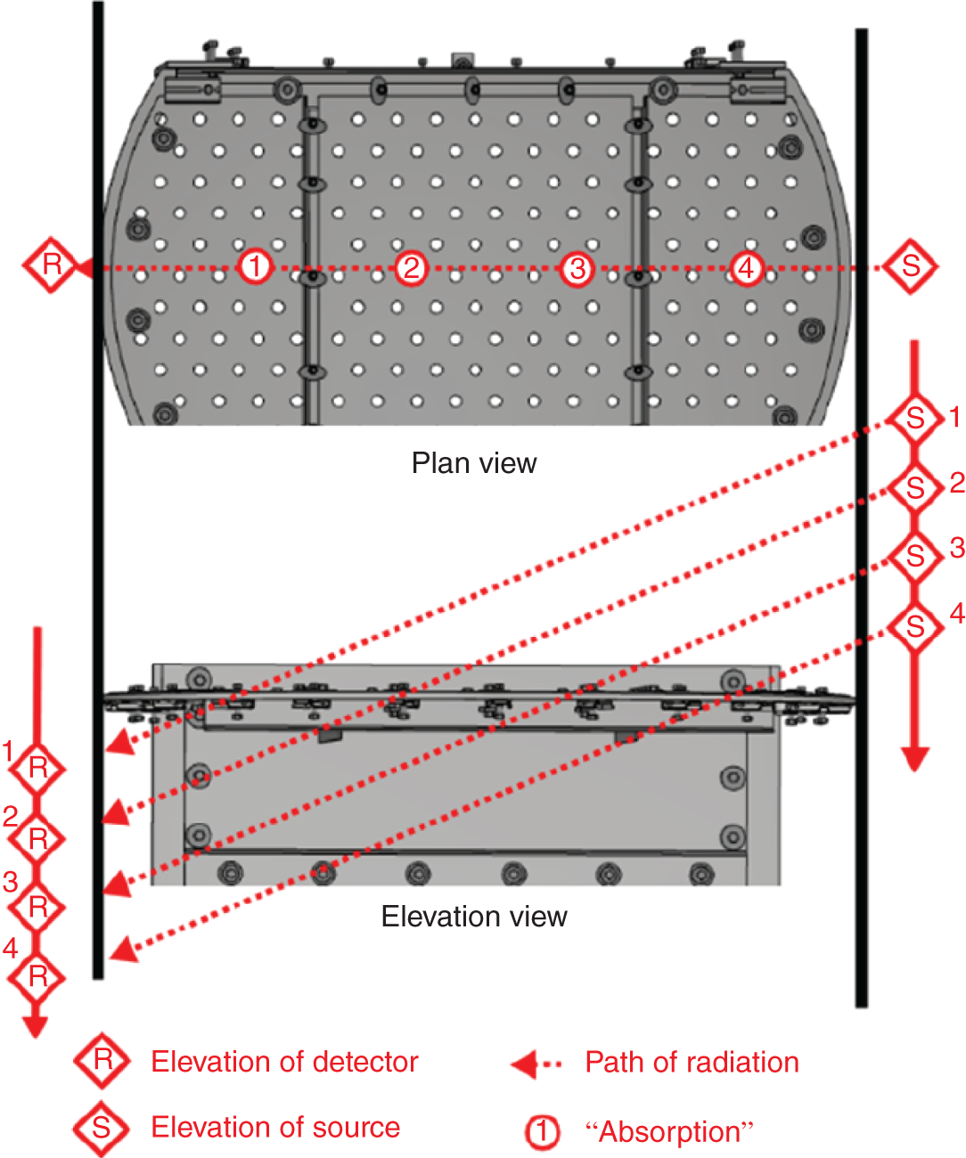
6.6 SLANT SCANNING
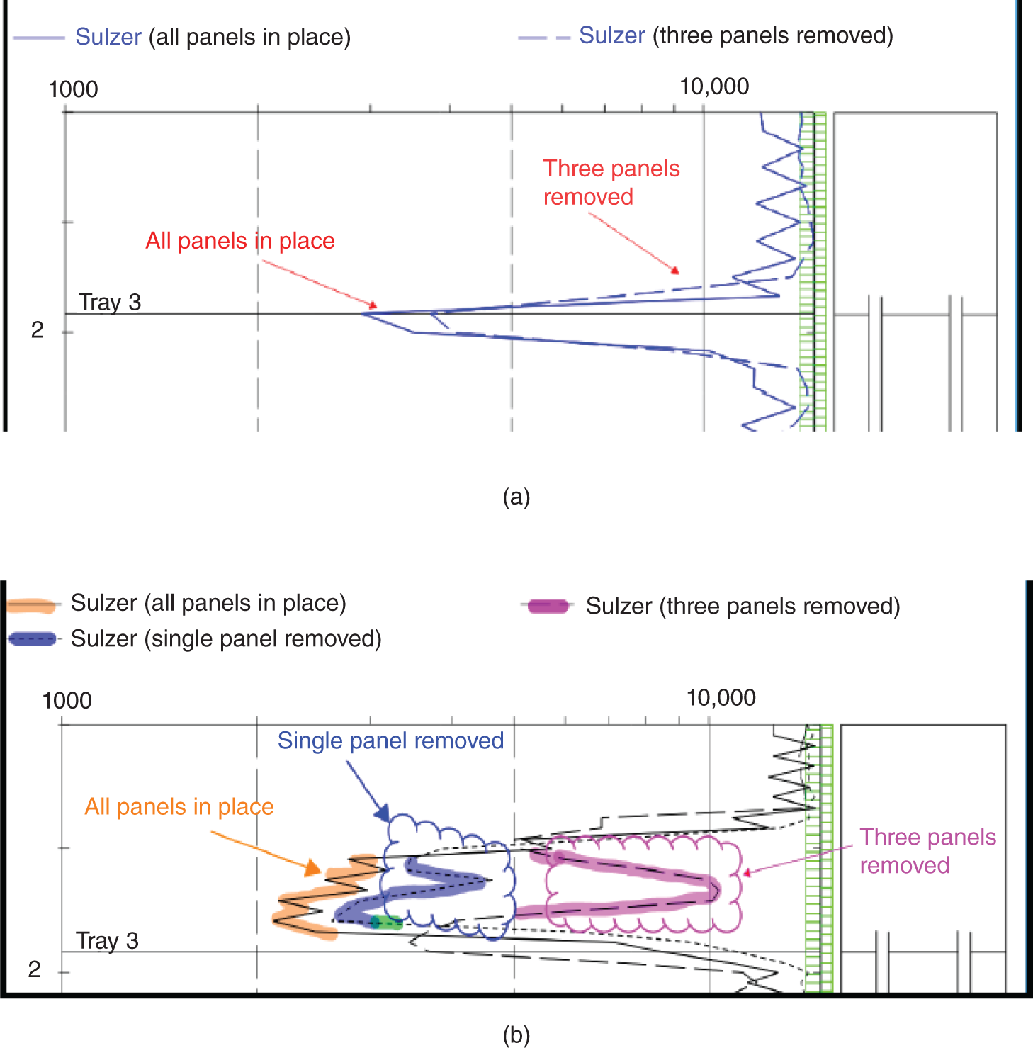
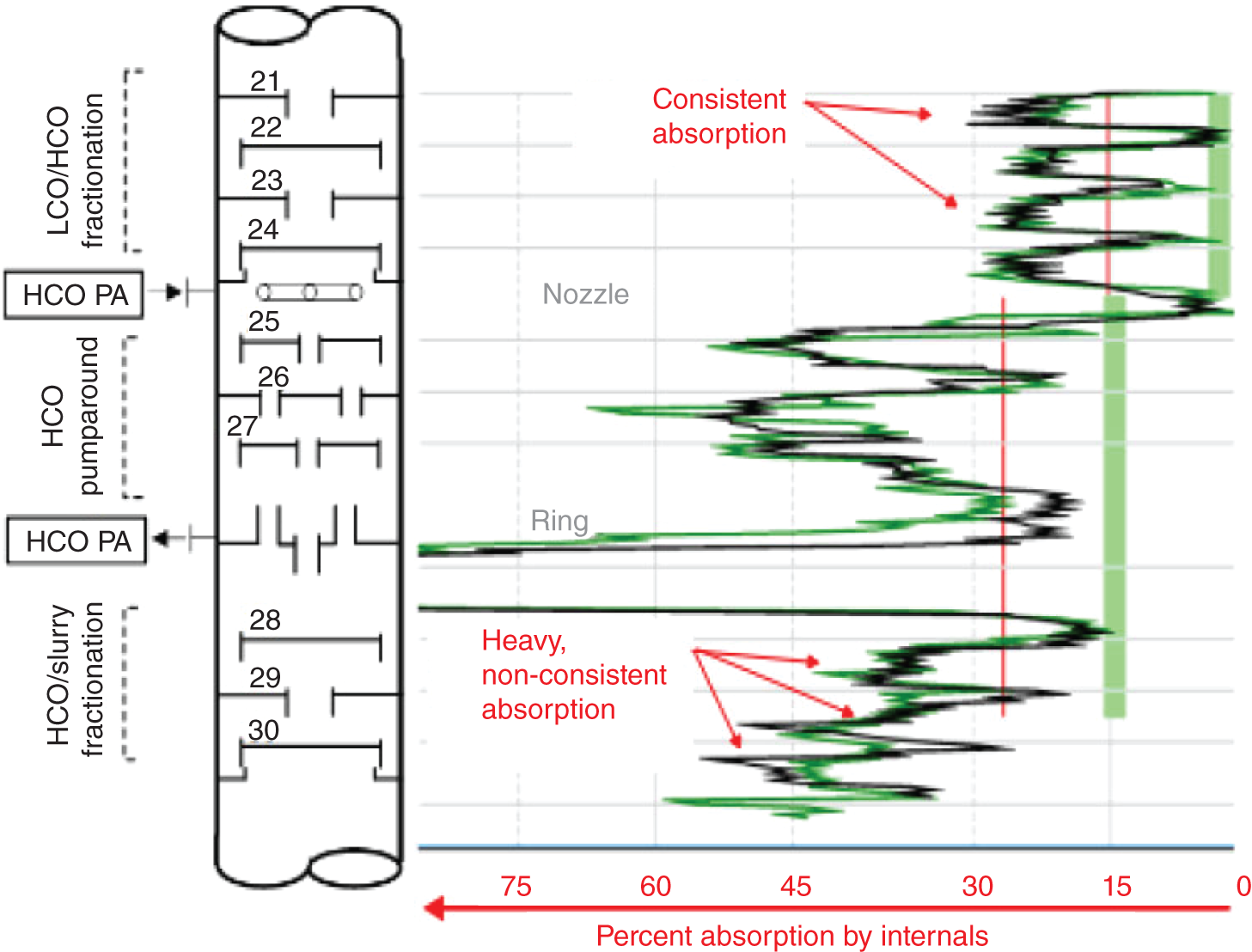
6.7 USEFUL CASE HISTORIES LITERATURE
6.7.1 Qualitative Gamma Scans of Trays
6.7.2 Qualitative Gamma Scans of Packings
6.7.3 Gamma Scans of Points of Transition and Inlet and Outlet Lines
6.7.4 Quantitative Gamma Scans of Trays
6.7.5 Quantitative Gamma Scans of Packings
6.7.6 Neutron Backscatter
6.7.7 CAT Scans
6.7.8 Tracer Technique
Advanced Radioactive Techniques for Distillation Troubleshooting

(6.2)
(6.3)

(6.5)