Petroleum has been discovered. The appraisal process is designed to determine the size of the pool and whether the petroleum accumulation should be developed. Appraisal commonly involves drilling wells and the acquisition of more seismic data. The data collected during appraisal are used to delineate the petroleum pool, to establish the degree of complexity of the reservoir, to characterize the fluids (petroleum and water), and to judge the likely performance of the field when in production. These technical assessments will be merged with economic criteria to establish whether the discovery has value and whether it can be developed commercially. The outcome of an appraisal program will either be a development program, postponement of a development decision, or abandonment of the project. If the decision is to develop the petroleum pool, then the value of the project will depend directly upon the way in which the results of the appraisal program are used to design the development. Project value is controlled by reserves, production rate, operating expenditure (OPEX), capital expenditure (CAPEX), oil (or gas) price, and transportation costs. The reservoir and trap description derived during appraisal controls initial estimations of reserves, production rate, OPEX, and CAPEX (Figure 5.1). However, the cost of appraisal is high and it must to be subtracted from the eventual value of the accumulation. Thus the petroleum geoscientist must be able to determine how much uncertainty to carry into the development program. In an ideal situation, the uncertainty in reserves defined during exploration diminishes through the appraisal, development, and reservoir management (production) phases of a field’s life (Figure 5.2). Moreover, the range of reserves at sanction (development decision) should be large enough that subsequent reserves estimates do not fall outside the range. Typically, reserves estimates fall during field appraisal as the complexity of the petroleum accumulation becomes apparent. The reverse trend is often true of the reservoir management phase. Here, a combination of dynamic data, new technology, and facilities upgrades can lead to reserves growth (Chapter 6). The importance of the appraisal program can be stressed by reference to two examples taken from the Brent Province within the North Sea. In the first example, the Magnus Field, reserves were significantly underestimated. Although the exploration department in BP (British Petroleum) had adequately captured the uncertainty in both the oil in place (550–2200 MMBO) and the reserves (220–880 MMBO), a single value for the reserves of 450 MMBO was calculated at the end of the appraisal program. The corresponding oil-in-place figure was estimated to be 1000 MMBO ± 15%. The facilities were designed and built to deliver the 450 MMBO. However, before a single barrel had been produced, the oil-in-place and reserves estimates were increased by 20%. Fifteen years after the development decision was made, the calculated oil in place was 36% higher than had been estimated at sanction and reserves were up by 61% (still within the original exploration range). Superficially, the spectacular reserves growth shown by Magnus is good news, and although such a situation is better than having to downgrade the reserves continuously, it is detrimental to project value. The facilities installed on Magnus were insufficient and the wells too few. The plateau production achieved was 155 000 BOPD. This can be compared with a plan of 120 000 BOPD. With the appropriate facilities, the rate could have been over 220 000 BOPD. Figure 5.1 The interrelationship between reserves, production rate, operating expenditure, capital expenditure, and oil price. Source: Dromgoole and Spears 1997. Reproduced with permission of Geological Society of London. Figure 5.2 Temporal changes in reserves estimation during field development and production. In the ideal situation, the uncertainty in reserves should both decrease with time and stay within the initial reserves range estimate. The Thistle Field is an example of a field for which reserves were overestimated and, as a consequence, the facility build was too large and thus too costly (Brown et al. 2003). Sanction for the field development was obtained in 1974. At that time, the pool had been penetrated by only three wells and seismic coverage was limited to a 2D data set. Oil in place was estimated at 1350 MMBO. By 1992, the oil-in-place figure had been recalculated to be 820 MMBO. The corresponding reserves figures were 490 MMBO and 410 MMBO. The spectacular reduction in oil in place was not completely reflected by the decline in reserves, because it had proved possible to raise recovery from 36% to 50%. This increase in the recovery factor was achieved although the reservoir proved to be far more complex (segmented) than had been appreciated at sanction. However, many infill wells were required to deliver the increased recovery. In this chapter, we examine the geoscience components within the process of appraisal. It will be clear to the reader that the scale and range of observation change from exploration to appraisal. No longer is the geoscientist concerned with the presence and maturity of the source rock or the risk of migration, for the petroleum accumulation has been found. However, the ellipsoidal bump that proved an adequate description of the trap at the exploration stage is no longer sufficient. A detailed description of the trap envelope and its contents, the reservoir and petroleum therein, is needed. Sections 5.2–5.4 examine the definition of the trap envelope in terms of the bounding surfaces (fluid contacts and trap geometry) and internal segmentation. In Sections 5.5 and 5.6, we further analyze the reservoir architecture and reservoir characteristics on a pore scale. The theme of reservoir description is developed in Section 5.7, where the utility of seismic data is explored. The primary product of the appraisal program is an estimate or range of estimates of oil and gas in place based upon the appraisal data. These data, together with reservoir architectural and a few dynamic data, are then used to populate a reservoir model (Section 5.8). The two case histories are taken from Venezuela and South Asia. The example from Pakistan concerns a field discovery which, during the appraisal phase, was assessed to contain almost a trillion cubic feet of gas reserves but when the first development (production) well was drilled it was dry, the reservoir having been penetrated below the gas water contact. The appraisal program had failed to identify the key uncertainties. The case history from Venezuela concerns a field that was re-appraised 60 years after first having been discovered and produced. The appraisal program failed to identify highly viscous oil within a sizable part of the field and hence was far too optimistic in terms of reserves and producibility. Much of the data that we use to describe the subsurface – whether it be for appraisal, exploration, or production – are derived from seismic. Moreover, such seismic data are often displayed using two-way time, not depth, for the vertical axis. In making geologic interpretations using conventional seismic displays, we make a mental assumption that two-way time and depth are positively and simply correlated. In gross terms, this assumption is true on most occasions (Figure 5.3). The interpretation of geologic structures and geometries on normal seismic sections is perfectly valid. However, it is important to be aware that on some occasions the Earth’s velocity field is not constant at a given depth. In consequence, obvious structures in the time domain may not exist in the depth domain, and real structures in the depth domain may not exist in the time domain and thus be invisible on seismic data The gross assumption that two-way time and depth are positively and simply correlated is also commonly inadequate for the purposes of well prognosis, well engineering, and evaluation of petroleum volume in a trap. In order to make each of these calculations, it is necessary to convert time to depth. The aim of this section is to examine what data are used in this process, the various methods that can be employed, the resultant uncertainties, and their effects upon the way in which the subsurface structure is interpreted. Quite clearly, the relationship between depth and seismic two-way travel time is the velocity of seismic energy in the subsurface. The velocity is controlled by the mineralogy of the rock, the state of cementation, the pore fluid, and the porosity fabric. The seismic velocity is greater in well-indurated rocks such as limestone and dolomite compared with most sandstones. Soft sediments such as muds and coals are particularly “slow.” Rock with fluid-filled pores transmits seismic energy more slowly than nonporous rock, and petroleum-filled pores reduce velocity more than water-filled pores. Small quantities of gas can cause dramatic velocity reductions. The pore fabric is also important; for example, a low-porosity but fractured rock commonly has a lower-velocity transmission than a rock with the same primary porosity. This is because the fracturing weakens the fabric of the rock and lowers its elasticity. Figure 5.3 Time versus depth data for wells within the Inner Moray Firth, UK North Sea. The data are from check shot surveys in each of the wells. This curve would be used to convert a two-way time map derived from seismic data into a depth map. The degree of sediment compaction and cementation commonly increases with depth, and as a consequence seismic velocities commonly increase with depth. Exceptions to this generality occur within zones of fluid overpressure (Chapter 3). In such situations, the fluid supports part of the lithostatic load, porosity is often relatively high, and thus fluid content can be high. Consequently seismic velocity can be lower in overpressured intervals than in similar hydrostatically pressured intervals. It is clear from the above paragraphs that heterogeneity in the lithology distribution, fluid distribution, and pressure (overpressure) distribution will cause heterogeneity in the velocity field. Such velocity heterogeneity needs to be understood to make a detailed conversion between two-way time and depth. The data used for depth conversion come from one or more of four sources: calibrated sonic logs, pseudo-velocities, stacking velocities, and regional knowledge. Pseudo-velocity is the term used to describe velocity data calculated from combining well depths with seismic arrival times. Velocity data may be calculated for a point (from a sonic log), as an average for an interval or as the average from the Earth’s surface (Tearpock and Bischke 1991). Such velocity data may then be used to convert to depth using one or more of a time–depth curve, an average velocity calculation, a layer cake conversion, or ray tracing. An average velocity calculation uses a simple algorithm for a whole well (Figure 5.4a). No attempt is made to incorporate systematic variations in velocity that can occur with depth. The technique is often applied when wells are without sonic logs, check shot data, or vertical seismic profiles (VSPs), or when such data are of suspect quality. In the interval velocity method for time-to-depth conversion, the geology represented on the seismic section is divided into its constituent layers (sequences). The average velocity for each layer is then calculated and the resultant layer cake of interval velocity data used to make the conversion (Figure 5.4b). Figure 5.4 A synthetic sonic log for a well, showing three possible methods for calculation of velocity profiles that can then be used for depth conversion of seismic data. (a) The average velocity model; (b) the internal velocity model; (c) The instantaneous velocity model. The instantaneous velocity model (Figure 5.4c) represents an improvement on the interval velocity method and can be used when velocity data from Check shots or VSPs are more abundant. Ray tracing is commonly used to check the validity of time-to-depth conversions. The method uses the generated depth maps and velocity data to generate a synthetic seismic section. The generated section is compared with the real seismic data. If the match is poor, the input data are readjusted until an acceptable match is obtained. The refined input data may then be used for time-to-depth conversion elsewhere in the area of interest (McQuillan et al. 1979). Subsurface maps are a fundamental part of petroleum geoscience. They are used at all stages of exploration, appraisal, and development. Regional geologic maps were examined in Chapter 3, and the use of structural maps to interpret petroleum migration and prospectivity was covered in Chapter 4 (including the case histories). We choose to study mapping more closely in this chapter because at the appraisal stage the need for accurate and reliable maps increases disproportionately relative to the data available. Many of the criteria that are used to determine whether a petroleum pool will be developed or abandoned without development will be based upon subsurface maps, and yet the quantity of data available is likely to be limited to a few wells and a 2D or 3D seismic survey. Maps can be produced for both surfaces and intervals (or their properties). Here, we look at surfaces. Intervals and interval properties are examined later in this chapter (Section 5.8), although the methodology for construction of the surface and interval maps is similar. Maps are most commonly constructed on stratigraphic (iso-geologic time) surfaces. These may be either conformable surfaces or unconformities. Time-slice extractions from seismic data are also maps, and these can also form the basis for structural and stratigraphic interpretations. It is also possible to produce maps on fault surfaces. In such instances, it is common to plot the intersection of the stratigraphy on the fault surface for both the footwall and hanging-wall surfaces. Cross-sections can also be constructed from maps. The construction of cross-sections can further aid the interpretation of both structure and stratigraphy. Both structural and interval maps are 2D representations of 3D data. The elevation, thickness, or property data are commonly portrayed as contours. Contours are lines that connect points of equal value. Relative contour spacing conveys much information about the properties of a surface (Figure 5.5). Equally spaced contours indicate that a surface has constant slope (dip). Closely spaced contours indicate a more steeply dipping surface than more widely spaced contours. Therefore, in producing a map from point source well data or from seismic data, care must be taken during the contouring process to ensure that the map accurately conveys the interpretation intended. There are a few important rules to consider when producing a contour map. A contour line cannot cross itself. It must also form a closed surface (although this may be beyond the bounds of the map). Contours appear to merge on vertical surfaces and appear to cross on overhanging surfaces, but in 3D space the contour lines lie one above another. To avoid confusion, contours on overhanging surfaces are commonly shown dashed (Figure 5.6). Repeated contour lines of the same value indicate a change of slope (synclinal or anticlinal culmination; Figure 5.7). Figure 5.5 The spacing of contour lines is a function of the shape and slope of the surface being contoured. Source: Adapted from Tearpock and Bischke 1991. Figure 5.6 Contours on the underside of an overhanging structure (a) are shown as dashed on a map (b) so that they are clearly different from those on the upper surface. The contours shown here are in feet. Source: Adapted from Tearpock and Bischke 1991. Tearpock and Bischke (1991) provide a simple guide to contouring, to enable easy construction and subsequently easy understanding by the reader. They suggest the following: Figure 5.7 A sketch of a mapped surface, showing anticlinal, and synclinal culminations. Repeated contours at the crest of the anticline and trough of the syncline demonstrate the change of slope. For maps produced from 2D seismic data, the data density is commonly greater than that produced solely from well data. Elevation data (two-way time) are transferred from lines interpreted on the seismic section onto shot point maps. In situations in which 3D seismic data are being interpreted, the data density is commonly so large that the map essentially makes itself as the geologic surfaces are interpreted. Indeed, on most workstation software it is possible to pick every 10 or 20 lines in a 3D seismic volume and then “zap” the surface. In this process, the software automatically picks the same reflectors on adjacent lines. In structurally complex areas such automatic picking may break down, since the continuity between lines is insufficient. With such a high density of data, it is commonly possible to produce a map with a similar level of detail to many topographic maps. Moreover, the high density of data may also allow mis-picked surfaces to be easily identified. Computer-aided contouring can suffer from the same problems as hand contouring, although because the choice of algorithm (method) is not always readily apparent to the operator, the detection of errors is rarely easy. Faults are commonly an important part of overall trap geometry and internal segmentation of a petroleum pool. Care must be taken in construction of the fault surface, because the interpreted position of the fault will control the calculated volume of the trap or field segment. Care is also needed to define accurately the position of a fault surface from the perspective of drilling wells. Since faults are commonly boundaries within fields, wells are often drilled close to them. Production wells are commonly drilled close to fault block crests (Yaliz 1997) and injection wells for gas or water can be drilled at crestal or flank limits. A well drilled on the wrong side of a fault can be a massive waste of money. A detailed analysis of fault construction, fault balancing, and section restoration is beyond the scope of this book. For this, the reader is referred to Suppe (1985). Here, we will examine fault nomenclature, fault surface maps, and the representation of faults on (stratigraphic) horizon maps. The components of a fault system are shown in Figure 5.8. The footwall of a fault is the volume beneath the fault surface and the hanging wall is the volume above the fault surface. This nomenclature holds for both normal and reverse faults. The vertical separation (B–C) is the vertical component of the bed displacement, measured as the vertical difference between the projections of a marker horizon on either side of the fault onto that vertical plane. The vertical separation is what is measured in vertical wells and on vertical cross-sections. The missing section (or repeated section for a reverse fault) is called the “fault cut” when measured vertically. The “fault throw” (B–C) is the vertical component of the dip slip (B–D). The “fault heave” (C–D) is the horizontal component of the dip slip, measured orthogonal to the strike of the fault. For maps constructed on stratigraphic surfaces, fault heave appears as gaps in normally faulted terrain (stippled in Figure 5.9) and as overlapping surfaces in reverse-faulted terrain. It is particularly common to find maps in which the gaps and/or overlaps have been ignored. Quite clearly, in these instances the geologist constructing the map has misrepresented the extent of the formations on either side of the fault surface and, by extension, has also misrepresented the volume of rock to either side of the fault. Representation of reverse faults is also problematic in much of the current generation of geocellular modeling software (Section 5.8). When using such software, it is often necessary to construct a separate geocellular model to either side of a reverse fault, to capture accurately the volume and true extent of both the footwall and the hanging wall. To mitigate the shortcomings of such software, some geologists will choose to make their reverse faults vertical and produce a single geocellular model. Naturally, this compromises the volume calculations. Moreover, such a model cannot be used for well placements. Figure 5.8 Fault nomenclature. AB, strike-slip; BD, dip-slip; BE, oblique slip; CD, heave; BC, throw; θ, dip of fault; α, hade of fault. Figure 5.9 Fault heaves appear as gaps for normal faults. This example is from the Hibernia Field, offshore eastern Canada. Source: Mackay and Tankard 1990. Reproduced with permission of American Association of Petroleum Geologists. Fault surface maps are most commonly constructed to enable examination of the relative positions of sealing horizons and reservoir horizons on either side of the fault plane. Such Allan diagrams (Figure 5.10) that is, cross-fault fluid communication, e.g. allow analysis of potential fault seal mechanisms and determination of spill points (Figure 5.10). The spill point of a structure is the deepest closed contour on that structure. Spill points define the vertical limit of the trap. The volume of rock above the spill point is within the trap and that below the spill point is outside the trap (Figure 5.11). Knowledge of the spill point for a particular trap will enable the vertical closure of the trap to be calculated. Thus spill point identification is an important part of petroleum field definition and ultimately calculation of petroleum in place. Figure 5.10 (a) A block diagram showing folded and faulted reservoir intervals A and B. The hanging wall is shown with two displacements, H1 and H2. (b) An Allan diagram showing the intersections of the reservoir intervals A and B from both the footwall and the hanging wall on the fault plane for displacements H1 and H2. The reservoir intervals are juxtaposed across the fault plane for displacement H1 (shaded). Fluids could flow across the fault plane at the points of contact between the reservoirs. The displacement H2 is too great for the reservoirs to be juxtaposed. Figure 5.11 Closing contour on Tertiary Structure Block 9/28 – South Viking Graben. Source: Courtesy of Jim Henderson. (See color plate section for color representation of this figure). Figure 5.12 Spill points on four-way dip-closed and fault-closed structures. Four-way dip-closed contour, 2128 m subsea; the trap requires fault closure from 2128 m to 2200 m subsea. Although both the definition and significance of a spill point are straightforward, the identification of spill points during both exploration and appraisal can be extremely difficult. The density of seismic and well data and its distribution may be insufficient to define adequately any spill point. Some traps have a variety of possible spill points, the integrity of each depending upon different factors, such as four-way dip closure or fault closure (Figure 5.12). Petroleum that is trapped stratigraphically in isolated sandstone or carbonate bodies may be without true spill points. The relationship between the petroleum/water contact and the spill point is an important one. Much effort is put into understanding the relationship during appraisal. Fields may not be full to spill; that is, the petroleum/water contact may occur above the spill point. Equally, petroleum can be found below the mapped spill point. Of course, this indicates that the mapped spill point is not the true spill point, which must occur deeper. A critical part of any appraisal program is determination of the fluid contacts (gas/oil, gas/water, and oil/water) in a petroleum pool. Until a well is drilled into the ground, such contact depths can only be estimated on the basis of a calculated spill point or a direct petroleum indicator from seismic (Section 3.3.3). A common plan is to drill the exploration well on a prospect in such a position that it proves a volume of petroleum (updip) that is deemed to be economically viable. Following the success of that well, the first appraisal well will be drilled in such a position as to penetrate the expected petroleum/water contact and, in consequence, define the size of the pool (Figure 5.13). Although this is a sensible strategy, there is a range of possible outcomes for that appraisal well, only one of which is penetration of an oil/water contact (OWC). An appraisal well may penetrate petroleum and water intervals in different reservoir units separated by nonreservoir units. From such a well or wells it is possible to define “oil (or gas) down to” and “water up to” elevations. These elevations can also be referred to as “deepest known oil” and “highest known water.” In such instances, the simplest explanation is that the OWC lies between the water up to (WUT) and oil down to (ODT). However, this need only be true if the oil- and water-bearing intervals are in pressure communication (Figure 5.14). Figure 5.13 Exploration well 1 failed to find an oil/water contact (OWC). The base of the oil-bearing interval in the well was at the same depth as the base of the reservoir sandstone. This point is called the “oil down to” (ODT). Well 2 appraised the discovery made by well 1 and it penetrated an oil/water contact. If the appraisal process reveals different contacts in different parts of the field, then clearly the field must be compartmentalized. It can be either layered or faulted, or both. Segmented reservoirs are further investigated later in this section. Fluid contacts can also be gradational. For a petroleum pool that exists at or above the critical point of the petroleum fluid there will be no gas-oil contact. Instead there will be a continuous gradation due to gravity segregation from gas at the top of the pool to oil at the oil water contact. This was the case for the giant Brent oilfield (UK North Sea) when it was first found. Pressure reduction during production has caused the fluid to no longer be at the critical point and a definable gas cap now exists. The contact between petroleum and water may also be gradational, although the causes are very different. In poor-quality reservoirs, an abundance of small pores and hydrophilic minerals tends to promote high water saturations and gradational petroleum/water contacts. In gas reservoirs, considerable quantities of gas may be dissolved in the formation water underlying the gas leg. Although in this instance the contact may appear sharp, gas can be produced out of solution below the gas/water contact (when pressure is lowered). The boundary between the petroleum-bearing interval and the water-bearing interval in a field, be it relatively sharp or gradational, is known as the transition zone (Figure 5.15). Within the transition zone there is a downward decrease in oil saturation and a downward increase in water saturation. Although the transition is smooth, the interval can be divided into two distinct zones. Oil can be produced from the upper zone because the petroleum saturation is above the irreducible oil saturation. In the lower zone, the oil is immobile and only water can be produced from here. At a short distance below the observed OWC is the free water level. The relationship between the free water level and the OWC is best illustrated by a laboratory experiment using capillary tubes of different diameters, dipped into a dish of water (Figure 5.16). The wetting phase (water) rises highest in the narrowest tube. Thus, while the free water level is a property of a reservoir system, an OWC is a local phenomenon that is dependent upon the capillary pressure threshold near the wellbore. Fortunately, in high-quality reservoirs, the difference in elevation between the OWC and the free water level is small. However, in poor-quality reservoirs, care must be taken to ensure that differences in elevation in OWCs, measured in different wells, do reflect differences in elevation of free water level and not simply variations in rock properties. Figure 5.14 (a) The oil/water contact penetrated by well 2 lies between the ODT in well 1 and the “water up to” (WUT) in well 3. (b) Superficially, the well results displayed here are the same as those in (a): the oil/water contact penetrated by well 2 lies between the ODT in well 1 and the WUT in well 3. However, there are three reservoirs, each with different oil/water contacts. Unless additional data (such as pressure measurements) are taken in each of the reservoir intervals in each of the wells, the possibility that the field contains several different oil/water contacts would be missed using ODT and WUT data alone. Figure 5.15 The static water saturation distribution and definition of contacts and the transition zone in a homogeneous reservoir. Swirr = irreducible water saturation; Swro = residual (immobile) oil saturation. Source: Adapted from Archer and Wall 1986. Figure 5.16 Capillary rise above free water level. Source: Adapted from Archer and Wall 1986. In the absence of a direct identification of a petroleum/water contact in a well, the depth to a contact can be calculated from measurements of pressure data in both the oil or gas legs and in the aquifer. The basic premise is that at the OWC the pressure in the oil zone must equal that in the water zone. In reality, of course, this statement of equilibrium defines the free water level. The pressure in the water (PW) at the OWC is given by where C1 is a constant that represents any degree of overpressure or underpressure. At depth XOWC, PW(OWC) = PO(OWC). Above the OWC the pressure in the oil leg is simply a function of the pressure of the oil at the contact minus the density head of the oil. Thus estimation of an OWC can be made by extrapolation of the oil and water gradients to the point of crossing (Figure 5.17). The pressure data can be gathered from Repeat Formation Tester (RFT) analysis and well tests. The fluid density data can be measured from formation samples or calculated from wireline logs. The saturation information can be measured from both core and logs, while capillary pressure data are taken from core measurements. Almost all pools of oil and gas are heterogeneous with respect to the composition of their petroleum and associated water. An important part of the appraisal process is to determine how the compositions of petroleum and water vary both across a field and with depth in a field. Knowledge of compositional variation in a field will enable the geoscientist to understand how, and possibly when, the field filled with petroleum and the direction of filling. If the field is to be developed, the compositions of both petroleum and water together with their compositional ranges and spatial distribution will be used as a basis for the facility’s design. Variations in fluid composition also have implications concerning field segmentation (compartmentalization), reservoir simulation, satellite field development, and even unitization. The properties that commonly vary across fields (Archer and Wall 1986) are the gas to oil ratio (GOR), the condensate to gas ratio (CGR), the oil viscosity, the gas composition, and the content of nonhydrocarbon compounds, such as nitrogen, carbon dioxide, and hydrogen sulfide. Figure 5.17 Repeat Formation Tester (RFT™) data from the Bruce Field, UK North Sea. The field is extensively segmented and displays parallel oil (against pressure) gradients and parallel water (against pressure) gradients in the different segments. Source: Beckly et al. 1993. Reproduced with permission of Geological Society of London. An example of the way in which compositional differences can influence the utility of facilities comes from the Gyda Field in the Norwegian North Sea. The Gyda platform was designed to handle petroleum with a GOR of about 1000 scfbbl−1, defined by the petroleum composition at the field crest. However, one of the early development wells penetrated the southwestern corner of the field, where the GOR was twice that of the crest. Fortunately, the original design of the facilities included the capability to deal with up to 15% more gas than would be expected if the field had a homogeneous GOR of 1000 scfbbl−1. The high GOR from the one well in the southwest of the field pressed the facilities to the limit. Segmented (compartmentalized) fields (Section 5.4) need special attention when a development plan is conceived. Each segment will require at least one production well and possibly dedicated injection wells if recovery is to be optimized. In many instances, compositional variations in the reservoir fluids give the first clue to the existence of intra-field barriers. Such data may be collected during appraisal, before costly development decisions are made. The Judy Field, Central North Sea has multiple fluid compartments, some black oil, some high volatile oil and others gas condensate (Swarbrick et al. 2000). Most of the field shares a common overpressured aquifer, but faulting leads to hydrocarbon compositional differences during a complex oil and gas filling history. Reservoir simulation models (Section 5.8) require that a field be divided into regions (volumes) of relatively simple composition, because a reservoir simulator needs to start with an equilibrium pressure–fluid system. Black-oil simulators allow gas and oil mixing under equilibrium P–V–T assumptions. So although it is true that they cannot handle complex fluid gradients, they do routinely handle simple ones. Compositional simulators are capable of handling more complex fluids; however, they are difficult to use. Gas, condensate, and oil rarely have the same economic value. In fields where the GOR, or the gas to condensate ratio, vary spatially, one part of a field may be more or less valuable than another part of a field. Where such different parts have different owners, fluid compositional differences can become a major part of unitization discussions (equity battles). The major factors that can cause petroleum fluid variations in a field are filling of reservoirs from one direction, biodegradation of oil in reservoirs, seal failure and vertical leakage, gravitational segregation, and thermal segregation. For a field filling from a single direction, the end of the field closest to the maturing source rock will receive ever more mature petroleum as time progresses (Figure 5.18a). The maturity of the petroleum will be marked by an increased GOR and a decreased viscosity, and may be accompanied by changes in the content of nonhydrocarbon gases. Fields filled with petroleum from more than one direction and from more than one source rock will also display lateral variations in petroleum composition (Figure 5.18b). Figure 5.18 Intra-field petroleum variations. (a) Inherited differences due to filling from one source kitchen. The most mature, high-GOR, petroleum occurs nearest to the active source rock. (b) Inherited differences caused by the presence of two source-rock kitchens. (c) The effect of biodegradation on reservoired oil. Biodegradation removes the lighter components of the oil. (d) A cross-section illustrating seal failure and leakage causing compositional changes in reservoired oil. Source: Figure originally drawn by W.A. England. Cool (<70 °C), shallow oil pools are prone to biodegradation, which occurs when bacteria-laden near-surface water comes into contact with the oil. The bacteria attack the short-chain hydrocarbons, and as a consequence the most heavily affected area of the field has the lowest oil gravity, the lowest GORs, and the highest viscosity (Figure 5.18c). The Quiriquire Field in eastern Venezuela (Chapter 4) is a classic example of a field in which petroleum composition variation is a product of biodegradation. Fields that have been filled from other accumulations, either by spillage or seal failure, commonly show systematic variations in fluid composition (Figure 5.18d). Such fractionation of petroleum is common in oilfields offshore southeastern Trinidad and the Gulf of Mexico (GOM; Thompson 1988). In both areas, the seals are poor, and in consequence gas and light hydrocarbons can leak upward, leaving heavier petroleum behind. A static column of petroleum, such as that in an oilfield, is affected by the Earth’s gravity. The denser components (molecules with more than six carbon atoms) sink and the less dense molecules, such as methane, rise. Such segregation can often be seen by changing gas to oil and CGRs up and down a petroleum column. Creek and Schraeder (1985) illustrated such a phenomenon in the East Painter Field of Wyoming (Figure 5.19). The magnitude of gravitational segregation has proved difficult to model from thermodynamic considerations. In general, however, the process seems to be most pronounced in deep, hot, condensate- or gas-rich oil reservoirs. Under such near-critical conditions, gravitational segregation can lead to situations such as that in the Brent Field, UK continental shelf (Tollas and McKinney 1988), in which no distinct gas/oil contact can be observed. The petroleum changes gradually. Gas occurs at the top of the pool, overlies condensate which in turn overlies oil. Figure 5.19 An example of gravitational segregation causing vertical changes in the gas to oil ratio (GOR), from the East Painter Field, Wyoming. Source: Pers. comm., W.A. England 1992. Thermal gradients may also induce compositional segregation within petroleum columns. However, the effects are difficult to model and in the real world difficult to differentiate from those of gravity. Modeling performed on the gas cap of the giant Prudhoe Field in Alaska suggested that thermal convection within the laterally extensive gas cap could have led to evaporation of the formation water from parts of the cap. This has produced anomalously low water saturations in some areas of the gas column (pers. comm., W.A. England 1992). In a field without barriers, the rate of lateral mixing (diffusion and convective overturn) is insufficient to homogenize petroleum composition in all but the oldest fields. For a medium- to light-gravity oil, diffusion can homogenize a 100 m oil column in about 1 million years for molecules with up to 200 carbon atoms. In contrast, 40 million years would be required to homogenize methane content over a typical well spacing of 2000 m (Table 5.1), and larger molecules would require hundreds of millions of years. It is not that there is any physical difference between the horizontal and vertical diffusion processes but, rather, that the distances involved are larger and the time taken increases as the square of the distance. Density-driven mixing operates much more quickly than diffusion mixing. If, for example, a field is filled from two directions by oil of different compositions and hence densities, the denser oil will sink to the bottom of the reservoir while the less dense oil will rise to the top. The rate of this process depends mainly upon the viscosity of the oils, although horizontal, and vertical permeability are also important. For a light to medium oil, density-driven mixing can go to completion in 1 million years or less over typical inter-well distances of a few kilometers. More viscous oils will mix more slowly. Table 5.1 Order-of-magnitude diffusion rates for methane and molecules with 12 and 200 carbon atoms The composition of water, like that of oil, may not be constant in and around an oilfield. This is true for the water trapped within the petroleum leg of the field and that in the underlying aquifer. Variations in the chemistry of oilfield waters result from water and rock interaction (Warren and Smalley 1994). At the time of deposition the interstitial water in sediments will be fresh water, marine water, evaporitic water, or some combination thereof. Such water may begin to be buried with the sediment. Although many formation waters are derived from meteoric water, few are fresh. The salinity of water and the specific composition of the dissolved salts are controlled by the extent to which the water reacts with the enclosing rock. The rate at which the formation water reacts with the host rock can be slowed by the presence of petroleum, simply because the water becomes trapped and immobile as the petroleum saturation increases. Naturally, such a process does not occur within the aquifer to a petroleum accumulation and, as such, the “water leg” can continue to evolve. In consequence, water trapped within the oil or gas legs of a petroleum accumulation may have a different composition and hence salinity than the surrounding aquifer. In a continuously evolving system, it is likely that the aquifer would be more saline than the water trapped in a petroleum leg. However, it is also possible that following accumulation of petroleum pools, wholesale exchange of aquifers can yield water legs that are less saline than associated water within the petroleum legs. It is important to measure the salinity and composition of trapped water and aquifers for a number of reasons. Precipitation of mineral salts from formation waters can lead to damage of the reservoir and production pipework (Chapter 6). The salinity of oilfield formation waters is also utilized to calibrate the resistivity logs used for the determination of petroleum saturation (Chapter 2). In an example from the North Sea, it was discovered late in the life of the field that the aquifer was more saline than the water trapped within the oil leg. Since the aquifer salinity had been used to calibrate the resistivity logs, the water saturations in the oil leg had been underestimated. That is to say, there was less oil in the field than had been calculated. In the above paragraphs, we have examined the bulk chemical differences between the water chemistry of the oil and water legs in an oilfield. During the 1990s, the development of the technique known as residual salt analysis (RSA, Chapter 2) allowed characterization of formation waters in great detail using core. The 87Sr/86Sr isotope ratio of the formation water can be measured from dried core chips simply by washing the evaporated salts from the chips with distilled water (Smalley et al. 1995). The strontium isotope ratio in the solution can then be measured very accurately using a mass spectrometer. The advantage of using an isotope ratio rather than a bulk chemical characterization is that isotope ratios are significantly less affected by disturbance of the water–rock system by drilling, coring, and extracting the samples from the Earth than is the bulk chemistry. The drilling and sampling process will affect the Eh, pH, pressure, and temperature of the formation water, all of which can lead to reaction, precipitation, and dissolution. These processes will affect the bulk strontium composition, but not the isotope ratio. Once it became possible, using the RSA technique, to characterize the formation waters in great detail, variations in water chemistry within oilfields, and indeed within individual reservoir units, became apparent. The high degree of variability of the isotope ratio within oilfields has in some instances been used to explain the way in which the field filled with petroleum (Figure 5.20). These same data can be used to describe field segmentation (Section 5.4). Rarely is a petroleum field a simple tank – one that could, given sufficient time, be drained with a single well. Most fields are segmented. Fields may contain barriers to flow of fluids either laterally along the stratigraphy or vertically across the stratigraphy. Some fields may be segmented in both ways. Moreover, barriers to flow may not be totally sealing. The flow restrictions may be no more than baffles. During appraisal of a field it will only be possible to examine barriers under virgin conditions. Some barriers may change their properties during production as fluid is extracted from the field and pressure changes occur. In this section we will examine the geometry of baffles and barriers, and how to identify their presence and location. Faults are the most common barriers to lateral flow of petroleum from a field (Figure 5.21), although not all faults seal, and even sealing faults may not always have sealed. Faults may seal under the following conditions: Figure 5.20 Strontium residual salt analysis (SrRSA) trends for two wells in the Arbroath Field, UK continental shelf. Core was cut across the whole of the oil-bearing reservoir interval and into the underlying water leg. The SrRSA profiles are almost identical when compared using the original flat-lying oil/water contact as a datum. The profiles do not match when compared using a stratigraphic datum. The similarity of the profiles when compared using the oil/water contact datum is best explained in terms of a progressive change in the 87Sr/86Sr isotope ratio of the formation water coincident with oil filling the field. Water progressively depleted in 87Sr was rendered immobile as the field filled with oil. Source: Mearns and McBride 1999. Reproduced with permission of Geological Society of London. Faults are most commonly identified during interpretation of seismic data. More rarely, faults are observed from wireline log and core data. In order to determine whether a fault is likely to be a juxtaposition seal between segments of an oil- or gasfield, it is necessary to map the intersection between the footwall and hanging wall along the plane of the fault (Figure 5.10). Alternatively, the stratigraphy of the faulted block can be plotted against displacement (Figure 5.22). Such diagrams, developed by Knipe (1997), allow calculation of the sealing capacity of juxtaposition and clay smear faults. Faults that have associated cemented zones are common but notoriously difficult to identify in the subsurface. Incipient, inactive, and active faults modify the permeability fabric of the host rock and induce stress anisotropy. Such modification causes, at the very least, flow diffraction for moving fluids in the area of the fault. Indeed, many faults act as fluid flow conduits – a process that may itself cause cementation. Barriers to lateral flow are also present as lateral shale-outs of reservoir lithologies. Such changes in lithology may not always be obvious from the limited quantity of data commonly available during the early stages of appraisal. This is particularly the case in reservoir systems with a complex reservoir architecture. Well-to-well reservoir correlation exercises may fail to recognize the true relationships between the reservoir bodies. Figure 5.21 Barriers to lateral flow. (a) A faulted sandstone bed. (b) Cemented granulation seams associated with faults within the Triassic sandstones of the East Irish Sea and onshore northern England basins, Eden Valley, England (the coin in the center of the photograph is 2.5 cm in diameter). (c) An intensity, hue, saturation (IHS) image of the top reservoir structure of the Kuparuk Field, Alaska. The main, detailed part of the image is covered by 3D seismic data, while the remainder of the area has only 2D seismic coverage. The intensity of the faulting has clear implications for segmentation within the Kuparuk Field. Reproduced with permission of Geological Society of London. (See color plate section for color representation of this figure). Source: Reproduced courtesy of BP. Source: Reproduced courtesy of BP. Source: Mearns and McBride 1999. Figure 5.22 Juxtaposition diagrams. (a) A 3D fault with varying displacement along its length. The juxtaposition diagram is based on extracting the fault plane (lmno) and its intersections with the stratigraphy shown. (b) This juxtaposition diagram can be considered a “see-through” fault. Footwall stratigraphic units (e.g. unit C) intersect with the fault (the footwall cutoffs) from behind the diagram plane, and the hanging-wall cutoffs intersect from in front of the diagram plane. Faults can be shown as fault traces (e.g. FF′). Juxtapositions can be assessed by reading from a selected point on the fault trace (e.g. dot on fault FF′), looking first horizontally and left, back to the footwall stratigraphy (i.e. the upper unit, D, forms the footwall at this point), and then looking down and right to the hanging-wall stratigraphy (top unit A is juxtaposed in the hanging wall). Each of the triangle areas (e.g. uvw) and trapezoidal areas (e.g. vwxy) on the diagram represent areas on the fault plane with different juxtapositions. For example, the triangle uvw represents the area where unit A in the hanging wall is juxtaposed against unit A in the footwall. Trapezoid vwxy represents the area where juxtaposition of unit A in the hanging wall is against unit B in the footwall. Reproduced with permission of American Association of Petroleum Geologists. Source: Knipe 1997. Here, we are concerned with barriers and baffles that impede flow upward and downward across the stratigraphy. This is commonly referred to as vertical flow, although clearly if the reservoir was vertical it would be necessary to take care with nomenclature to avoid confusion. Barriers to vertical flow are essentially similar to those already described for horizontal flow. They include low-angle faults (thrusts), cemented layers, bitumen layers, and of course the natural stratigraphic composition of the gross reservoir interval (Figure 5.23). A significant difference between barriers to lateral flow and those to vertical flow is that the latter are commonly penetrated by wells. For that reason, it is often easier to identify potential barriers to vertical flow during appraisal. We said in opening this section that seismic data are used to map faults, but that faults may or may not be responsible for segmentation of a petroleum accumulation. However, there are a number of tools that can be used to identify the presence of barriers before the field is committed to development and hence major expenditure. Conventionally, data on intra-field barriers have been gained from the analysis of well-test information. A detailed discussion of well-test analysis is beyond the scope of this book. However, the basic methodology is to examine the production behavior of a well as parameters such as pressure drawdown and choke size are changed. Measurements are made of production rate for all fluids (gas, oil, and water). The length of a production test can vary from a few hours to many months; if circumstances and cost permit, the longer the test the better as far as gathering useful information is concerned. A long test at an offshore location may not be feasible because of the cost of the drilling and test facility, and because the petroleum fluids cannot be exported and sold to pay for the test. Flaring may also be a problem because of environmental issues and associated taxes. Figure 5.23 Barriers to vertical flow. (a) Cemented layers within the Jurassic Bridport sandstones, Dorset, UK, photography by Jon Gluyas. (b) A geocellular model of the Douglas Field, East Irish Sea Basin, showing a low-porosity (cemented) bitumen layer within otherwise porous and permeable Triassic reservoir sandstones. (c) A low net to gross sandstone shale sequence, Upper Carboniferous, Mam Tor, Derbyshire UK. Thin turbidite sandstones (up to 40 cm thick) are interbedded with shales. Source: Reproduced courtesy of BHP Petroleum Ltd. Source: Photography by Jon Gluyas. (See color plate section for color representation of this figure). Probably more important than the test is the recovery of the reservoir afterwards. The speed and manner of the recovery tell the reservoir engineer a great deal about the local continuity of the reservoir, as well as the approximate distance to baffles and barriers. In order to gather these data, pressure meters are placed in the well and the pattern of pressure buildup recorded. In order to maximize the useful information from such tests, it can be important to “listen” to natural pressure changes in the reservoir before the system is disturbed by the test itself. This can help to filter out unwanted information, such as the effects of lunar and Earth tidal signals. Most of the geologic tests designed to examine compartmentalization rely on analysis of some component of the fluid system. Measurements can be made on either the petroleum or aqueous components. The basic premise of many such tests is that differences between samples taken from different wells in the same field or different reservoir intervals in the same wells may indicate the presence of barriers. The types of fluid differences that can be observed have been covered in Section 5.3 and the analytic methods introduced in Chapter 2. Reservoirs and reservoir properties are heterogeneous when viewed on a range of scales from the pore to the play fairway (Figure 5.24). Field appraisal provides the opportunity to begin to understand the range of reservoir properties that exist within the discovered petroleum pool. In this section, we will examine the basic description of reservoirs, lithofacies, and lithotypes, and the way in which the lithofacies are joined (reservoir geometry and reservoir correlation). The concept of the “facies” was first used by geologists and miners in the nineteenth century (Reading 1986), who recognized that rock units with particular features were useful in correlating coal seams and ore bodies. Gressly (1838) was the first to use the term. Reading (1986) reports that the term and its usage have been the source of much debate. Here, we will limit ourselves to discussion of the derivative term “lithofacies,” which is used to describe the physical and chemical characteristics of a rock. The criteria that can be used to describe a lithofacies include mineralogy, grain size, sedimentary structures, color, and fossil assemblages. Elsewhere in this book the terms (wireline) log facies and seismic facies are also used. These too are descriptive terms, used to indicate comparable wireline log responses and seismic responses respectively. We avoid terms such as turbidite facies, shallow-marine facies, and post-oregenic facies, all of which are to a greater or lesser extent interpretive. A lithofacies is the basic unit of outcrop or core description. The physical characteristics of a lithofacies commonly allow some interpretation of sedimentary process, from which may be derived some indication of depositional environment. For example, a lithofacies comprising sandstone with climbing ripples indicates deposition from an unidirectional current. Thus the process is known, but such current activity could occur in a variety of depositional environments, from fluvial to deep-marine. Groups of lithofacies that occur together are commonly termed “lithofacies associations.” Each lithofacies can be interpreted in terms of a sedimentary process and together the different sedimentary processes enable better definition of the depositional environment than does a single lithofacies. For example, a commonly associated group of lithofacies is laminated mudstones, graded and laminated sandstones, and chaotic mud-supported conglomerates. The individual processes for each of these lithofacies could be interpreted as deposition from suspension (mudstones), turbidity current (sandstones), and debris flow (conglomerates). Taken together, these processes are only likely to have occurred in a small number of possible depositional environments, such as deep lakes and deep seas. In progressing from the description of lithofacies to the interpretation of process and eventually depositional environment, care must be taken to understand the boundaries and thus the relationships between lithofacies. In core or outcrop, the boundaries between lithofacies can be gradational, sharp, or erosive. Only where boundaries are gradational can the vertical succession of lithofacies be unequivocally regarded as indicative of laterally coexisting depositional systems (Walther 1894). Where the boundary between lithofacies is clearly erosional, it may be possible to interpret the degree of induration of the underlying lithofacies, but it may not be possible to determine what has been eroded or not deposited at the lithofacies boundary. Sharp boundaries between lithofacies could represent either conformable or erosional surfaces. Figure 5.24 Heterogeneity at different scales, from basin to pore. Source: Reproduced courtesy of BP. The interpreted lithofacies and lithofacies associations are the foundation for the reservoir description. The sedimentologist uses the lithofacies data together with analog information to construct a picture of the reservoir in terms of interlocking “geobodies.” During the appraisal of a field, the description of the individual lithofacies may not change significantly as more wells and cores are added to those obtained from the exploration wells. However, the understanding of the spatial relationships between lithofacies will develop significantly and the description will change from a statistical representation of lithofacies distribution to a more deterministic description. Before considering reservoir geometries, we must first make a small detour. The lithofacies and lithofacies associations are the basic units for the geologic description of the reservoir; however, they may not be adequate descriptive elements for how the reservoir will behave during petroleum production. The derivative term “lithotype” has been invented to enable characterization of the reservoir in terms of how it is likely to perform under production. The main difference between the lithotype and the lithofacies is that the definition of the lithotype is based upon the permeability characteristics of the rock rather than the full suite of physical and chemical properties. Moreover, from a reservoir performance perspective, lithofacies with moderate to high permeability require more detailed characterization than those with low permeability. In a typical lithotype subdivision of a reservoir, a single lithotype will have a range in permeability of one order of magnitude or less, but lithologies with less than about 1 mD permeability are commonly lumped together into a single lithotype. In practice, for lithofacies with moderate (1–100 mD) permeability there will be a one-to-one mapping between a lithofacies and a lithotype. For the best lithofacies in a reservoir, the permeability may be hundreds of millidarcies to tens of darcies. If this is the case, it is necessary to subdivide these lithofacies into several lithotypes of, say, 100 mD–1D and 1D–10D. The lithotypes, rather than the lithofacies, will be used in the reservoir simulation. The relationship between field size and reservoir body size and geometry was introduced in Chapter 4. The small size of individual alluvial fans and pinnacle reefs was recognized as the likely defining size for trap envelopes in such systems. In contrast, large-scale, sand-rich submarine fans were considered to be larger than the footprint of the largest of structurally trapped petroleum fields. The complex stratigraphic trapping geometries of paralic systems were seen as indicative of the interplay between sand-body geometry and trap configuration occurring on similar scales. The difference between exploration and appraisal is that we now need to examine the heterogeneity at the next scale down. At its most simple, the geometry of reservoir bodies can be considered to approximate to one of two basic forms: highly flattened oblate and prolate spheroids. The vernacular descriptions – pancakes and ribbons – probably convey their shapes better to the reader than do the mathematical terms. Many geometrical parameters could be used to characterize such reservoir geometries. However, we must be careful to use only those that we can be expected to be able to measure and to simulate using analog data. In that respect, the two most commonly used are thickness and width. Thickness can be measured from core and perhaps wireline logs. Width cannot be measured from either of these, although in exceptional circumstances it may be possible to estimate width from seismic data. Whether or not width can be measured, it is useful to be able to understand the relationship between the two parameters for different geobodies deposited in different environments. The geobodies commonly referred to in such geometric classifications are sand bodies, beds, lithotypes, and shales. The sub-lithotype heterogeneity permeability correlation is discussed in the following section. For different geobodies, there is commonly a correlation between thickness and width (Figure 5.25). The numerical relationship between thickness and width for a given geobody is referred to as the aspect ratio. Although they are important for reservoir description and reservoir modeling, length-to-width relationships are much more difficult to obtain and estimate. For example, it is commonly possible to make many measurements of channel thickness to channel width from outcrop, for ancient fluvial systems. Only in exceptional circumstances, where exposure is complete and structure conducive, is it possible to measure lengths. Modern analogs can be used in such circumstances, and there has been some success at flume modeling of braided fluvial systems. Figure 5.25 Thickness-to-width relationships (aspect ratios) for sandstones from different depositional environments. (a) Paralic sand bodies; (b) mid-lower shoreface and deep-marine beds. Source: Reproduced courtesy of BP. Much work has been done over the past decade on the aspect ratios of sand bodies, beds, lithotypes, and shales, and from the statistical data generated it is possible to make a few generalizations. The aspect ratios for sand bodies and beds have a much greater range (typically between 10 : 1 and 10 000 : 1) than do those for lithotypes and permeability correlation (typically 1 : 1–20 : 1). This is not too surprising when one considers that the lithotype, which is derived from the lithofacies, is commonly a product of a distinct physical process, rather than an agglomeration of processes. It also gives hope insofar as the bewildering array of sand-body geometries can be modeled by considering their much more predictable component parts. Aspect ratios of sand bodies, beds, and shales are given in Table 5.2. Fewer data have been collected on deep-marine and carbonate systems than on fluvial to shallow-marine clastic systems. For deep-marine systems, at least the few data demonstrate aspect ratios that are specific to the system from which they were collected. The lack of global patterns could simply reflect the paucity of the numerical data currently available. Shale width to thickness ratios are shown in Figure 5.26. Aspect ratios vary from 2 : 1 to about 10 000 : 1 for thicknesses between 0.01 and 2 m. In Figure 5.26, there appear to be distinct differences in aspect ratio and width for different depositional environments: fluvial, shallow-marine, and deep-marine. Table 5.2 Aspect ratios for clastic sand bodies in fluvial, paralic, and shallow-marine environments The concept and utility of stratigraphic correlation was introduced in Chapter 2 and some of the applications were examined in Chapter 3. The discussion so far has been one of understanding basins and play fairways. However, at the appraisal stage the problem of correlation can become a greater rather than lesser problem compared with what one might suppose. The need is to correlate penetrations of the reservoir in wells that are commonly only a few kilometers apart. The aim is to obtain a correlation between wells that will honor the flow units in the reservoir. The correlation will control the geometric arrangement of the reservoir units used in the reservoir simulator. The simulator will be run and the development scheme and well locations chosen on the basis of the results. Naturally, if the well-to-well correlation used in the simulator is inappropriate, then the reservoir will not behave as the simulation predicts. There may only be minor differences between the model and reality, or there may be large differences. This happened with the Clyde Field (Figure 5.27), where there was sufficient mismatch that development of the field was suspended. At the appraisal stage, biostratigraphy can remain an important tool, but in many instances identification of reservoir flow units will be beyond the resolution of biostratigraphic methods. In reservoirs that are barren of biostratigraphic material, chemostratigraphy, or magnetostratigraphy may be used. Sequence stratigraphy (Section 3.6.6), worked within a biostratigraphic, magnetostratigraphic, or chemostratigraphic framework, commonly provides the most powerful reservoir correlation tool. The ease or difficulty encountered in using sequence stratigraphy to solve an appraisal-scale correlation problem depends upon both the well spacing and the depositional environment of the reservoir interval. If the well spacing is larger than the size of the individual elements that make up the reservoir, then accurate correlation will prove difficult. The same will be true if the reservoir interval is highly cyclic and the cycles are all much the same. Figure 5.26 Thickness-to-width relationships (aspect ratios) for shales/mudstones from different depositional environments. Source: Reproduced courtesy of BP. Figure 5.27 The Clyde Field, UK North Sea. Schematic cross-sections before (a) and after (b) the initial phase of development drilling, showing the reservoir zonation. Source: Turner 1993. Reproduced with permission of Geological Society of London. The fundamental approach to correlation based on sequence stratigraphy is to use the wireline log responses to define depositional trends. Care must be exercised when doing this to ensure that the trends are products of depositional changes and not due to fluid changes (petroleum versus water). The suite of commonly identified patterns on gamma, spontaneous potential (SP), resistivity, and sonic logs is illustrated in Figure 5.28. It is common, then, to identify maximum flooding surfaces and maximum regression surfaces. The wireline log responses are then used to define the systems tracts between the flooding and regression surfaces (Figure 5.29). Each well is subject to the same treatment, and the combined well logs plus sequence stratigraphic interpretations are used as the basis for inter-well correlation (Figure 5.30). Correlation based upon rock properties using the above methods may be refined by incorporating data derived from the analysis of both petroleum and water (Sections 5.3 and 5.4). In addition, use of pressure data, specifically where data from overpressured reservoirs in multiple wells plot on common fluid gradients, can be used as indications of reservoir and fluid connectivity. Figure 5.28 Idealized log trends, assuming saltwater-filled porosity. Source: Emery and Myers 1996. Reproduced with permission of John Wiley & Sons. At the pore scale, reservoirs can differ dramatically in their quality. Quality may be measured as either the capacity of the reservoir rock to hold fluids (porosity) or its capacity to transmit them (permeability). We have already covered the basics of porosity, permeability, and fluid saturations in Chapter 4. In this section, we examine intrinsic reservoir properties further. We also look at the post-depositional processes that can modify both porosity and permeability within potential reservoirs: compaction, cementation, and mineral dissolution. Porosity, permeability, grain density, and water saturation are measured on core plugs during routine core analysis. Such data, though of prime importance in determining the storage volume and flow potential of a reservoir, do not yield all of the information about how a well or field will behave on production. Further data are generated from a combination of special core analysis and from petrophysical analysis of the wireline logs. We are now at the interface between petroleum geoscience, reservoir engineering, and petrophysics. Nonetheless, it is useful to examine briefly some of these aspects of petroleum science, since they form part of an appraisal program. Figure 5.29 A well log through the Late Jurassic reservoir of the Ula Field, offshore Norway. The reservoir consists of a series of shallow-marine parasequences arranged in progradational and retrogradational stacks. The maximum flooding surfaces and maximum progradation surfaces are used to guide the reservoir stratigraphy. HST, highstand systems tract; TST, transgressive systems tract. Source: Emery and Myers 1996. Reproduced with permission of John Wiley & Sons. Absolute permeability to air is measured during routine core analysis. Such figures need to be corrected to reservoir conditions in terms of a compaction correction (Figure 2.19), yet such corrected data are still only valid for single-phase flow. A consequence of there being more than one fluid in the pore system is that neither water nor oil will flow as readily as if there were only one phase (Figure 5.31). This is known as relative permeability. As a conceptual device, think of relative permeability in terms of a group of joggers running down a street. If the street is empty, the joggers will be able to move along at a pace determined only by their fitness and capabilities. In a street filled with busy, nonjogging phase (shoppers), the transit time (the relative permeability to joggers) will increase massively as shoppers get in the way. In a similar way, the microscopic viscous drag forces between the oil, water, and mineral surfaces act to reduce the permeability to one of the phases. The importance of accurate determination of relative permeability is high. The relative permeability data obtained during appraisal will be used in the development design process. In detail, such data will be used to calculate the standoff (vertical separation) between production wellbores and petroleum/water or gas/oil contacts, and in calculations associated with the pressure drawdown that will be placed on production wells. Relative permeability is measured in the laboratory through experimentation. The experiments are run at reservoir temperatures and pressures, using a combination of real or simulated formation water and oil. Sequences of oil and water are flushed through the samples of preserved core, and the relative permeabilities of the two phases at a variety of partial saturations are measured. Relative permeability is highly sensitive to both the detailed rock type (the lithofacies) and the fluid types. Moreover, the transformation of relative permeability data obtained on core plugs or whole core to reservoir-scale behavior carries large uncertainties. Figure 5.30 A correlation panel through part of the Carboniferous of the Appalachians. The correlation surfaces were erected using sequence stratigraphic principles. Source: Miller and Eriksson 2000. Reproduced with permission of American Association of Petroleum Geologists. Figure 5.31 Relative permeability. The figure shows the dramatic decline in permeability to oil from 100% to about 5% as water saturation increases from about 15% to about 35%. The curves are for 22°API, 15cp oil in fine-grained uncemented sand (about 25% porosity) from the Pedernales Field of eastern Venezuela. The quality of the relative permeability data will be revealed during field production. Field-scale relative permeability data can be calculated once the undesired phase (usually water or gas) starts to break through into the (oil) production wells. Naturally, one’s hope is that water breakthrough will occur either when or later than predicted using the relative permeability measurements made on core during appraisal. Linked to the oil and water saturations (Chapter 4.4.3) is the concept of “wettability.” In some reservoirs, the surface of the rock is water wet, with petroleum lying at the centers of the pores. A few reservoirs are oil wet. There are no firm rules as to what sort of reservoirs are oil or water wet. Indeed, most are now considered to have mixed wettability. The factors that influence wettability are the mineralogy of the reservoir and the presence or absence of natural surfactants within the petroleum (i.e. polar compounds, Chapter 2). As a guide, clastic reservoirs are usually water wet, while carbonate reservoirs may be oil or water wet. The distinction is important, because it has a dramatic effect on both the recovery factor and the process chosen for secondary recovery (Archer and Wall 1986). Sweep efficiency to water-flood tends to be better in water-wet systems than it does in oil-wet systems. Visualization of wettability properties has become possible in recent years. Samples of preserved core are bathed sequentially in low-viscosity, hydrophobic, and hydrophilic resins. The resins are imbibed into the rock, where they replace the petroleum and water phases respectively. Once the resins have set, the rock can be sliced and polished to produce a conventional thin section or polished slab. These can then be viewed under a scanning electron microscope using back-scattered electron imaging. Since the resins are designed to have different mean atomic numbers, their distributions within the pore structure can be seen in terms of different gray levels on the back-scattered display. While the technique appears to be a powerful one, there is uncertainty as to whether the process of removing the rock sample from the Earth and then subjecting it to the preparation process appreciably affects its wettability and the distribution of the fluid phases. In Chapters 2 and 4, we introduced wireline logs and described the data that can be derived from them. Petrophysical analysis of wireline log data involves quantification of the properties outlined previously. The key numerical derivatives are the formation resistivity factor (F), the cementation factor (m), and the tortuosity factor (a). The formation (resistivity) factor is the ratio between the resistance of a fixed volume of formation water and the same volume of formation water plus formation (i.e., nonconducting rock). The unit of measurement is the ohm-meter2 per meter. This is commonly abbreviated to “ohm-m” and in practice the measurements are made in milli-ohms. Naturally, the more any particular rock becomes cemented and loses porosity, so the more the formation resistivity factor increases. The link between F and porosity has been found from experimentation to be a power function corresponding to the form: where m is the cementation factor and a is the tortuosity factor. The value of m varies between about one for loosely consolidated rock and about three for well-indurated limestone. The factor a is simply a measure of the intercept of the relationship between m and F. It commonly lies in the range 0.6–2.0. When sands and carbonates are deposited, they are both highly porous and highly permeable. Sands commonly have between 40% and 50% pore space, and some carbonates may contain as much as 70% pore space. It will come as no surprise that the permeability of such systems is enormous (tens to hundreds of darcies). Few oil and gas reservoirs are quite so porous and permeable. Sandstone and carbonate reservoirs with more than 30% porosity are rare, and some reservoirs are still viable with matrix (as opposed to fracture) porosities as low as 10%. Permeability may exceed 10D in the best reservoirs, but in many reservoirs we have to make do with tens to hundreds of millidarcies. Gas reservoirs can still perform with a mean permeability of as little as 1 mD, while 10 mD is often accepted as a lower limit for light oil. The processes whereby beautifully porous and permeable sands and carbonates are turned into tight sandstones, limestones, and dolomites are collectively known as diagenesis. Two processes are active: compaction and cementation. Compaction involves the shortening of the sediment column during burial: water is expelled and the overall pore space diminishes. Cementation involves little or no shortening of the sediment column but, rather, the mineral cements are brought in solution to the sandstone or carbonate and precipitated in the pore space, so reducing porosity (Gluyas and Coleman 1992). The two processes are combined in pressure dissolution. Most of the post-depositional diagenetic effects downgrade reservoir quality. However, mineral dissolution can lead to the creation of secondary porosity that can yield an improvement in reservoir quality (Choquette and Steinen 1980; Emery and Myers 2009; Emery et al. 1990; Estaban 1991, Yuan et al. 2015). It is useful to discuss sandstones and carbonates separately as far as reservoir quality is concerned, for although we know that some geochemical processes are common to both rock types, we can more easily quantify and thus predict the effect on sandstones compared with what can be done for carbonates. Loose sand compacts easily. During the earliest stages of burial, much of the compaction is taken up by the rearrangement of grains. Simple burial combined with seismic shock will turn loose sand into consolidated sand. The amount of porosity lost will depend largely on how well sorted the sand is. In a poorly sorted sand, more porosity will be lost than in a well-sorted sand – the little grains filling in between the bigger ones (Vesic and Clough 1968). As burial continues, rough edges tend to be knocked off grains, so aiding greater compaction. At deeper levels (about 1–4 km), the sand begins to behave like a linearly deformable solid (Atkinson and Bransby 1978). Deeper still, plastic deformation is probably more common. The boundaries between where this process act will vary from sand to sand and basin to basin, and in some instances may be gradational. The net outcome of all the above processes is that sands compact when stressed, but they de-compact very little when the stress is released. This means that if you find compacted but uncemented sandstone at the Earth’s surface, you should be able to calculate the maximum stress that it suffered in any previous burial phase. Such a stress calculation can be used to provide an estimate of the maximum burial depth. In the geologic literature, there are a large number of so-called compaction curves for sandstones (Baldwin and Butler 1985, and references therein). Alas, most of these curves are porosity–depth plots rather than porosity–stress plots. As such, the great swaths of data on these plots include, but do not differentiate, the effects of fluid overpressure and sandstone cementation. Experimental data are available on the way in which sands compact (Atkinson and Bransby 1978; Kurkjy 1988), and for clean quartzose or arkosic sandstones these data have been turned into a compaction equation by Gluyas and Cade (1997): Figure 5.32 An experimental sand compaction curve compared with data on the porosity of uncemented, hydrostatically pressured sandstone reservoirs. Source: From Gluyas and Cade 1997. Reproduced with permission of American Association of Petroleum Geologists. where z is in meters. In this equation, porosity is expressed as a fraction (i.e., <1) and the equation is calibrated to a normal hydrostatic pressure gradient. If the system is overpressured, the pressure borne by the grains is less than in a hydrostatic system and an effective depth must be calculated. As a simple rule of thumb for typical burial depths of 2–4 km, 1 MPa of overpressure is equivalent to about 80 m less burial. The equation is well tested, predicting porosity to within ±3% at 95% confidence limits (Figure 5.32; Gluyas and Cade 1997). Sands that contain easily squashed grains, such as glauconite or mica, or those rich in matrix clay lose porosity much more readily for an applied stress. Kurkjy (1988) quantified the effects of compaction on such sandstones using laboratory experiments. There are many minerals that can act as cements in sandstones. The most common and abundant are quartz, carbonates, clays, and zeolites. Evaporite minerals, other sulfates, sulfides, oxides, feldspar minerals, and other forms of silica occur widely, but rarely are they of volumetric importance in reservoir sandstone (Primmer et al. 1997; Figure 5.33). The common habits of these minerals are shown in photomicrographs in Figure 5.34. In a review of about 100 reports on diagenetic history, spread across the world and across basin types, Primmer et al. (1997) observed the following patterns: These observations give some clues as to the diagenetic processes that occur when a sand is buried. The assemblage of diagenetic minerals in a sandstone is dependent on: Figure 5.33 The main cements in sandstones. The data are taken from a survey of the diagenetic mineralogy of about 100 sandstone reservoirs. Source: Primmer et al. 1997. Reproduced with permission of American Association of Petroleum Geologists. In order to make some value of this knowledge in terms of understanding our petroleum reservoir, it is necessary to understand the quantitative effects of these cement minerals on permeability. The most exciting approach to this problem that we have seen is that adopted by Bryant et al. (1993) and based on the work of Finney (1968). A bead pack containing 8000 equally sized spheres was used to simulate a sand. For the bead pack, the coordinate geometry of all the randomly packed beads was measured, and as a consequence the porosity and permeability could be calculated. Computer simulation was then used to mimic compaction, and then simple (syntaxial) cementation. The results of the initial studies using the monodisperse (perfectly sorted) bead system were almost identical to the porosity-to-permeability relationship for a real well-sorted, compacted, and partially cemented sand (from the Tertiary of the Paris Basin). The confidence generated by this result led the team to vary the style of the modeled cementation to mimic different morphologies adopted by quartz or clays or carbonate cements. The effects of less than perfect sorting were solved by incorporating the empirical sorting–permeability relationships published by Beard and Weyl (1973). Two examples are illustrated in Figure 5.35. Figure 5.34 Diagenetic mineral habits in sandstones. (a) Quartz-cemented quartz arenite, Fontainebleau Sandstone, Paris Basin, France; the quartz cement occurs as syntaxial rims (q) on the grains. Combined back-scattered electron and cathodoluminescence image, scale bar 200 µm. (b) Dolomite with ferroan dolomite rims (d), occurring as a scattered pore-filling cement, Rotliegend Sandstone, Amethyst Field, UK North Sea. This photomicrograph also contains evidence of secondary porosity in the form of partially dissolved feldspar grains (f). Back-scattered electron image, scale bar 200 µm. (c) Pervasive calcite cement occurring as a concretion within an otherwise porous and permeable sandstone, Ula Sandstone, Norwegian North Sea. The top and base of the concretion are curved. The concretion contains secondary pores created on dissolution of bivalve shells (b). Core photograph, scale bar 15 cm. (d) Pore-filling kaolinite (A), Magnus Sandstone, Magnus Field, UK North Sea. Large quantities of microporosity commonly occur between the pseudo-hexagonal clay crystals. Such micropososity may trap water, leading to reservoirs with high water saturations that nonetheless may produce dry oil. Secondary electron image, scale bar 10 µm. (e) Grain-coating chlorite cement, Tuscoloosca Sandstone, Louisiana, USA. The presence of chlorite-coated grains seems to inhibit quartz cementation. Such inhibition may contibute to the high porosity often seen in deeply buried, chlorite-cemented sandstone reservoirs. Secondary electron image, scale bar 100 µm. (f) Grain-coating smectite, Tertiary sandstone, UK Western Margin. Smectite is commonly highly sensitive to salinity and may swell to many times its original volume if it comes into contact with fluids that are less saline than the connate water. This can be a serious issue if drill fluids cause swelling and thus permeability reduction in the near-wellbore region. A crystal of zeolite cement occurs in the top right-hand corner of the photomicrograph. Secondary electron image, scale bar 100 µm. (g) Fibrous, grain-coating illite, Tertiary sandstone, UK Western Margin. Illite crystals can bridge pore throats (A) and reduce permeability dramatically even in very porous sandstones. Scale bar 250 µm. Source: From Evans et al. 1994. Source: Adapted from Gluyas et al. 1997 Source: Photograph by T. Primmer. Source: Photograph by T. Primmer. The timing of cementation relative to petroleum migration is also important when it comes to assessing the reservoir quality of an undrilled prospect. It is now fairly widely recognized that the processes of so-called “late burial diagenesis” often take less than about 10 Ma (Glasmann et al. 1989; Robinson and Gluyas 1992b), which is about the same length of time it takes for a field to fill with petroleum (Chapter 3). It is also common for the two processes to occur at much the same time (Walderhaug 1990; Nedkvitne et al. 1993). Gluyas et al. (1993) have suggested that in such a race for space an early petroleum charge might save a reservoir from the worst ravages of cementation (Figure 5.36). Here, replacement of most of the water by petroleum would serve to slow cementation by limiting solute access to the reservoir. Compaction and cementation in limestones control reservoir quality just as they do in sandstones. However, because carbonate minerals are on the whole more soluble than the silicate minerals in sandstones, limestones are much more prone to complex diagenetic histories. These histories may involve many phases of mineral precipitation, recrystallization, and mineral dissolution. There are no straightforward counterparts to the technologies used to predict the quantitative effects of compaction and cementation on reservoir quality in sandstones. However, this does not mean that we can do nothing. We offer a simple twofold subdivision of the controls on reservoir quality in carbonates: This subdivision is neither based on (chemical) processes nor elegant. However, it is a practical classification that can be used when it comes to assessing or predicting the reservoir quality of carbonate reservoirs. By near-surface and syn-depositional processes, we refer to those mineral precipitation and dissolution events that occur near to the sediment/water interface. Sea-level fluctuations, during and soon after deposition of carbonate sediment, will force water flow through the pore system. In many instances the flowing water is likely to vary between fresh, brackish, marine, and possibly hypersaline. Carbonates (±sulfates) will be precipitated and dissolved. Figure 5.35 (a) A porosity (%) versus permeability (mD) cross-plot for Fontainebleau Sandstone, showing the close correspondence between model predictions based on grain size and cement style, and measured porosity and permeability data. (b) A porosity (%) versus permeability (mD) cross-plot for Garn Formation sandstones. The porosity and permeability values are averages for wells with different geographic locations and burial histories. The curves are model derived and match the measured textural and diagenetic characteristics of the Garn Formation sandstones. Read and Horbury (1993) developed a model to explain the reservoir quality evolution of carbonates as controlled by near-surface processes. Specifically, they examined the link between sea-level cycles (1–40 Ma tectonic–eustatic and 20–400 ka Milankovich) and climate (humid and arid, hot and cold; Figure 5.37). The model was wide ranging, allowing explanation of a diverse set of phenomena as observed by carbonate sedimentologists: cathodoluminescence cement stratigraphy, near-surface dolomitization, and karstification. The end members of the sea-level cycle/climate type associations are described in the following list and in Table 5.3. Figure 5.36 A model for the preservation of porosity and permeability by early oil charge relative to cementation; faults omitted for clarity. 1, Initial filling along high-permeability fairways; cementation starts. 2, Filling to 3500 m during cementation; development of a permeability gradient; high crestal permeabilities permit regular filling; invasion of high-permeability streaks below the oil leg in the southwest. 3, Filling to below 3500 m during cementation; further development of the permeability gradient below 3500 m, little evolution above; low flank permeabilities inhibit oil penetration (except along high-permeability streaks) below 3500 m in the southwest. Source: Oxtoby et al. 1995. Reproduced with permission of Geological Society of London. Figure 5.37 The relationship between ice-house and greenhouse conditions, eustasy, and global CO2. The upper part of the figure shows paleolatitude distributions of ice-rafted glacial deposits in continental regimes (cross-hatched) and those of possible marine origin (stippled) plotted against geologic time. The lower curve on the upper figure shows net forcing of climate due to changes in CO2, the consequent effect on radiative forcing, and the long-term increase in the solar luminosity. Times of general ice-house versus greenhouse conditions are shown on the time axis. The lower half of the figure shows, at the top, the first-order Vail sea-level curve for the Phanerozoic, for comparison with the above CO2–solar luminosity curve. The bottom diagram shows a third-order sea-level curve with 1–10 Ma periods, and schematic fourth- and fifth-order sea-level curves that would be imposed on the longer-term curves. Source: Read and Horbury 1993. Reproduced with permission of American Association of Petroleum Geologists. Table 5.3 Sea level and climatic controls on near-surface carbonate sediment diagenesis Figure 5.38 A comparison of porosity and permeability for dolomitized and undolomitized oolite (Cretaceous Middle East). Read and Horbury (1993) demonstrated that these cycles have a strong influence on the development of many of the world’s largest petroleum fields, reservoired in platform top carbonates. They concluded that in greenhouse times giant fields are limited to arid cycles. During the change to high-amplitude ice-house cycles, giant oilfields occur both in humid and arid cycles. High-amplitude, low-frequency (second- and third-order) sea-level changes in humid climates can also host giant fields. The degree to which either karstification or selective (moldic) dissolution will increase the quality of a reservoir also depends upon the absolute timing of dissolution (Figure 5.39) and the sediment composition (Figure 5.40). Aragonite is more readily soluble than calcite, and some types of bioclastic debris are more soluble than others. Burial will lead to compaction and mineral reactions linked to increasing temperature and/or the expulsion of connate waters through the potential reservoir carbonate. The Jurassic Smackover Formation of the southern United States is a carbonate with a dominantly burial-linked control on reservoir quality. It is also well described. Moore and Haydari (1993) studied the Smackover, and in a beautifully written, simple, and elegantly argued paper they unravel the diagenesis and reservoir quality history of the Middle Jurassic, petroleum-rich, Smackover Formation. Moore and Heydari (1993) also point out that the importance of burial diagenesis on the quality of many carbonate reservoirs may have been underestimated. They argue that many of the major carbonate reservoir systems around the world – the Upper Jurassic of northern Arabia, west-central Europe, west-central Argentina, and the Silurian–Devonian of the eastern USA – have diagenesis, and hence reservoir quality, dominated by reactions associated with burial. None of these systems developed in a cratonic setting. In contrast, they developed during periods of high sea level (highstand systems tracts [HSTs]) in basins undergoing rapid subsidence. The story for the Smackover was as follows: Figure 5.39 The mineralogy of marine inorganic carbonate precipitates through the Phanerozoic. Aragonite is more prone to dissolution than calcite. Source: Sandberg 1983. Reproduced with permission of Springer Nature. Figure 5.40 The solubility of carbonate sediment grains in sea water as a function of mineralogy and sediment origin. Source: Adapted from Walter 1985. For those areas that received an oil charge but escaped the dramatic effects of further burial, diagenesis was arrested with sufficient reservoir quality intact for them to be economically viable reservoirs. The authors’ contentions regarding sources of matter for cementation are supported by isotopic evidence for the carbonate components and some good commonsense reasoning for the other components. The relationship between reservoir quality and oil emplacement is more marked for carbonates than for sandstones. Wilson (1977) cites many examples of oilfields reservoired with porous carbonates (the Thamama of Abu Dhabi; the Fahud Field, Oman; and the Smackover reservoirs of Mississippi) with tight or low-porosity rock below the OWC. The change from porous to tight rock was ascribed to precipitation of cement in the water leg after oil emplacement. The presence of oil limited further cementation in the oil leg. In addition to preservation of porosity, oil can also react with carbonates at high temperatures, to produce methane, hydrogen sulfide, and native sulfur. Such reactions are believed to be responsible for many of the sour gasfields of Abu Dhabi (Worden et al. 1995). Seismic data are now commonly used within a reservoir description. Gone are the days when seismic information was used only to define the trap geometry. We can now expect the best of 3D seismic data sets to yield information on lithology, net pay, fluid type, porosity, and lateral variations in these properties (reservoir layering, compartmentalization, and net pay distribution). Repeat seismic surveys, so-called 4D seismic, may also allow fluid and rock changes to be monitored during field production (Chapter 6). Such data can be used to aid reservoir management. Seismic data can also be used to complement work done with cores and logs (Chapters ). Seismic information is unique insofar as it is currently the only tool that provides a volumetrically complete, albeit fuzzy, picture of the reservoir. Logged wells and cores provide spots of high detail in what, without seismic, would be volume largely empty of information. An outline of what “seismic” is and details on the acquisition and processing of seismic data were given in Chapter 2. Here we will look at the sorts of reservoir information that can be derived from seismic data and the tools used to gather such data. To determine lithology, net pay, fluid type, and porosity, combinations of five different analytic tools are commonly used. These are velocity analysis, amplitude versus offset, absolute acoustic impedance, seismic modeling, and geostatistics. A brief explanation of these terms is as follows: An estimate of reservoir lithology can be made in a number of ways. Each method relies on comparing the value of a derived parameter such as the Poisson’s ratio, absolute acoustic impedance, or P-wave velocity with the value for the same parameter in known lithologies. Although a single parameter can be used to estimate lithology, greater confidence will come from using two or more parameters. The P-wave velocities and Poisson’s ratios for various lithologies are shown in Figures 5.41 and 5.42. The estimation of lithology is probably of greatest importance in complex reservoir packages such as delta systems or submarine fans in areas with a fairly extensive petroleum exploitation history. In such systems, there is a need to find the ever more subtle reservoir – the one that the “other company” has missed – but equally there is much information from which to calibrate your search. Figure 5.41 P-wave velocities for various lithologies. Source: Reproduced courtesy of BP. Figure 5.42 The Poisson’s ratio for various lithologies. Source: Reproduced courtesy of BP. Porosity can be calculated from seismic data for both clastic and carbonate reservoirs. Such a process is commonly used in the appraisal and development stage of a field where there are sufficient well data to allow the seismic to be tied to the wells, but too few wells for a porosity map to be constructed with any confidence from the wells alone. The most common approach is to invert the seismic to acoustic impedance, simply the product of P-wave velocity of the rock and density. Variations in porosity of a rock cause changes in the rock’s bulk density and velocity characteristics. This is, in part, because porosity contains low-density, acoustically slow matter such as water, oil, or gas. The bulk density for a rock is given by: where ρ is the density (gcm−3) and Φ is the porosity (as a fraction). An example of porosity estimation from seismic is given by Eyles and May (1984). They studied the Natuna D-alpha block, offshore Indonesia, where a discovery of 70 trillion cubic feet of gas (75% CO2!) had been made in Upper Tertiary carbonates. The reservoir is thick (>5000 ft) and covers an area of about 110 mi2. The objective of this particular study was to map the average porosity of the gross reservoir and so calculate gas reserves. The database consisted of five wells and 1000 km of seismic data. An analysis of well data showed that a well-developed negative relationship existed between the porosity and the interval velocity (Figure 5.43). About 700 velocity analyses were performed for the reservoir over the study area, although only about 33% were found to be useful when compared with check shot data from the wells. The velocity map and its transposition to porosity in Figure 5.43 could not have been generated from the five wells alone. An estimate of the maximum error on this surface was ±6%. This particular application was successful because: The internal characteristics of a reservoir may be visible on seismic data or a derivative of the seismic data. For example, variations in the acoustic impedance of a reservoir interval may be used to infer and thus map lateral variations in porosity. In gas reservoirs, it may even be possible to go one stage further and map the distribution of gas-bearing sandstone/limestone. One of the more exciting developments during the early 1990s was the use of attribute analysis, in which instantaneous seismic attributes and windowed attributes are calculated from reservoir intervals on the seismic data. Attributes that appear to mimic the required reservoir feature are calibrated to well data and displayed as maps. Figure 5.43 (a) The relationship between porosity and interval velocity for five wells from the Natuna License, Indonesia. (b) The porosity map, generated from seismic data. Source: Eyles and May 1984. Public Domain. One such pair of attributes are dip and azimuth. These displays for a single horizon have produced a wealth of hitherto hidden information. An example of where such displays have helped geoscientists and reservoir engineers to manage a reservoir is the Gyda Field in the Norwegian Sector of the North Sea (Gluyas et al. 1992). The field was brought into production in July 1990. By the end of the same year, a number of wells had seen dramatic pressure declines. These data were interpreted to indicate that three wells in the northeastern part of the field were drawing oil from a relatively small compartment with little or no natural water inflow (aquifer support). Prior to field start-up, small, apparently discontinuous faults had been mapped in the area of these wells, and a model run to test the sensitivity of production to the then outside possibility that the faults formed a continuous barrier. The reservoir seemed to be performing in accordance with the pessimistic case of the faults being sealing. At about the same time, the first dip and azimuth displays became available for the Mandal Mudstone that directly overlies the reservoir. This display is illustrated in Figure 5.44. The continuous feature in the top right is a fault scarp. Clearly, the three wells to the northeast of this feature are in a small reservoir compartment. Had such a display been available at the time at which the development wells were drilled, the operators would not have drilled three of the eight wells into a portion of the field that may have been isolated from the main part. Figure 5.44 A dip–azimuth display for top Mandal Mudstone (a little above top reservoir) across the Gyda Field, Norwegian continental shelf. The display clearly shows the faults that cut the Mandal Mudstone and the continuity of those faults. Prior to production start-up, three wells were drilled into the small northeastern compartment of the field. This error could have been avoided had such data been available at the time of development well planning. Correlation of sands between wells in an oilfield is a fundamental part of building a reservoir description (Section 5.5.4). On the basis of these correlations, a forward calculation will be made of how the reservoir will perform during production. Join the wrong sands together and your reservoir model will give the wrong prediction. This may not appear to be an important issue, but it must be remembered that the projected performance of the reservoir will determine how the production facilities are designed. Seismic information can often help this correlation. The display in Figure 5.45 shows three wells projected onto a seismic line. The SP and resistivity logs for the wells are also displayed. It is clear from the figure that there is seismic continuity, implying sand continuity, between the upper two wells (A and B), but the sands in these two wells appear to be unconnected (in this 2D view) from similar sands in the downdip well (C). Were we to inject water into the reservoir in the downdip well to maintain reservoir pressure, and hence oil production, we would fail. Figure 5.45 A seismic line overlaid with wireline curves from wells, Pedernales Field, eastern Venezuela. Source: Reproduced courtesy of BP. Seismic data can deliver a number of real and imaginary “direct hydrocarbon indicators.” Flat spots, dim spots, bright spots, and AVO anomalies all find their place in the annals of exploration and reservoir definition. The use of such phenomena in exploration was examined in Section 3.3.3. Flat spots are horizontal reflectors that cross-cut the stratigraphy elsewhere on the seismic. They can represent a reflection generated at a gas/oil or gas/water contact. Horizontal reflectors may also result from mineralogical change (e.g., from opal to quartz) or a reflection multiple from a shallower horizon. Interpretation of flat spots should be done after depth migration of the seismic section. After all, there is little point struggling with the interpretation of a flat spot on a time section if, after time-to-depth conversion, it proves not to be flat! Amplitude anomalies (including dim and bright spots) can be generated from large quantities of oil and small quantities of gas, so again great care must be exercised when making interpretations. Where amplitude analysis works best is in highly porous, poorly consolidated sands that contain oil with a high GOR. The Plio-Pleistocene sediments of the GOM are a prime example of the technique at its best. The GOM sedimentation was rapid, and in consequence deep sands at 4500 m (15 000 ft) remain highly porous because of burial disequilibrium overpressuring (Chapter 3). The purpose of appraisal is, of course, to determine the commercial viability of a petroleum pool. The preceding sections of this chapter have outlined the investigative processes involved in appraisal and the descriptions of trap, reservoir, and fluid distribution produced during appraisal. All the data gathered will be used to generate or qualify two important sets of numbers. These are petroleum (oil or gas) originally in place and that which can be recovered (reserves). The quantity of petroleum in place for a field has a definite and fixed value (although we may not know very precisely what the value is). The reserves figure is the volume of petroleum believed to be recoverable. This figure is less than the petroleum in place but, unlike “petroleum in place,” its value is not absolute. The reserves will depend upon the parameters of the reservoir (segmentation, permeability, etc.), the petroleum fluid (phase, viscosity, and pressure), the number of wells, the recovery method (primary, water-flood, etc.), and the location (the proximity to other infrastructure, power supplies, and the market). Petroleum in place is commonly referred to as STOIIP or GIIP. These terms are acronyms for “STandard barrels of Oil Initially In Place” and “Gas Initially In Place” respectively. In this section, we will look at the transformation of the data gathered during appraisal into petroleum-in-place figures and reserves calculations, from which a development decision can be made. The methodology for calculation of oil and gas in place was introduced within Chapter 4 and its associated case histories. It is, of course, a simple volume calculation in which the total volume within the trap is multiplied by the reservoir fraction, then progressively by the net pay fraction, porosity, petroleum saturation, and the formation volume factor (or the gas expansion factor). At the exploration stage, the quantity of data available is often limited. As a consequence, the values used for net pay, porosity, petroleum saturation, and the formation volume factor are commonly either single figures or, more sensibly, most likely estimates with attached uncertainty ranges. More data are usually available for trap volume, although even here volume may be calculated from a sparse coverage of 2D seismic data. The same calculation of petroleum in place during or at the end of appraisal is quite a different process. The appraisal data will have delivered more information. Such information will undoubtedly show that spatial differences exist in reservoir properties across the field and that the geometry of the trap is more complex than could be appreciated during exploration. There are several ways in which the petroleum volume may be calculated using deterministic and stochastic methods. Here, we will describe the basic deterministic approach, while stochastic methods will be examined in the following subsection. Using the combined seismic and well data, a number of maps will be produced. These will include structure, annotated with petroleum/fluid contacts, gross rock thickness, and then, using net to gross data, net pay, porosity, and water (or petroleum) saturation. The structural maps are of course contoured elevation data, while the remaining maps are isopleth maps for the other parameters. These can be merged either manually or, more commonly today, by using the appropriate computer software. From such merged data, the volume of petroleum in place can be calculated. A simple, useful check on the petroleum-in-place calculation is to use the well data to produce petroleum column height data at all of the well points. This is simply net pay × porosity × petroleum saturation × formation volume factor. The results then can be planimetered and the area and petroleum column height data used to estimate the oil in place. The method also has a strong visual impact and utility when it comes to deciding where to place development wells (Figure 5.46). It is possible to see the distribution of petroleum at a glance. Production wells can be targeted at petroleum column “thicks” and, if appropriate, water injection wells can be targeted at “thins” or beyond the margins of the petroleum accumulations. In the preceding sections we have covered most of the errors that can arise with depth conversion, porosity, and saturations. One more error needs to be highlighted, that of mapping or averaging net to gross. It is a very common error that can lead to large overestimates or underestimates in the petroleum-in-place figures. One should map net pay, not net to gross. The error introduced by mapping or averaging net to gross data is best illustrated using a simple averaging calculation. Consider two wells, in which well A has a gross pay thickness of 10 m and a net to gross of 10% and well B has a gross pay of 40 m and a net to gross of 50%. Taking the net to gross figures, the average net to gross would seem to be 30%. However, if we consider the true net pay, well A has 1 m and well B 20 m in a gross reservoir thickness of 10 m + 40 m = 50 m. Thus the true net to gross is 21–50 m, or 42%. Were well B to have not 40 m gross pay but 100 m gross pay and 50 m net pay, the apparent net to gross would still seem to be 30% were the net to gross figures averaged. However, the true net to gross is (50 + 1)m in (100 + 10)m, or 46%. Overestimation can occur when thin high net to gross intervals are averaged using net to gross data rather than net pay data. Geologic models have already been introduced in the sense of trying to determine the depositional environment of a reservoir interval and then make some estimate of the reservoir architecture. The geologic model can be created deterministically by hand or with the aid of geologic modeling software. Alternatively, a computer-generated geologic model can be built using stochastic (statistical) data. Each of the computer-based methods, be they deterministic or stochastic, generates a model composed of a 3D tessellation. The cells within such tessellations are commonly oblate rectangular prisms. The height of each cell, perpendicular to stratigraphic surfaces, is commonly a few meters, while their widths and lengths are commonly between 10 m and a few tens of meters. Each of the cells is assigned rock and fluid property attributes. Geologic models for large fields may contain more than one million cells. Quite clearly, a subset of the property data contained within each cell can be used to calculate the petroleum in place for that cell, and then by addition of all the cells in the model it is possible to calculate the petroleum in place. Figure 5.46 A petroleum column height map, generated from combining a structural map and a reservoir isopleth map. In order to simplify the diagram, the oil saturation × porosity function is assumed to equal 20% throughout the area. The resulting petroleum column height map shows that the petroleum thick is located slightly off the crest of the anticlinal structure because the reservoir sand body thickens off the structure. The scale of the cells in a geologic model tends to be smaller than that in a reservoir model. This is because the pressure, and hence the flow, calculations performed within a reservoir model become too cumbersome if the model has millions of cells. The process of reducing the number of cells is called “upscaling,” and is something that we will investigate further in the next subsection. For a geologic model generated by hand, it is possible to fit it directly into a reservoir model (by dividing it into layers and then cells). Upscaling is not performed in such a process. A common issue with this approach, and indeed with any deterministic approach, is that it is difficult to preserve the heterogeneity of the real world in a reservoir model. In geocellular (computer) modeling, it is possible to use both some or all of the seismic data and much or all of the well data. Whatever approach is used, the aim is to capture the surface data (stratigraphic surfaces and faults) and the property data (lithology, porosity, permeability, saturations, etc.). Coarse-scale stratigraphic data are usually generated directly from mapped seismic surfaces. However, in the absence of seismic data it is also possible to interpolate between wells. Finer-scale surface data may also come from seismic, but more commonly such data are interpolations between wells. In the absence of definitive (or suggestive) seismic data, it is often necessary to define the nature of the surface (erosional or depositional) from well and core data. The finest scale of layering is usually interpolated from well data. As with any of the interpolated data, it is necessary to define the relationships between layers. Layers can be defined as parallel, converging/diverging, thickening upward, thinning upward, and so on. Each layer in the model is divided into cells. The cells are then populated with lithology and then with properties. In the least sophisticated models these lithologies and properties are simply interpolated between wells. Stochastic methods use a variety of different ways of filling in the gaps between the known well points. The most widely used stochastic methods are object-based modeling and grid-based modeling. Each has its merits and each has its shortcomings. In object modeling, recognizably geologic-shaped bodies (geobodies) are created using guidelines derived from analog studies. Such geobodies are scattered at random throughout the model volume, while being forced to obey conditioning points such as wells and conditioning rules such as abundance or net to gross (derived from well data). Different objects will be successively added to the model to represent the component parts of the reservoir as described. For example, in a meandering fluvial reservoir system, the component parts may be channel fills, crevasse splay sands, and mudstones (lagoonal, interdistributary, etc.; Figure 5.47). For the channel fills, the range in thickness will be derived from the well data, while analog data will be used to determine the ranges in widths, orientation, reach lengths, and reach angles (Figure 5.48). Fewer data are required to define the crevasse splay sands, but again well data will be used to define thickness. The nonreservoir lithologies are commonly lumped together in low to moderate net to gross reservoirs and used to fill in the background between the porous and permeable geobodies. In high net to gross systems, such as sand-rich submarine fans, the nonreservoir elements may be modeled as discrete objects and the reservoir used to fill in the background. Object models tend to look like convincing bits of the Earth. Modeled channels look like channels, mouthbars look like mouthbars, and even sandstone dikes look like sandstone dikes! However, one of the shortfalls of object-based modeling is that it is not possible to condition such models to soft data, such as that which might be derived from seismic. For example, it may be possible to define from inverted seismic data a volume in the reservoir that has a 70% probability of being sandstone. Object modeling cannot use such data. The seismically defined object would have to be (or not be) sandstone. The same is true of well data. The geologist will have to define, using logs and cores, what every meter of the penetrated reservoir interval is. There is no opportunity to incorporate uncertainty at the conditioning points. In consequence, many of the soft conditional data are not used in object modeling. Figure 5.47 An object model of a meandering system. The model comprises three components: channels, channel margins, and background sediments. The background sediments in this particular model include both crevasse splay sandstones and siltstones and intra-channel mudstones. Figure 5.48 A numerical description of a meandering system. In grid-based modeling, a regularly gridded volume is filled with values of a particular parameter. The grid-filling process is controlled by the frequency of values and the spatial correlation of values (Figure 5.49). The frequency data are expressed as histograms and the data are derived from wells. Spatial correlation data are expressed using semivariograms that are taken from a combination of well data and geologic analogs. A semivariogram is a way of expressing the spatial correlation of data. It is based on a simple (observational) fact that the values for a parameter measured for two points separated in space become less strongly correlated the greater is the distance between the points. At short distances the values between points are correlated, but at larger distances there is no correlation between values. The height of the noncorrelation sill and the distance to the noncorrelation sill (range) are calculated from experimental and analog data and then used in the stochastic modeling (Figure 5.50). The semivariogram can be used to measure the spatial structure of discrete variables (sequential indicator simulation), such as the lithotype, and continuous variables (sequential Gaussian simulation) such as porosity and permeability. Semivariograms are required for all three dimensions of data. It is commonly possible to derive the vertical semivariogram data from wells, while the other two, orthogonal semivariograms are generated from analog outcrop data. The down side of grid-based modeling is that the output rarely looks like an adequate representation of geology. On the positive side, grid-based modeling is able to incorporate soft data such as seismic. It is also less likely than object modeling to “fail” when applied to heavily conditioned simulations (fields with many wells). It is possible to combine object-based and grid-based models in a single reservoir model so long as the methodologies are used at different scales of heterogeneity. For example, in a fluvial reservoir system, object modeling may be used for the sand bodies, sequential indicator simulation for the lithotypes, and sequential Gaussian simulation for the permeability distribution. When generating a stochastic geologic model, it is usual to perform many realizations. The gross properties of the simulation will vary between simulations. Each realization will produce a different net pore volume, oil in place, average permeability, and so on. The gross properties output can be represented by distributions. From such distribution data, individual simulations can be chosen for input into reservoir models. For example, individual simulations corresponding to P90, P50, and P10 cases for oil in place may be selected from the full distribution for upscaling and imported into a reservoir simulator. Figure 5.49 (a) A grid-filled model using sequential indicator simulation for reservoir (sand) and nonreservoir (shale) areas; Upper Jurassic submarine-fan sandstone, Magnus Field, UK North Sea. (b) The same model as in (a) with faults simulated. Source: Reproduced courtesy of BP. Figure 5.50 The variogram is a measure of the spatial correlation of a variable. It captures data on similarity versus distance. In heterogeneity modeling, the variable is usually a rock type (lithotype) or permeability. The variogram quantifies the fact that as the distance from a given starting point increases, the similarity between the properties at the starting and those at new points becomes less strongly related. A variogram typically has the form shown in the figure. It has two important features. The “sill” is approximately equivalent to the spread of the data, and the “range” marks the point beyond which values are not correlated. The aim of building a reservoir model is to simulate what will happen in the real reservoir when it is put on production. A reservoir model built during the appraisal stage allows different development options to be tested before major expenditure is committed to drilling production wells and building facilities. During the production life of a field, the reservoir model will be calibrated and recalibrated to the production data. After some time, it may prove necessary to build a new reservoir model to simulate accurately past behavior of the field and so predict future performance. Thus the reservoir model built during the appraisal stage represents just the initial part of field life reservoir management. Reservoir engineers, not petroleum geoscientists, build “reservoir models.” It is not the intention of this book to introduce reservoir engineering. However, it is important that the geoscientist does not simply hand over his or her geologic model to the reservoir engineer. If a robust reservoir model is to be produced, the two disciplines must work together. The geologic model apart, the geoscientist will have a better grasp of the spatial aspects of the reservoir going into development than will the reservoir engineer. In the initial attempts at reservoir simulation, it may be the geologist who has a better feel for the validity of the output, since he or she has a conceptual Earth model with which to compare that output; whereas at the appraisal stage the field has no production history with which the reservoir engineer can numerically compare the output of the reservoir model. The reservoir model is a numerical representation of the reservoir and its associated fluids. Like the geologic models described above, it comprises a 3D array of cells. However, each cell is significantly larger than its counterpart in the geologic model. Typically, the height of cells will be measured in a few tens of meters, although thin high-permeability streaks or low-permeability baffles and barriers of a meter or less can be modeled. Cell widths are commonly measured in many tens of meters and lengths commonly in hundreds of meters (Figure 5.51). If the oil- or gasfield is believed to have an active aquifer, this too will be modeled within the reservoir simulation. However, to reduce the computational complexity, the aquifer may be represented by a few very large (long) cells. The point about computational complexity is an important one, for it controls the way in which a reservoir model is constructed from a geologic model. To generate a reservoir model from a geologic model, upscaling the properties within each chosen cluster of cells reduces the numbers of cells. Most reservoir models contain tens of thousands of cells rather than the millions of a geologic model. This reduces the time needed to run a simulation to hours. The method used for upscaling is critical, because the aim is to preserve the heterogeneity of the reservoir as captured by the geologic description. Much effort has been put into determining the most appropriate methods. Like the geologic model, the cells within the reservoir model are posted with a range of rock and fluid property data. In addition to the data used in the geologic model, reservoir model cells commonly include data such as rock compressibility, relative permeability, fluid viscosity, GORs, temperature, and pressure. Unlike the geologic model, which is static, it is a prerequisite part of the reservoir model that it is possible to observe the effects of extracting petroleum and injecting water and/or gas. The model is set to run with particular cells designated as production points or injection points. Modifying the pressure in the cells simulates the effects of production or injection. The pressure perturbations at the points of production (or injection) are transmitted through the model as simulated fluid flows toward the pressure lows (and away from the highs). Figure 5.51 A geocellular model for the Lennox Field, East Irish Sea Basin. The view is an oblique plan view of the field. The cells are shaded according to the porosity of the reservoir. The model continues down into the aquifer. Source: Yaliz and Chapman 2003; Reproduced with permission of Geological Society of London. The key outputs from a reservoir model are the production profiles for all fluids (oil, gas, and water). Such data will include the time to and location of water (or gas) breakthrough into production wells, the sustainable production rate per well, the ultimate recovery per well, and the proportion of petroleum recovered from the field (recovery factor). Some fields require detailed analysis of the effects of reservoir compaction over time, as collapse of the reservoir influences not only production but also surface subsidence (e.g. Ekofisk, North Sea; Wilmington Field, California) and deformation within the overburden. Such modeling requires incorporation of stress as well as fluid flow, ideally in a fully coupled hydromechanical simulator. In most instances, the reservoir model will be run a number of times using different development options to optimize recovery and minimize cost. However, there may not be a unique solution to such a problem, and in consequence it is common to incorporate some flexibility in the development, such that as production proceeds the production data can be used to refine the development process. Reserves are the quantity of oil or gas that will be recovered from a field under a specified development plan. Reserves are a portion, commonly a small portion, of the volume of petroleum in place. The reserves volume divided by the oil-in-place volume is called the “recovery factor.” This can be expressed as a fraction of one or as a percentage. Recovery factors can vary from near zero in some oilfields to >95% in some gasfields. Control on recovery factor is a function of both intrinsic reservoir and fluid properties, and on the method (ultimately cost) used to win the petroleum from the ground (Figure 5.52). A field will be abandoned once the cost of extracting the oil or gas is the same as the value of the petroleum being extracted. That is at least the case for multinational and independent petroleum companies, although in some parts of the world government-run companies will continue to extract petroleum long after it has ceased to be economically viable to do so. Natural factors that help to increase the recovery factor are high-permeability reservoirs, low-heterogeneity reservoirs, unsegemented reservoirs, low-viscosity oil, active aquifers, or – often in the case of gasfields – inactive aquifers. Naturally, the opposites of these factors can yield a reservoir with a very low recovery factor. The natural recovery mechanisms are commonly called “primary recovery.” Human-controlled “secondary recovery” is implemented to improve recovery. Such secondary recovery mechanisms include pressure maintenance through injection of water, gas, or both water and gas (WAG). Recovery can also be improved by drilling more wells, or wells at particular angles and orientations, to maximize the sweep efficiency of natural aquifers, water injection and gas-cap expansion, and/or gas-cap development. Decisions on whether to drill more wells to increase recovery often demand that the operating cost of the field be reduced so that the cost of the new wells can be afforded. Figure 5.52 The recovery factor: the proportion of oil or gas that can be won from a reservoir. It is a function of both natural conditions and economic criteria. In nature, there are four common drive mechanisms: gas exsolution, gas cap expansion, aquifer drive, and compaction drive. (a) Gas exsolution drive is analogous to the situation that occurs when a champagne cork is popped from a bottle. Gas exsolves and causes a volume increase for the liquid plus gas. Both liquid and gas are expelled from the bottle, but much is left behind. (b) Gas cap expansion has an analog in the production of beer from a pressurized keg; the CO2 cap expands as the tap is opened, so liberating beer into the glass. Simple gas expansion is used for gas reservoirs. (c) An alcoholic analog for aquifer drive does not readily come to mind. Production is effected through the pressure generated by a hydraulic head. (d) Compaction drive can occur when part of the rock matrix is supported by overpressured fluid (oil and water). On penetrating the seal, the overpressure can be released. The rock begins to compact, pore space is reduced, and the displaced petroleum is produced. These are primary recovery mechanisms. The application by humans of similar water or gas injection schemes designed to improve petroleum yield is known as secondary recovery, and the injection of chemicals such as surfactants is known as tertiary recovery. Recovery factors vary greatly from reservoir to reservoir. For example, only 10% of the petroleum might be recovered from a complex, delta top, sandstone reservoir with a viscous oil (<20°API) and a low dissolved gas content using natural depletion, while more than 60% of the oil might be recovered from a homogeneous, highly pressured shallow-marine reservoir with light oil and a favorable oil-to-water mobility ratio. (See color plate section for color representation of this figure). Table 5.4 Contrasting recovery factors: North Sea and Trinidad Source for North Sea data: From Abbots 1991 Table 5.4 illustrates the range of recovery factors for fields in two basins, and contrasts the natural properties of the reservoir and the man-controlled factors. One basin (Trinidad) is an old onshore province and the other (the North Sea) is a relatively new offshore province. The oil industry has developed a variety of descriptions of reserves categories. In broad terms, these are proven reserves, probable reserves, and possible reserves. Proven reserves commonly correspond to oil or gas that can be extracted with the wells in the ground. Probable reserves are the oil and gas that can be extracted from planned and budgeted wells; and possible reserves are those that might exist, but for which no specific recovery plan has been made. The value of a field to a company is based upon the reserves that can be booked for that field. In consequence, reserves calculations, and subsequent certification are of great importance to most companies. The Kadanwari Field occurs in the Middle Indus Basin in the south of Pakistan (Ahmad and Chaudhry 2002, Figure 5.53). It was discovered in 1989. Gas was found in the Lower Cretaceous Goru Sandstones at around 3000 m sub-sea level in a low relief structure associated with wrench faults. Three further wells were drilled during appraisal and each tested gas at commercial rates. All four wells were drilled following acquisition of a 2D array of seismic data with a 2 km line spacing. The terrain is almost flat scrubland with some isolated low relief sand flats. Gas in place was calculated on the basis of the mapped closure and the principle reservoir interval in what was termed the core area. Reserves (sales gas) were said to be 728 BCF. Production was planned to come from 13 wells, each with an initial rate of around 50 MMSCF d−1 and a field plateau of 175 MMSCF d−1. Figure 5.53 Location map of Kadanwari Field and adjacent gas fields. Source: Ahmad and Chaudhry 2002. Reproduced with permission of Geological Society of London. Project sanction was received in 1993 and the plant built to handle CO2 rich gas. Four production wells were drilled in 1994 and 1995. The first K-5 was drilled in what appeared to be the center of the field. It encountered the Goru sandstone but top reservoir was 100 m deeper than prognoses. The well had penetrated the reservoir below the gas water contact and only brine filled the pore spaces. K-8 was also disappointing; drilled at the northern end of the field it found no reservoir. The area was subsequently recognized to be beyond the stratigraphic pinchout of the sandstone reservoir interval (Figure 5.54). Clearly reserves had to be dramatically reduced. They were reset at 150 BCF, only 20% of the sanction case. Falling reserves were not the only problem facing the field. The cost of operating the newly installed facilities was rising fast as it was found that a waxy condensate was precipitating on the membranes used to clean up the gas (remove CO2). This led to a reduction of both efficiency and capacity. The field was nearing the end of its economic life when it was still new. No more well failures could be afforded. A program was put in place to re-appraise the field and determine why the distribution of producible reservoir was so different than that determined from the original appraisal. At the same time the field team sought to lessen operating costs. Figure 5.54 Shrinking field, (a) mapped Kadanwari Field geometry at the end of the field appraisal phase (4 exploration and appraisal wells), (b) mapped Kadanwari Field geometry following drilling of the first seven production wells. The reserves were reduced from 728 BCF to 150 BCF. Source: Developed from information in Ahmad and Chaudhry 2002. The re-evaluation work demonstrated that both the geology of the area and the geophysics proved to be more complex than had appreciated at the time the decision was made to develop the field. The geological studies when combined with the new development well data demonstrated that there was not a common gas water contact over the area of the field but that different blocks (segments) had slightly different water contacts. Though small, in this low relief series of structures this could alter the distribution of perceived gas bearing and gas free areas dramatically. It was also discovered during a re-examination of the wireline logs from each of the wells that the original work had overlooked a suite of shallow gas bearing sandstones. These sandstones presented perforation (production) opportunities in what hitherto had been considered failed wells as well as demonstrating the likely development of a gas bearing interval at the north east edge of the field (K-10) which had at the time not been exploited. Although the new geological work paved the way to a better future for the field it was the examination of the seismic data that uncovered why the first well K-5 had failed to find gas bearing sandstone. The early development wells demonstrated that the seismic processing was inadequate and the time to depth transformation was giving unreliable results. The problem was tracked down as an issue with what is called the statics correction. This is a bulk shift of a seismic trace in time during processing. Sometimes it is known as a weathering correction and it is designed to accommodate a low seismic velocity zone that typically occurs at the surface in onshore settings. In this instance of Kadanwari it was not so much a weathered interval but the distribution of loose sand at the surface that was causing the problem. A new static model was built using three layers instead of the original one. This proved a much better match to the well velocity data than had the original model. Early success was delivered after processing was done on selected lines with the delivery of the K-10 well and because of the new geological work which indicated additional prospectively elsewhere a further 483 km of seismic data were reprocessed. By 2000 when one of us (JG) last worked on the field a combination of the better definition of the main reservoir distribution and the addition of new reserves from the minor sandstones, the Kadanwari Field reserves were back up to 500 BCF, more than a threefold increase on the low point of 150 BCF and two-thirds of the sanction reserves case. The Pedernales Field lies 100 km to the north-east of Maturin in eastern Venezuela (Figure 5.55). It was discovered in 1933 and production began the same year. Production officially ceased in 1986. In 1993 the area containing the abandoned field was licensed to BP for field reactivation. The aim of this case history is to examine the appraisal of the greater Pedernales area by BP in the 1990s simultaneous with the redevelopment of the known part of the Pedernales Field. A large, steep-limbed, mud cored fold occupies the whole of the licensed area. The axis of the fold defines the elevated area of Pedernales village and the axis lays SW–NE. The NW limb dips at about 45° and the SE limb 60°. None of the 60 wells penetrated anything other than recent, Pliocene or latest Miocene sediments (Jones et al. 1999) and the Pliocene is at least 10 000 ft. thick on the north-western limb of the fold. The Miocene has only been penetrated in the core of the fold. Curiously, indurated Cretaceous limestone blocks can be found around the villages of Pedernales and Capure. These have been ejected from the mud diaper at the center of the fold. Indeed the mud volcano on Isla Plata was active in 1994 just after a seismic survey was shot in the same area. Figure 5.55 Location and structure of the Pedernales Field Eastern Venezuela. The field lies on the northern limb of a steeply dipping mud-cored fold. Oil has also been found on the south side but wells the drilled early in the twentieth century blew out and the discoveries were not developed. (See color plate section for color representation of this figure). The primary oil reservoir in Pedernales is the Pliocene La Pica Formation, Pedernales Member sandstone (Figure 5.56), deposition of which occurred in a delta top environment of the proto-Orinoco River. The architecture of the reservoir sandstones is complex and is further complicated by dislocation and sliding of blocks from the emerging fold structure (Jones et al. 1999). Reservoir quality is high with mean porosity around 25% and permeability about 1 D. However, the combination of the depositional architecture of the sandstones and subsequent structuration means that the field is highly segmented. Figure 5.56 Stratigraphic column for the area around the Pedernales Field. Most of the oil encountered in Pedernales is medium gravity at 22° API. Lighter oil (30° API) was found in deeper, Miocene sandstones in the south-west of the field area and heavier oil (13° API) in a few wells to the north-east of the main production area of the field. In addition, bitumen was discovered in the final years of the nineteenth century by explorers who crossed the Serpent’s Mouth from southwestern Trinidad and dug pits for oil on Isla Capure (Izquierdo 1951). The source for oil in Pedernales is the Cretaceous Querecual Formation of Eastern Venezuela (equivalent to the Naparima Hill Formation of Trinidad). The source rock is siliceous and has a low clay content. Defining the trap for the Pedernales Field is not easy. Projection of the Pedernales reservoir interval north and south of the fold indicated that the crest of the field should exist at about 2000 ft. above sea level! Clearly the crest of the fold is truncated and yet the trap retains its integrity – or largely so since there are numerous oil seeps. High-resolution seismic data were acquired in early 1996 to delineate the shallow structure and provide information on shallow gas hazards. There are clear, high dip, seismic reflectors at depths greater than 0.5secTWT. At shallower depths the seismic appears for the most part to be devoid of coherent reflections. Moreover the earliest wells drilled on the crest of Pedernales in the 1920s drilled through the chaotic zone and blew out on reaching the dipping reflectors. A possible explanation is that the chaotic mass in the near surface is a mudflow; one which developed on surface or perhaps as a sub-surface lacolith. This mudflow has contributed to the trapping mechanism of the field in much the same fashion as the Fyzabad Field in South Western Trinidad (Ablewhite and Higgins 1965). 1925–1932 Standard Oil of New Jersey acquired the rights to explore in the Pedernales area. In 1927 the company discovered the giant Quiriquire Field (Salvador and Leon 1992) some 50 km west of Pedernales. Quiriquire remains the nearest Venezuelan oilfield neighbor to Pedernales. Standard drilled several wells very close to Pedernales village along what was believed at the time to be the culmination of a major anticline. All of the wells were technical successes in so far as petroleum was discovered at depths of just a few hundred feet below surface. One well is reported to have blown out at a rate of between 5000 and 50 000 BOPD. This particular well sanded up and killed itself after about four days. None of the discoveries were brought to production. Between 1933 and 1942, Standard Oil formed a Venezuelan subsidiary to manage its interests in exploration and production; Creole Petroleum. In an effort to avoid the blowouts that accompanied the earlier drilling, Creole moved their exploration activity on Pedernales north and west onto the flank of the structure. PCA-1 was spudded early 1933 (Figure 5.55). The bit penetrated an oil bearing interval at 5105 ft. by March of the same year. After drilling 75 ft. of gross pay the well was completed for production (initial rate 1053 BOPD). The first appraisal step for Creole was PCA-2, some 700 ft. to the north-east. PCA-3 was drilled to the south-west of the discovery well as was PCA-4, the first well to penetrate the whole of the Pedernales sandstone. It was oil bearing throughout. Appraisal and production continued but due to limitations on where the drill rig could be placed in the shallow water adjacent to Cotorra Island, the field was only appraised in a NE–SW line. This line corresponded with the strike of the structure containing the field. In consequence Creole never found the updip/lateral seal and rarely encountered water. Production peaked at between 5000 and 6000 BOPD in 1938 (Figure 5.57). Figure 5.57 Production profile for Pedernales from 1935 to 1985. The next phase of development was between 1946 and 1965. For much of World War II Pedernales wells were shut in. Creole returned to site in 1946 to persue a much more aggressive appraisal and production program. As new wells were drilled production rate rose reaching an average annual peak of about 12 000 BOPD in 1951 and again in 1957. From the old production data we believe maximum production peaked at 14 047 BOPD in April 1957 (Figure 5.57). During this exploitation phase Creole drilled the three most prolific wells on the field. PCA-7 ultimately delivered 8.7 MMBO, PCC-7 and PCA-10 each produced 5.8 MMBO. The cost in wells however was high. Many produced very little oil and at any one time Creole had no more than nine in production. All wells were drilled more or less vertically during this period and surface flow lines used to deliver the oil to Capure from where it was shipped to Trinidad. Several new areas of the field were explored between 1946 and 1965. The first lay beneath the shallow water embayment at the south-western end of Cotorra Island. PCA-8 had in 1950 discovered lighter (c. 30° API) sweeter (1% sulfur) oil in what appeared to be stratigraphically deeper (Amacuro Member) sandstones. However, despite drilling five wells in the sub-area only about 1 million barrels of the lighter oil was recovered due to dramatic production decline rates for the wells. In 1954, PCA-27 was spudded substantially up-dip of the remainder of the field. The well was deep (10 000 ft) and it encountered several 1000 ft of net pay in six intervals spread throughout this depth. Shallow sands within a 1000 ft. of surface were believed to be the Pedernales Formation. The various sands from surface to 10 000 ft. delivered oil of between 25 and 45°API. The well was completed as a producer but never tied back. PCA-29 was an ever-bolder step out, some 3 km further to the north east than the previous most north-easterly production well PCA-19. It was also considerably further down-dip. Presumed Pedernales sandstone was encountered at 7080 ftTVDss and was water bearing. Some 200 ft. deeper beneath a 100 ft. mudstone, oil-bearing glauconitic sand was encountered. This too was logged as Pedernales sandstone and an oil-down-to recorded as 7880 ft. The casing collapsed in this well and it was never tested. Creole drilled two more production wells before expiry of the export permit in 1965. The late 1950s and early 1960s also saw a flourish in local exploration activity. Arco (as Varco) took a concession east of Creole and in partnership with Creole and Seaboard drilled or participated in a number of exploration wells in the Varco and the Creole concessions. Three wells PSX-1, PSX-2 and Capure-1 were drilled on the south side of the structure in Caño Pedernales. A further three wells PSX-3, PCPX-3 and Capure-2, 2a were drilled in near crestal positions east and south of PCA-29. These three wells, drilled on the south side of the Pedernales structure, were declared water bearing, although in truth they were oil bearing. From reading the original reports it would seem that the steeper south side of the structure was not expected. PSX-1 entered what was believed to be water bearing Pedernales sandstones at about 11 000 ft., significantly below any of the oil–water contacts or ‘oil-down-to’ depths on the north side of the structure. Shallower, younger sands in these wells were however oil bearing. All three of the near crestal wells were oil bearing although because of the difficulties in correlating across the eroded crestal area of the field to the northern flank there was much uncertainty surrounding the exact stratigraphy of these wells. Of the three, the most interesting was undoubtedly Capure-2 and 2a. The sidetrack (2a) was drilled just south of the original hole and top reservoir came in deeper, proof that although near crestal the well was indeed on the hithertoo “dry” southern flank. The well encountered around about 1000 ft. of net pay at about 500 ft. We have little information from this well but know that it tested about 500 BOPD from a 50 ft. interval. We also know from a contemporaneous internal BP (Trinidad) report that Capure-2, 2a was considered a definitive and successful test of the south side. Moreover this same internal report anticipated that the success of Capure-2, 2a would lead to a major phase of exploitation of the south side. Here the trail goes cold we have been unable to find out why Varco failed to make anything of this discovery. The well-head and Christmas tree still exist in the jungle of Capure Island but the well appears to have been forgotten. The Pedernales Field slept through nationalization of the oil industry in Venezuela (1976, Bettancourt 1978). Creole’s successor, the state company Lagoven looked to reactivate Pedernales in 1981. In a two year period the company drilled 17 new wells from two pads. Pad A was located in the embayment toward the south-western end of Cotorra Island. One well, PCA-38 encountered a completely water wet Pedernales sandstone interval. The well was sidetracked up dip into the oil leg. Two further wells (PCA-32 and PCA-36) encountered short water wet intervals high in what was expected to have been a fully oil saturated interval. It was unclear at the time as to whether this high water was a product of aquifer influx resulting from Creole’s production or a natural, perched water level. Pad E was placed at the north-eastern limit of the Creole production area. Water legs were encountered in the deepest, most northerly (PCA-41 at 7500 ft) and shallowest, most southerly (PCA-42, 5200 ft) wells. The wells were plagued by a host of mechanical problems. Many produced little oil, some none. Daily production was never more than about 2000 BOPD and the total volume produced during this period was around 2 MMBO. Production stopped in 1986 following severe damaged to the production barge. This phase of reactivation was a commercial failure at a time when Lagoven had many better projects in the El Furrial Trend (Carnevali 1992). The Pedernales Field was offered for reactivation by PdVSA in the first round of reactivation in 1992. Shell was initially offered the license but the terms were not accepted. BP Venezuela was subsequently offered and accepted the 20 year license in March 1993. By March 1993 the field had produced about 60 MMBO from 60 wells in about 60 years. The license area covers about 250 km2 with the old productive area occupying the south-western end of the license area. BP Exploration viewed the venture with some trepidation. This was their first attempt at oil-field reactivation. Prior to award of the license BP Venezuela had estimated STOOIP to be about 1 BBO while PdVSA (the state licensing authority) estimated 600 MMBO. Despite this large volume of oil BP geologists believed the main target to lie below the Pedernales interval; in the Eocene/Oligocene; that is, like the El Furrial complex which lies some 50 km west across unexplored swamp. Curiously, in March 1993 BP Venezuela did not have the rights to drill deeper than the upper part of the Miocene, nor did it have seismic data of sufficient quality for a lead let alone a prospect to be established deep below the old field. In early 1994 BP Venezuela acquired a small 2D seismic survey across the license aimed at both oil-field reactivation and deep exploration potential (Bennett et al. 1994). Despite the new data the deep structure beneath the axis of the Pedernales fold remained obscure. Exploration was held in abeyance, reactivation continued. Two pilot wells were drilled. The first, PCA-49 was drilled close to one of the best Creole production wells in the south-western part of the field (PCA-10). The well cut obliquely across the dipping Pedernales Member sandstones to deliver a little over 1000 ft. of pay along the hole. An attempt was made to hydraulically fracture the lowermost one third of the pay. Despite an impulse test indicating a pre-fracture flow potential of about 2000 BOPD the fracture job failed resulting in massive formation damage. The well flowed little until some three months later when the uppermost two thirds of the pay zone was perforated and completed. Initial flow was then at about 2500 BOPD. The second well, PCA-50 was designed to be near horizontal but after severe drilling problems it was eventually completed at about 60° using pre-packed screens. Flow from this well began at about 2200 BOPD in early 1995, although a subsequent production log showed that only part of the well was contributing to flow. Commerciality was declared by BP Venezuela in March 1995 on a 57 MMBO reserves base from the south-western and central parts of the field. By the close of 1995 maximum daily production had peaked at 10 500 BOPD from five active production wells. All five of the active production wells in 1995 delivered peak production rates in excess of the best achieved by Creole despite the current low reservoir pressure. The best of the BP wells, PCA-55 was delivering 4400 BOPD at end 1995, a rate which was just about double the best rate achieved from any one well by Creole. Simultaneous with the reactivation was a reassessment of the petroleum geology of the license area and hence a re-evaluation of possible oil in place. The net result was that at a P50 probability level the unrisked original oil in place for the whole of the Pedernales structure within the Pedernales License, was estimated to be about 7 billion barrels (Table 5.5). Nineteen ninety six began with continued production from the old part of the field together with an initial phase of appraisal designed to prove or disprove the giant oilfield status of Pedernales. The appraisal program included both wells and a 3D seismic survey. Table 5.5 Revised oil in place for the Pedernales Field, Eastern Venezuela based upon the 1994 2D seismic survey The appraisal program began with drilling Prospect A. The prospect represented an opportunity to test a north-eastern extension of the Pedernales Field. The well was to be a retest of the area penetrated by PCA-29 that had proven a net 300 ft. oil column but was untested due to casing collapse. The nearest production well was PCA 18 (3.5 km to the south east). Closure for Prospect A was difficult to define but with PCA-29 having proven oil the well was sanctioned and drilled. The well was a huge success. It proved 22° API oil in Pedernales Sandstone and flower at over 5000 BOPD, a record for the Pedernales Field. The drilling success at Prospect A together with the continued oil production from the main part of the field and the information garnered from a new 3D seismic survey all bode well. Plans were put in place to develop the field further. An investment of $700 million was made and a large new production and drilling vessels deployed adjacent to Isla Pedernales. It was dubbed “La Gran Cucaracha” (the great cockroach) by the locals and the company’s expectation was that by the end of the millennium production levels would be 100 000 BOPD. At this point one of us (JG) left the project and Venezuela and so detailed information on what happened next is sparse and limited to press releases and reports on the oil sector in general. However, it is clear that production levels never did reach 100 000 BOPD but peaked at around 20 000 BOPD. New wells drilled between the successful Prospect A and the main part of the field found oil but it was highly viscous and flow rates were very poor. At the same time the highly compartmentalized nature of the field led to rapid rates of production decline; maintaining production was likened to spinning plates. Ultimately the field was sold to Perenco for what was reported to be a few tens of millions of dollars and a write down appeared in the annual report (Heward and Gluyas 2003). Looking back on events it is clear that a technically successful appraisal program led to a commercial failure. There are probably many reasons why that happened. One of the contributing factors may have been an unrealistic expectation for what sustainable production rates could be achieved. The major oil production areas for BP at the time were the North Sea and Alaska. In these areas oil was produced at sustainable high rates from exceptionally good reservoirs; not so for Venezuela and many other petroleum provinces. BP were perhaps unprepared for something different.
5
Appraisal
5.1 Introduction
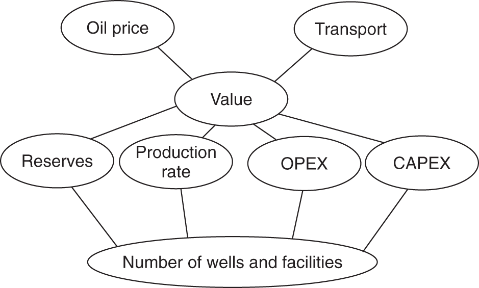
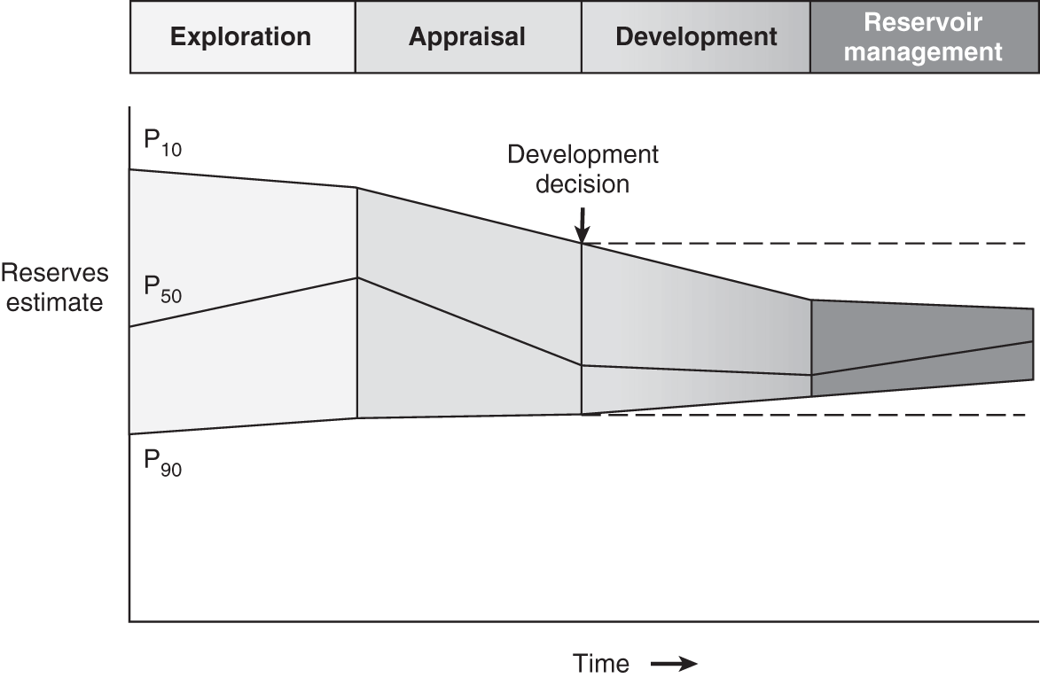
5.2 The Trap Envelope
5.2.1 Depth Conversion
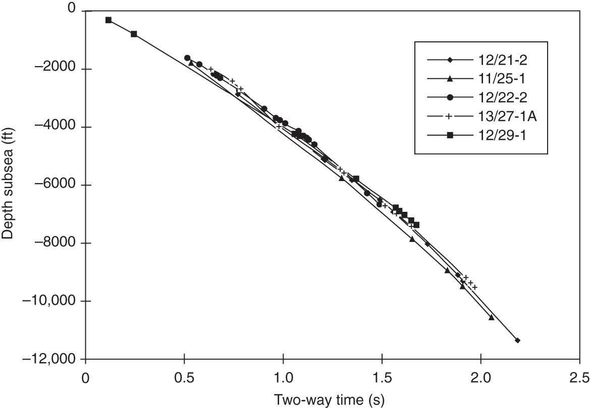
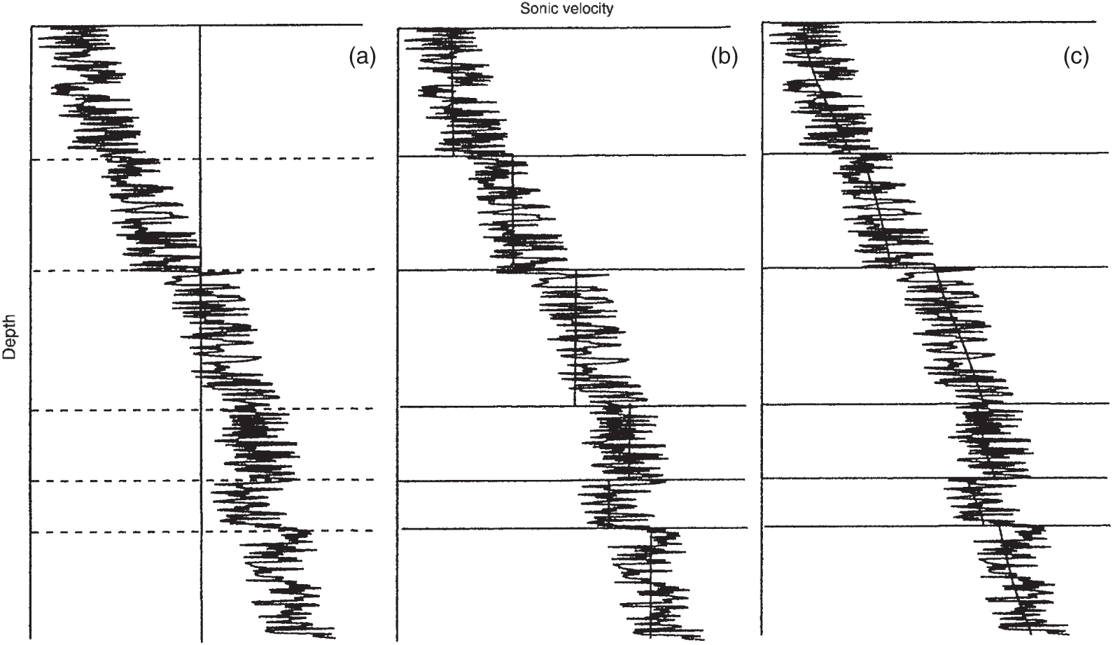
5.2.2 Mapping Surfaces and Faults
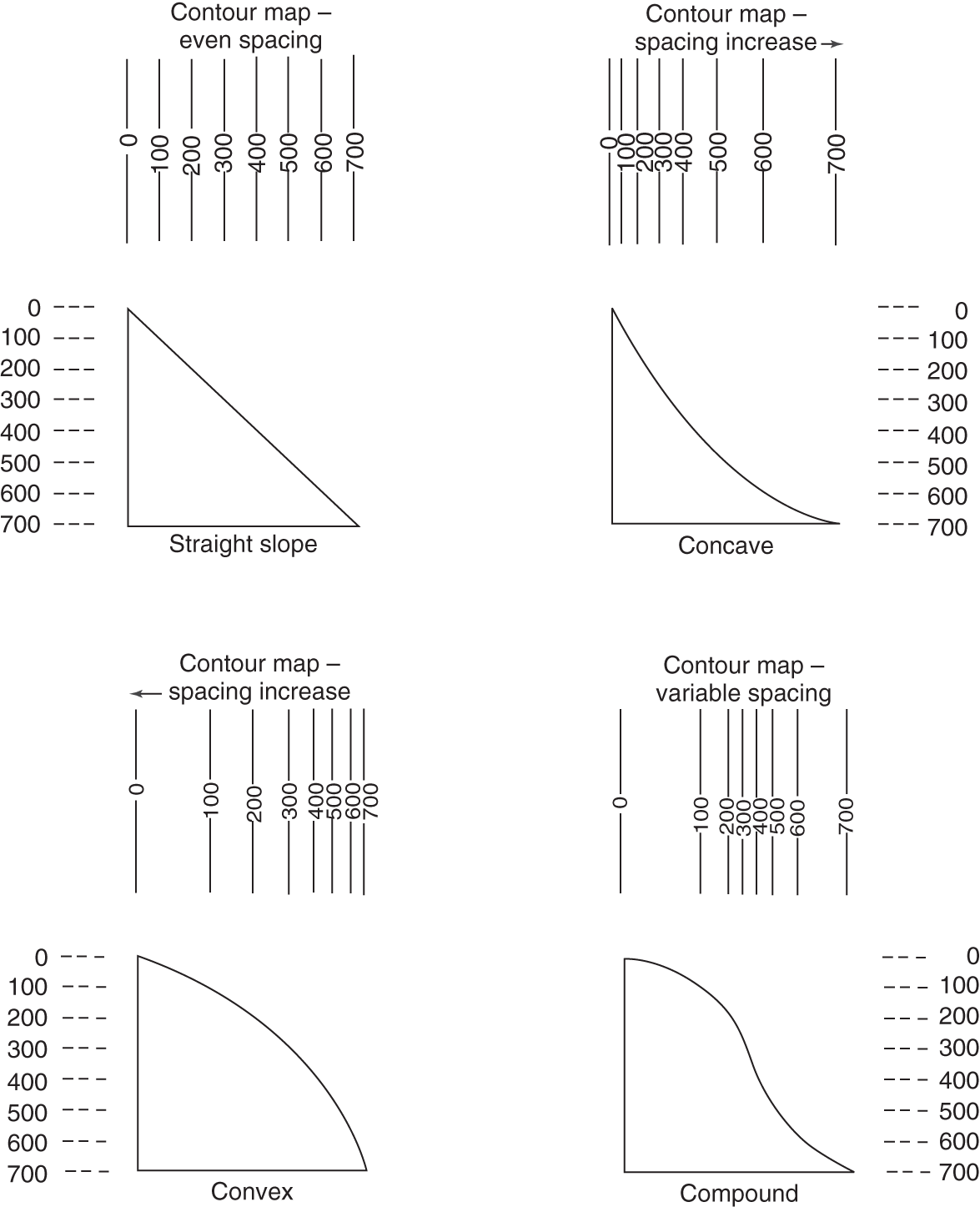
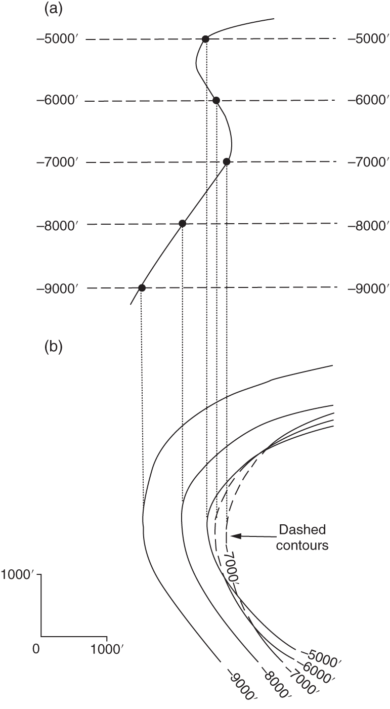
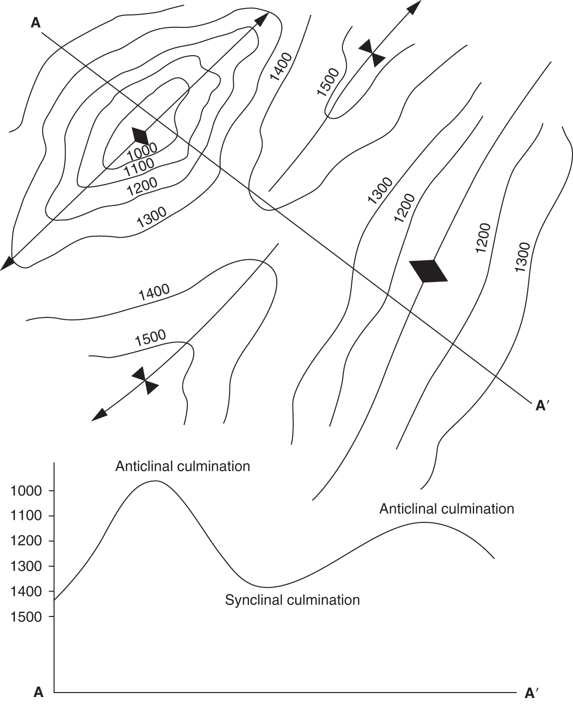
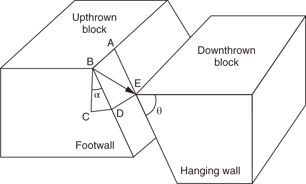
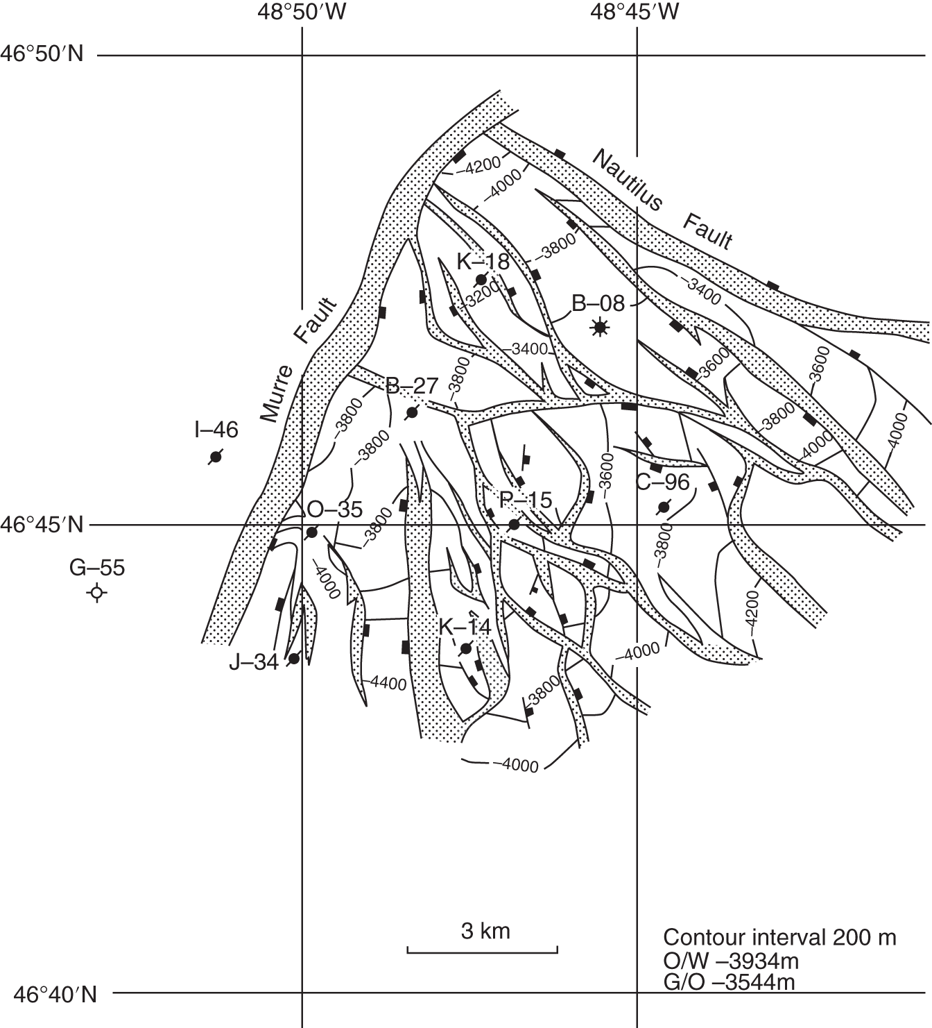
5.2.3 Spill Points
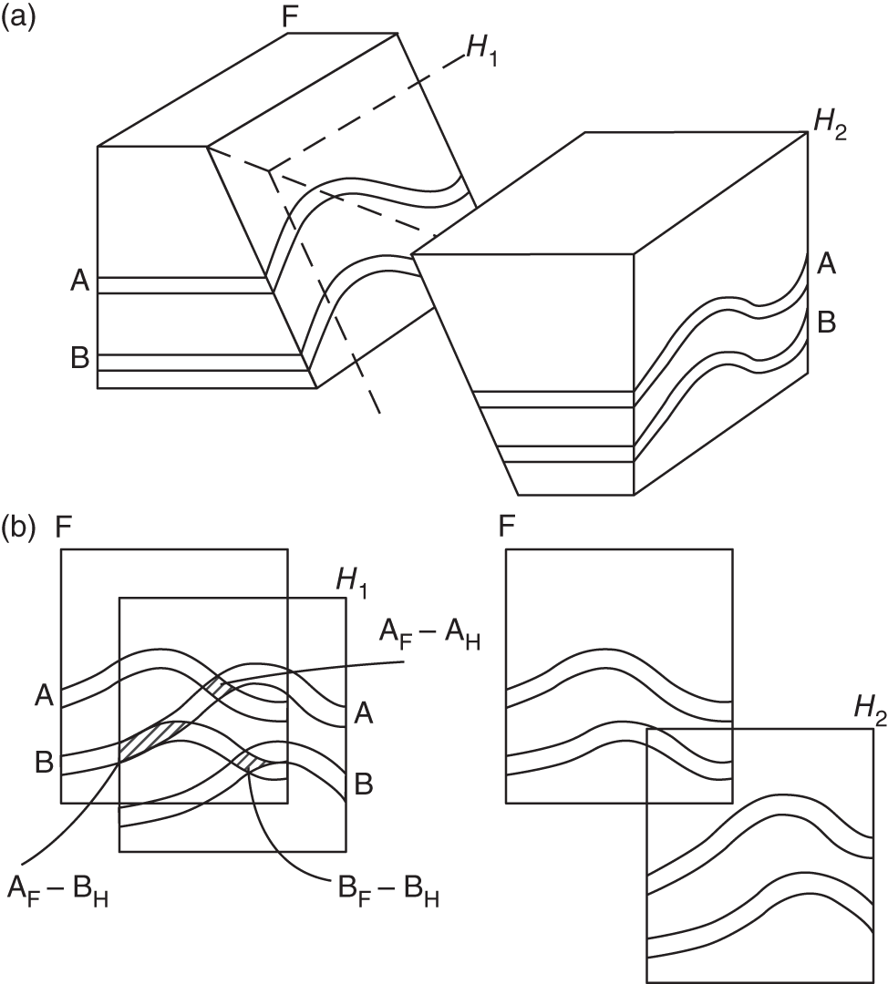
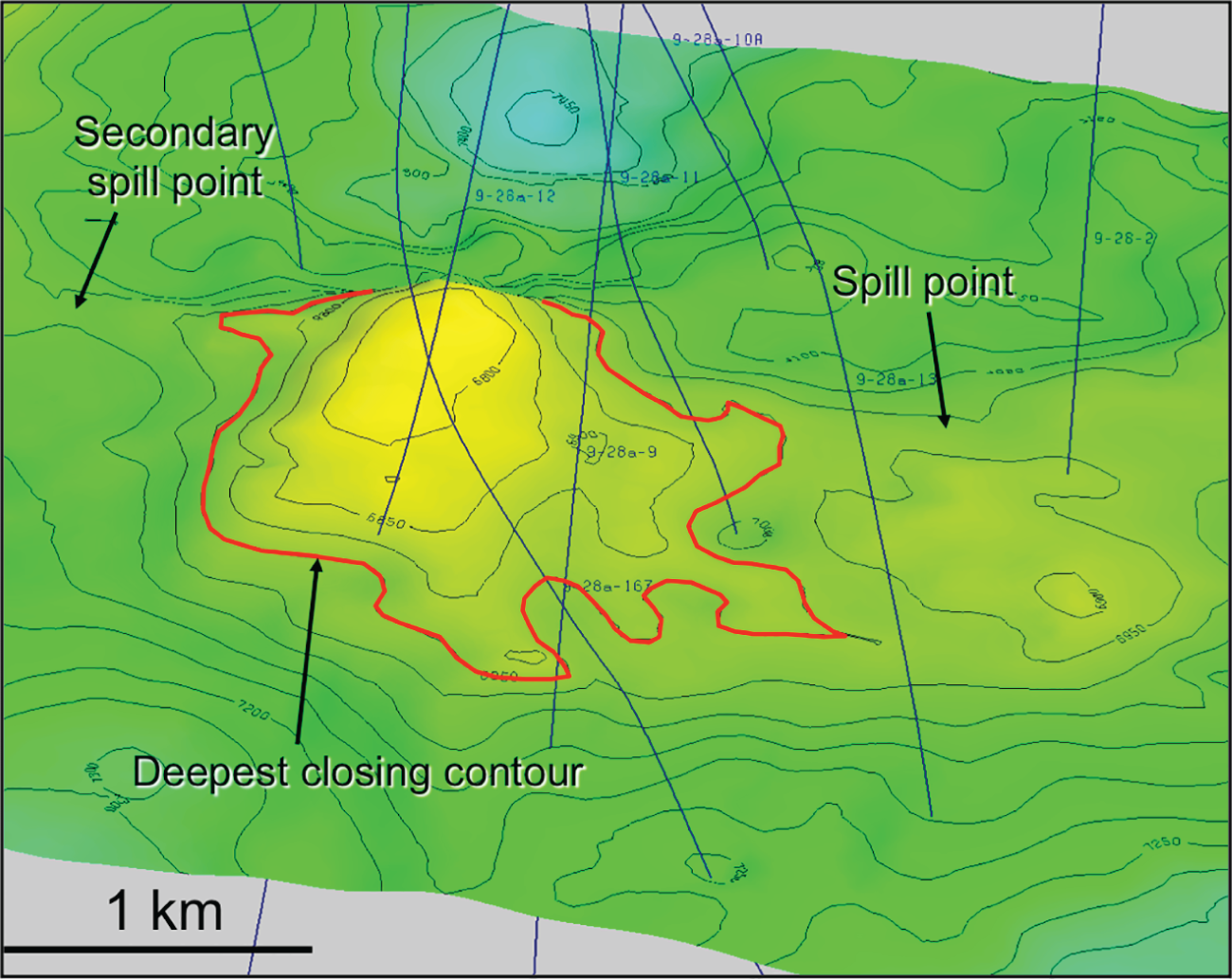
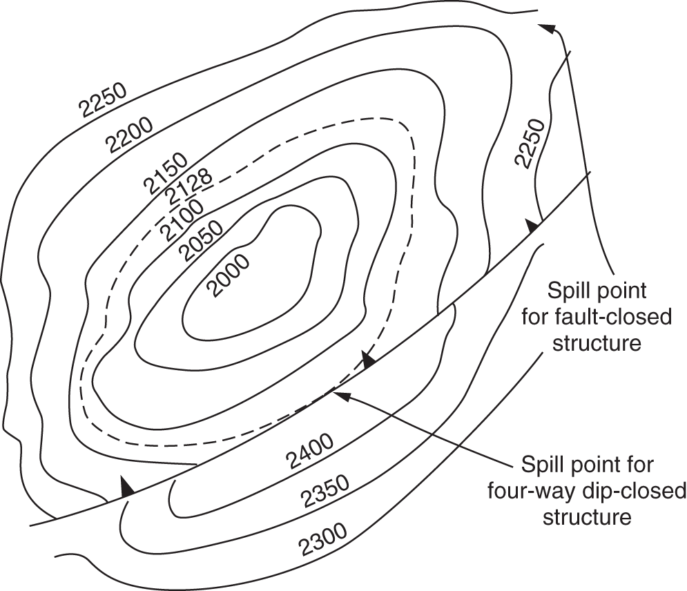
5.3 Fluid Distribution and Contacts
5.3.1 Fluid Contacts and Transition Zones
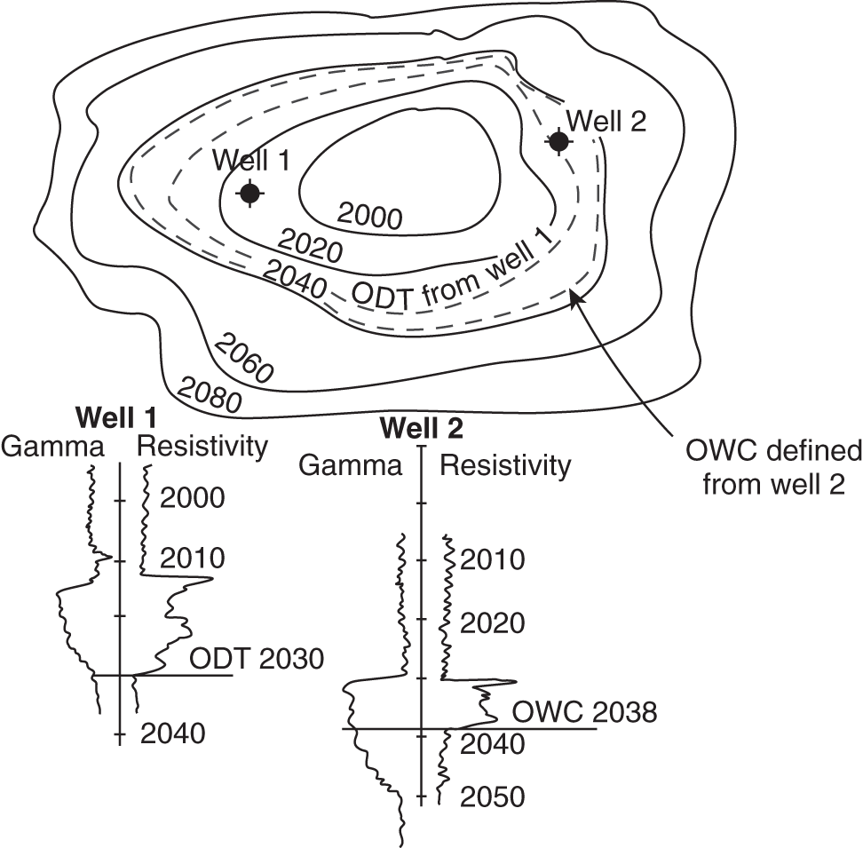
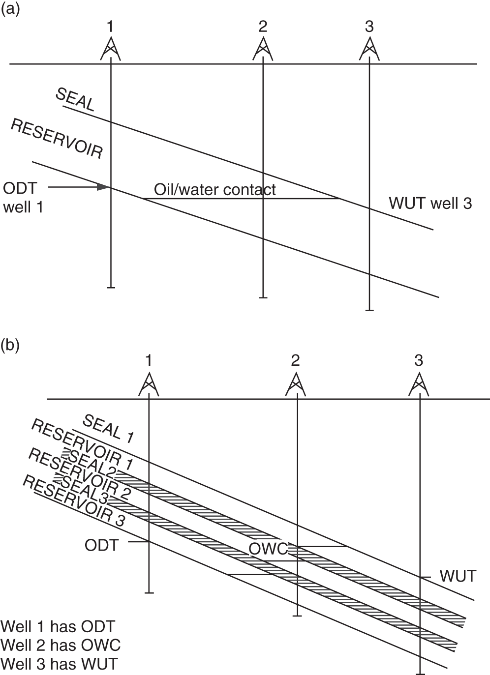
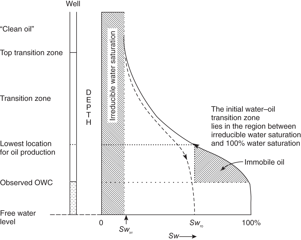
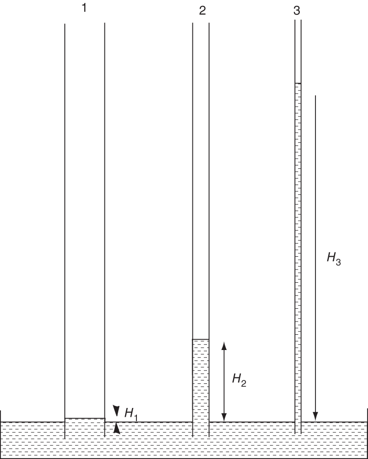
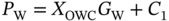
5.3.2 Intra-Field Variations in Petroleum Composition
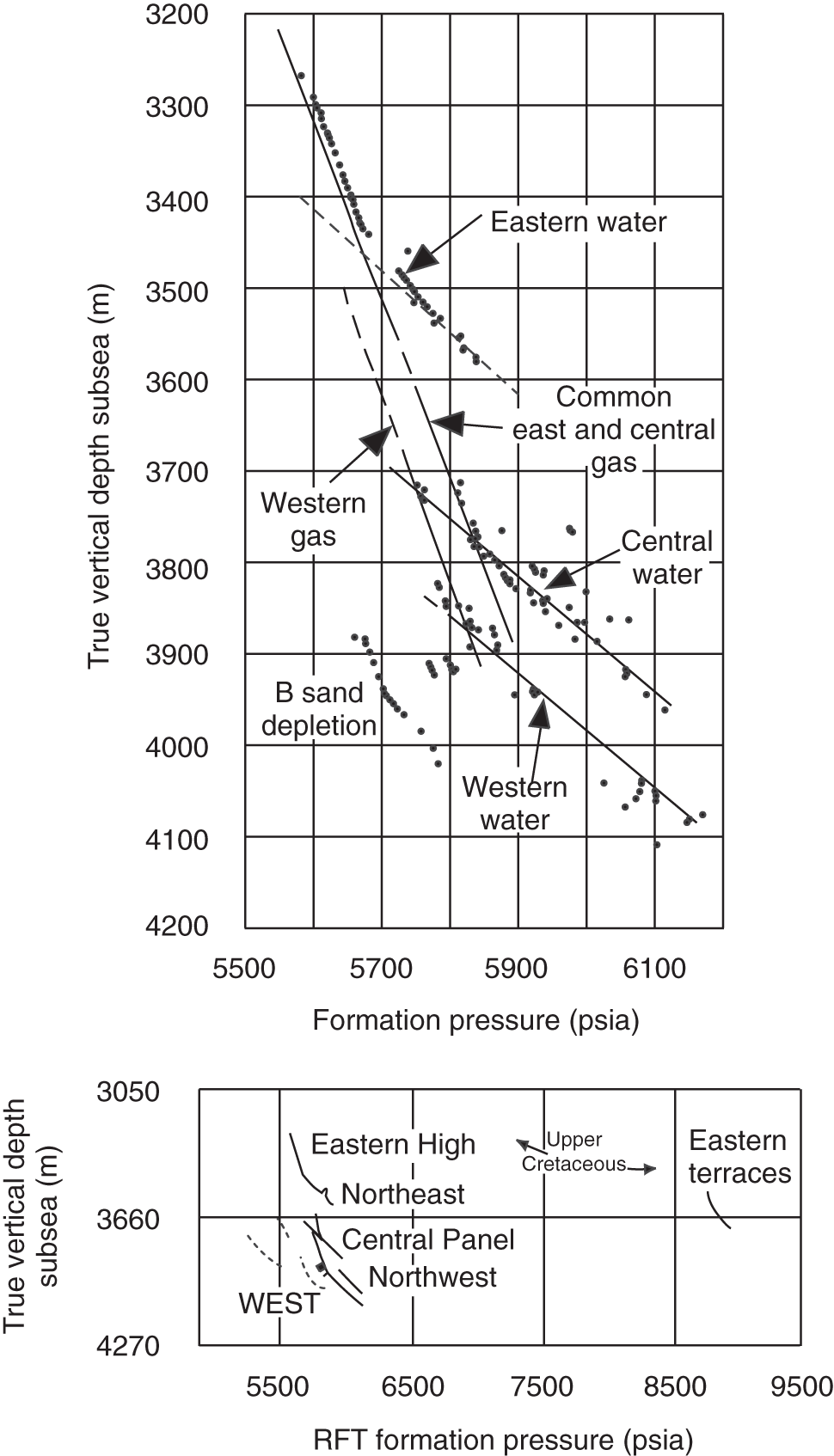
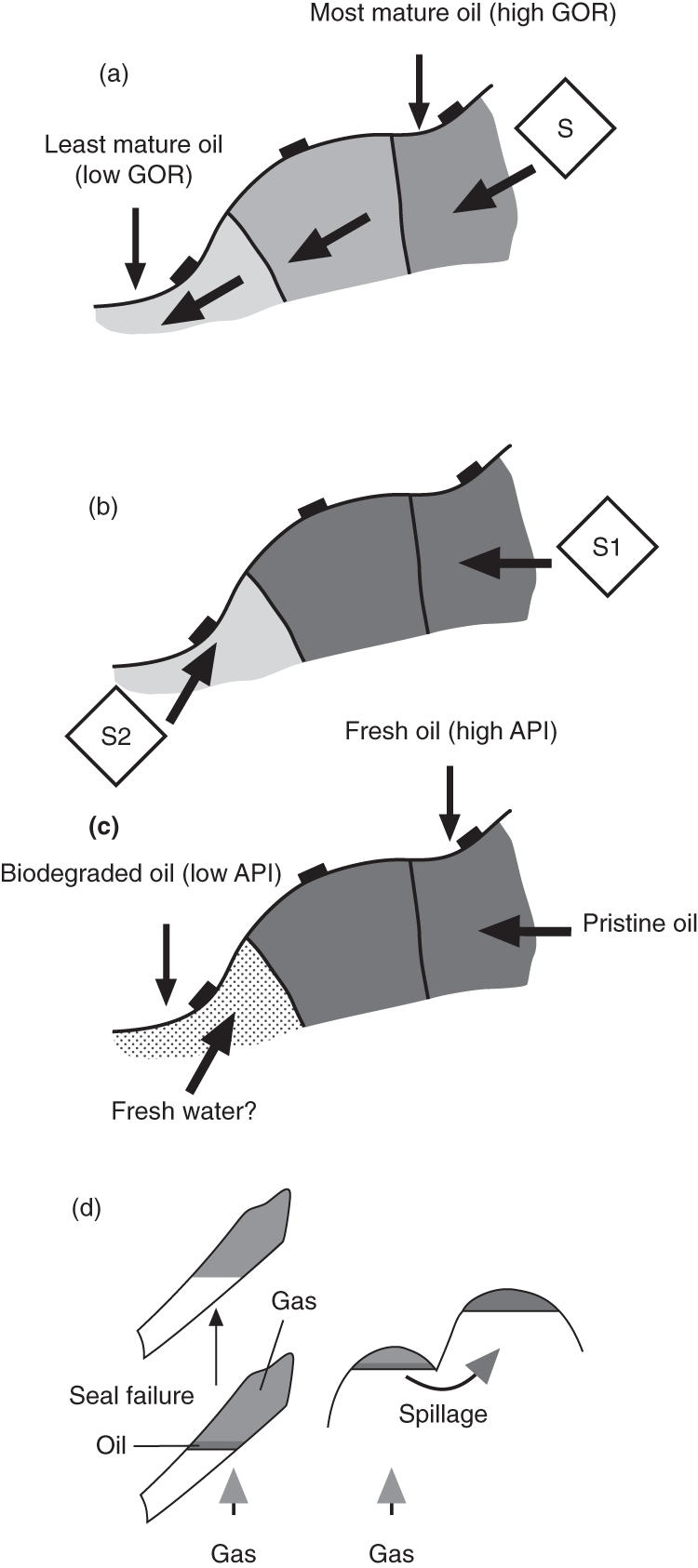
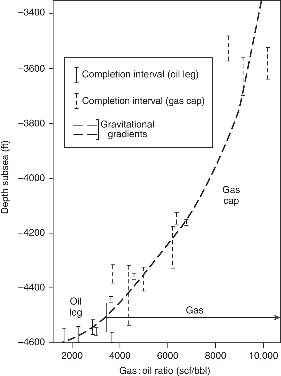
Distance (m)
Methane (Ma)
C12 (Ma)
C200 (Ma)
100
0.1
0.2
1
2000
40
80
400
5.3.3 Intra-Field Variations in Water Composition
5.4 Field Segmentation
5.4.1 Introduction
5.4.2 Barriers to Lateral Flow
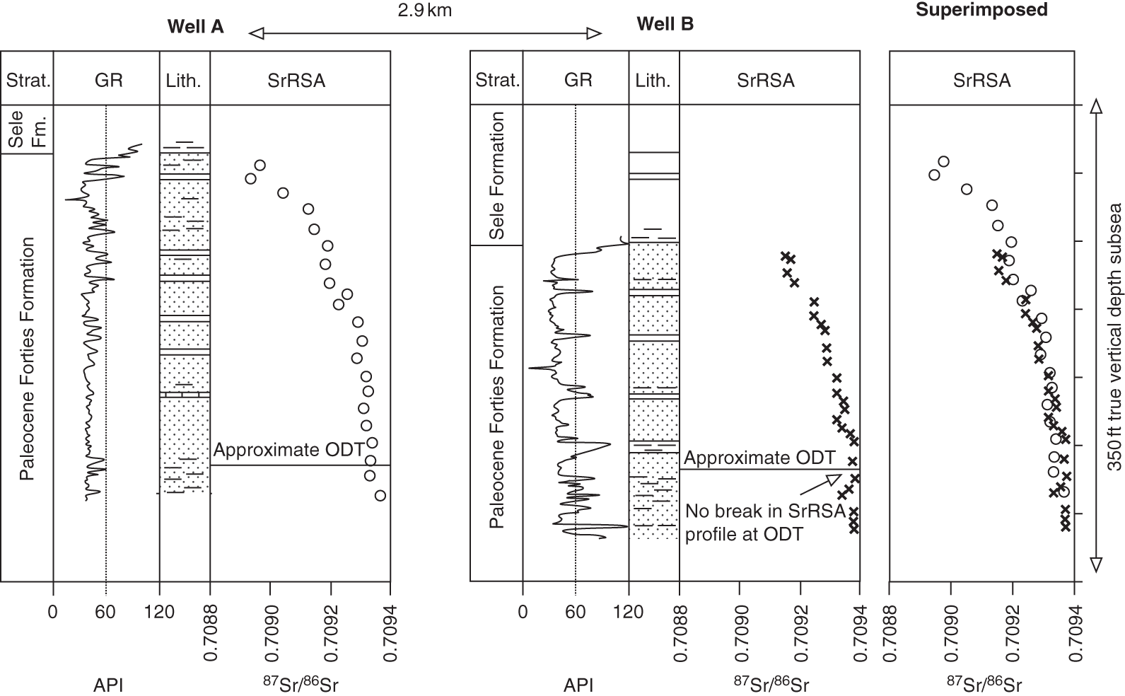
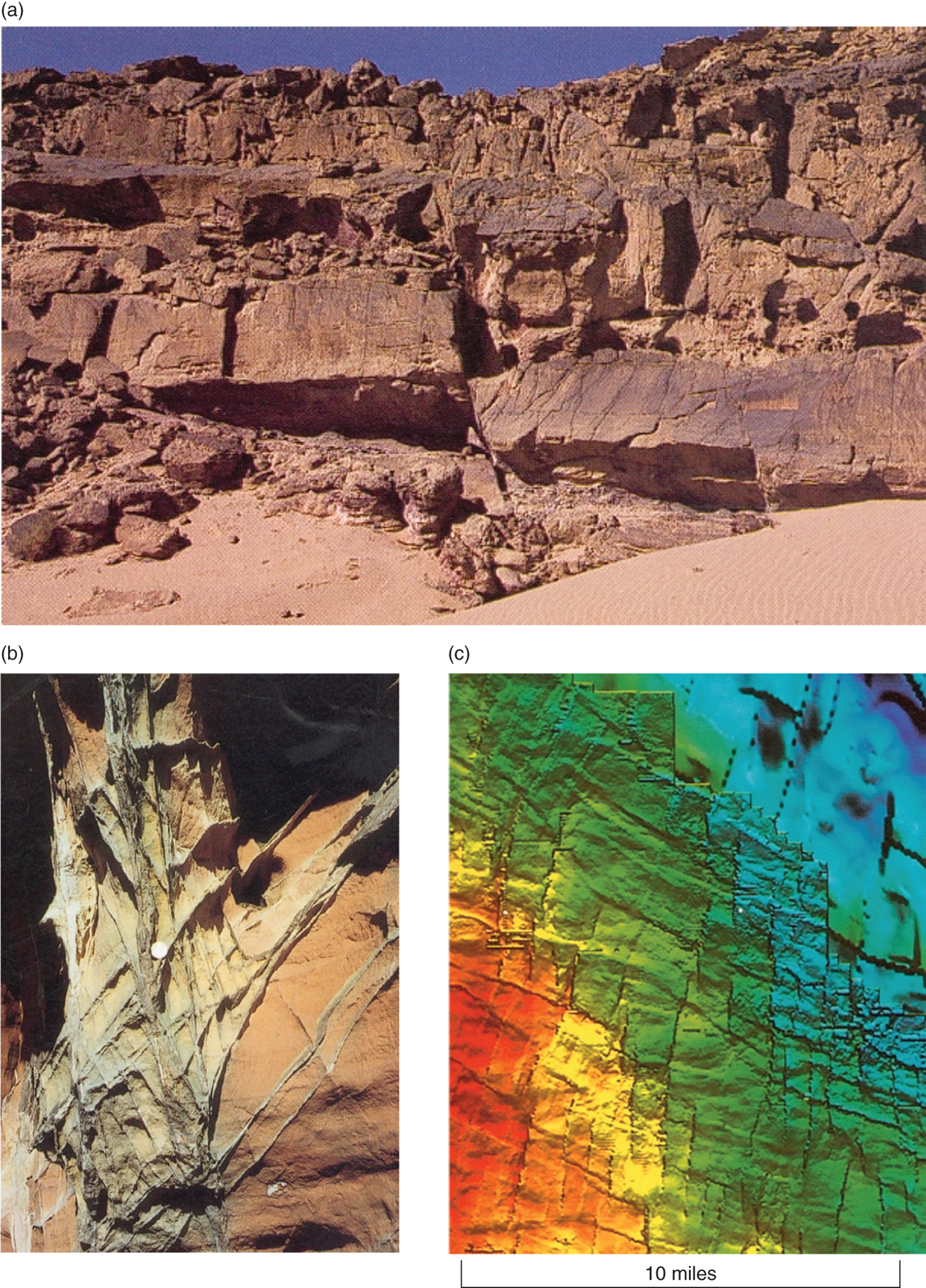
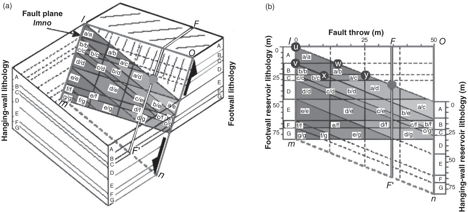
5.4.3 Barriers to Vertical Flow
5.4.4 Identification of Flow Barriers
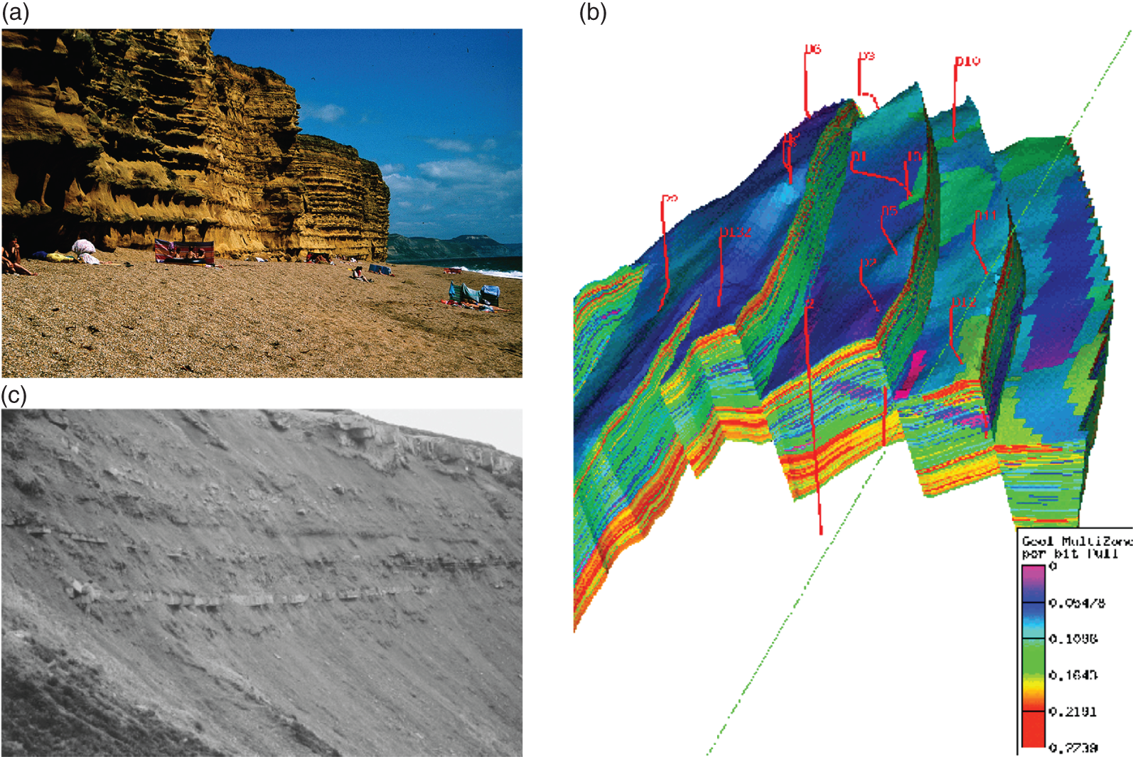
5.5 Reservoir Property Distribution
5.5.1 Introduction
5.5.2 Lithofacies and Lithotypes
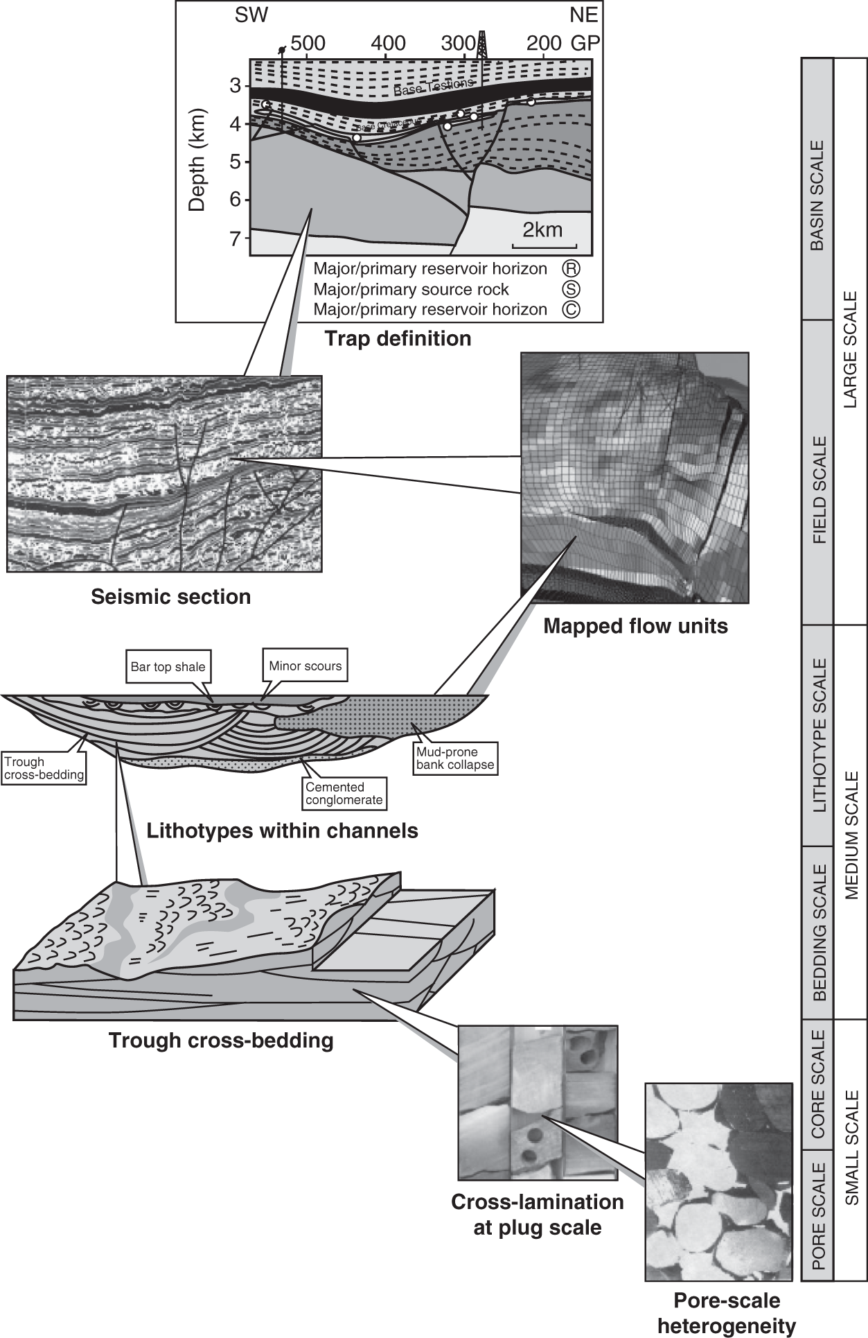
5.5.3 Reservoir Body Geometry
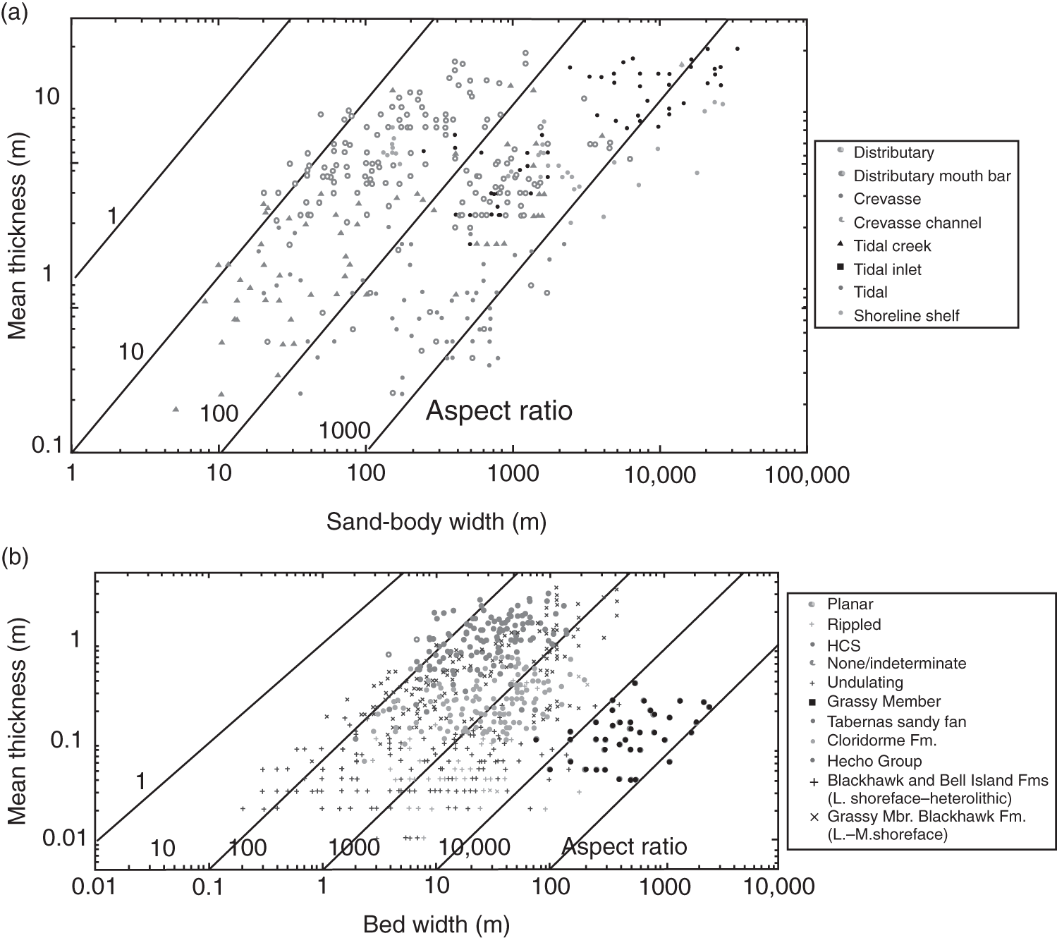
Depositional system
Element (sand body, bed, or shale)
Aspect ratio (width to thickness)
Fluvial
Low-sinuosity or meandering channel fill at <10 m thick
3 : 1–70 : 1
Fluvial
Low-sinuosity or meandering channel fill at 5–100 m thick
70 : 1–1000 : 1
Fluvial
Braided and anastamosing
10 : 1–1000 : 1
Paralic
Channel fill (distributary, crevasse)
10 : 1–100 : 1
Paralic
Depositional lobes
100 : 1–1000 : 1
Paralic
Shoreline sand bodies
200 : 1–5000 : 1 (length to width, 10 : 1–50 : 1)
Shallow-marine
Middle shoreface, beds 0.05–2 m thick
1 : 10–1 : 100
Shallow-marine
Middle shoreface, beds >2 m thick
1 : 50–1 : 200
Shallow-marine
Lower shoreface
Poor correlation of thin beds <30 cm thick
5.5.4 Reservoir Correlation
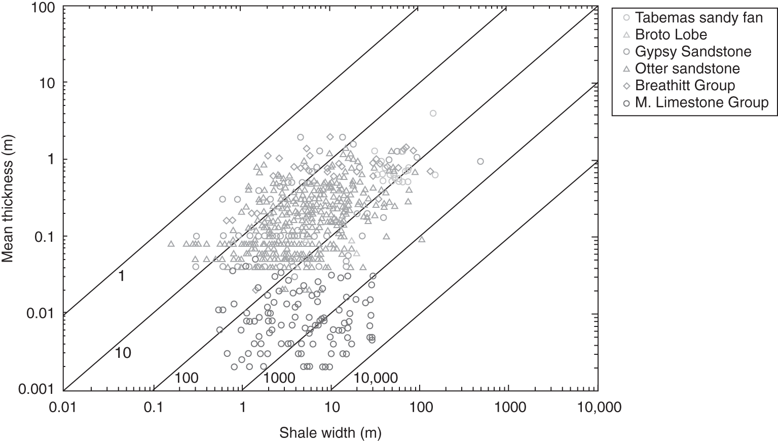
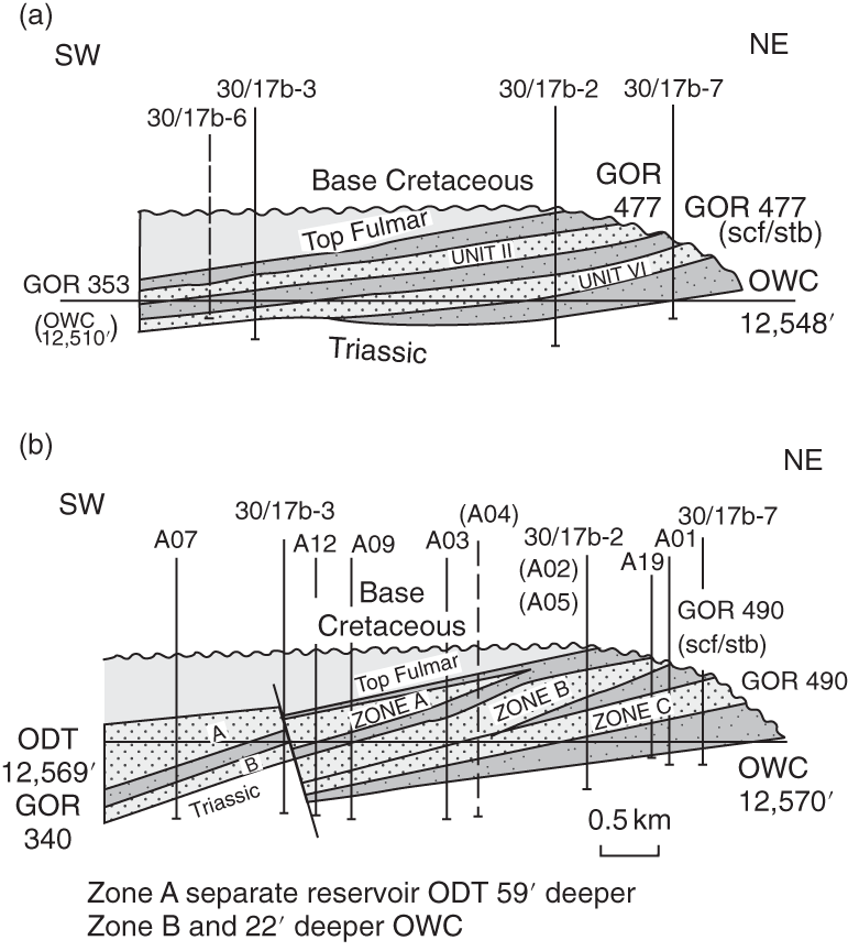
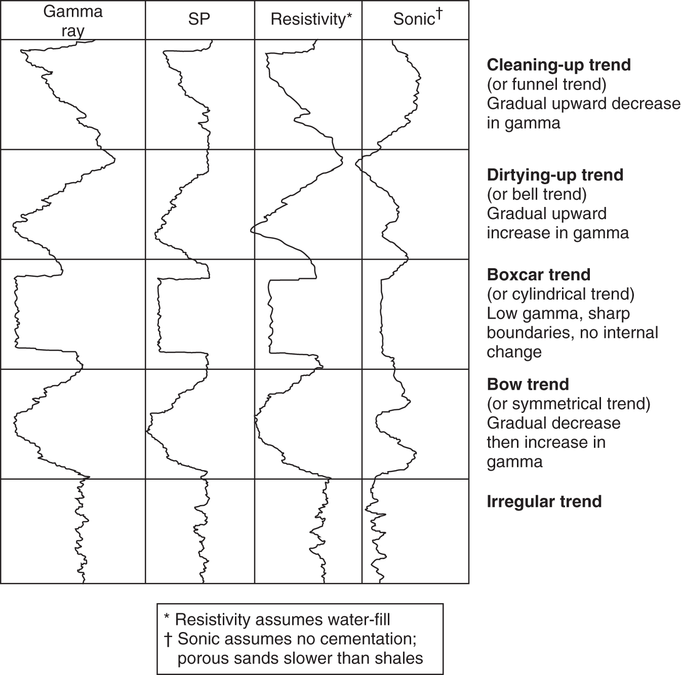
5.6 Reservoir Quality
5.6.1 Introduction
5.6.2 More Intrinsic Reservoir Properties
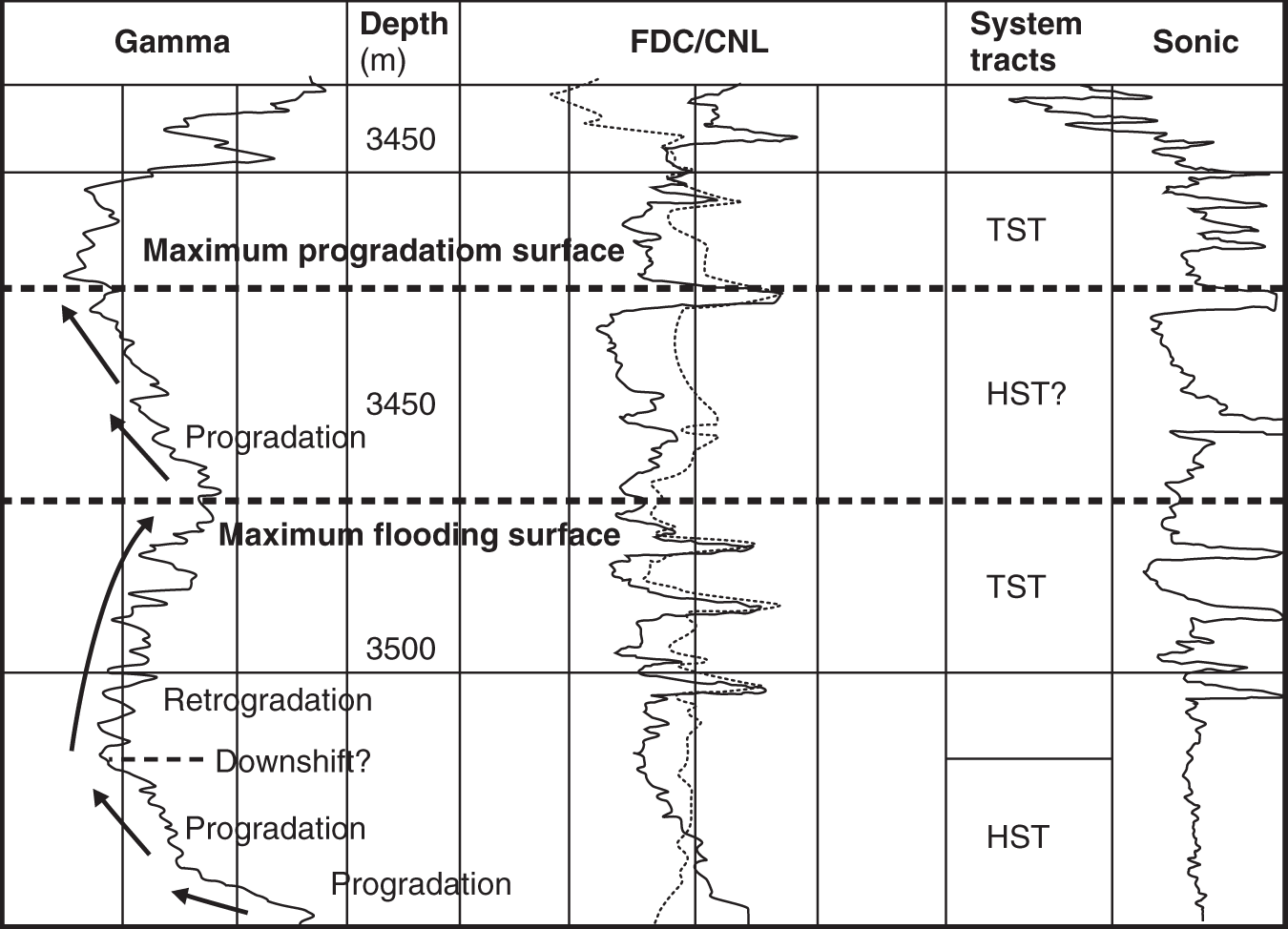
5.6.2.1 Relative Permeability
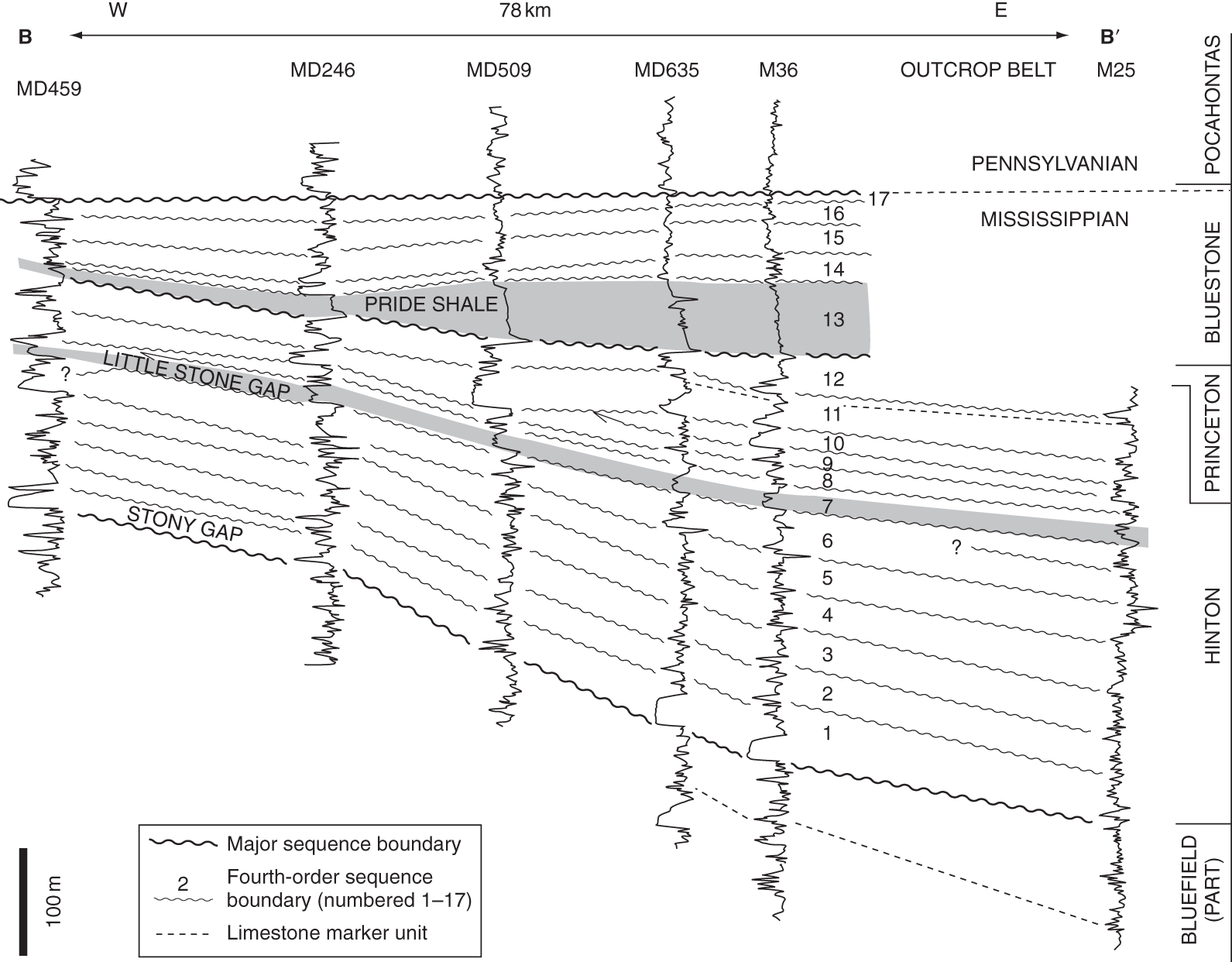
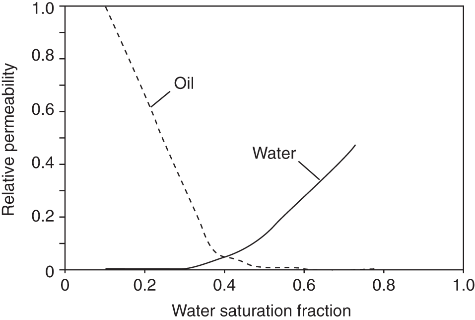
5.6.2.2 Wettability
5.6.2.3 Resistivity, Cementation, and Tortuosity Factors

5.6.3 Controls on Reservoir Quality
5.6.4 Compaction and Cementation in Sandstones
5.6.4.1 Sand Compaction
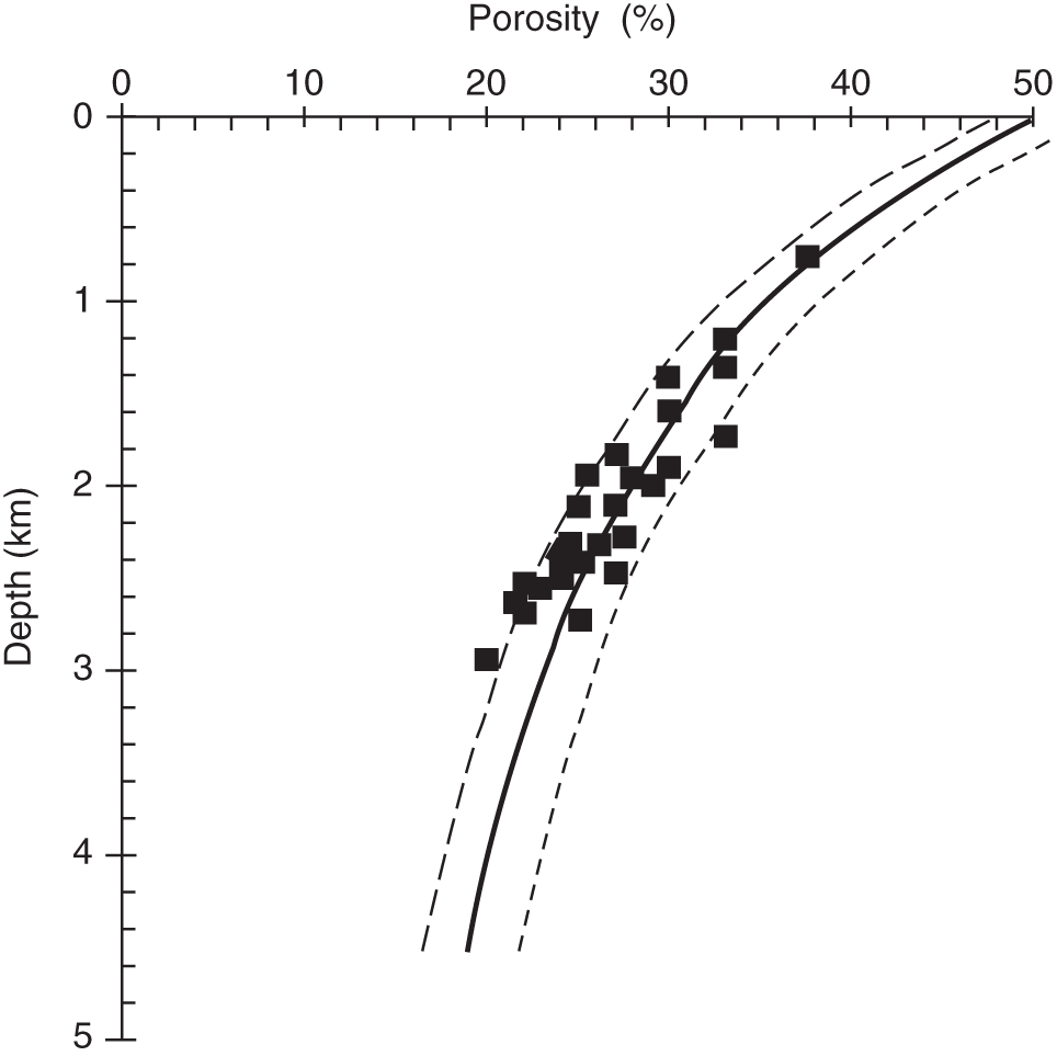
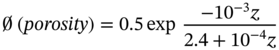
5.6.4.2 Sand Cementation
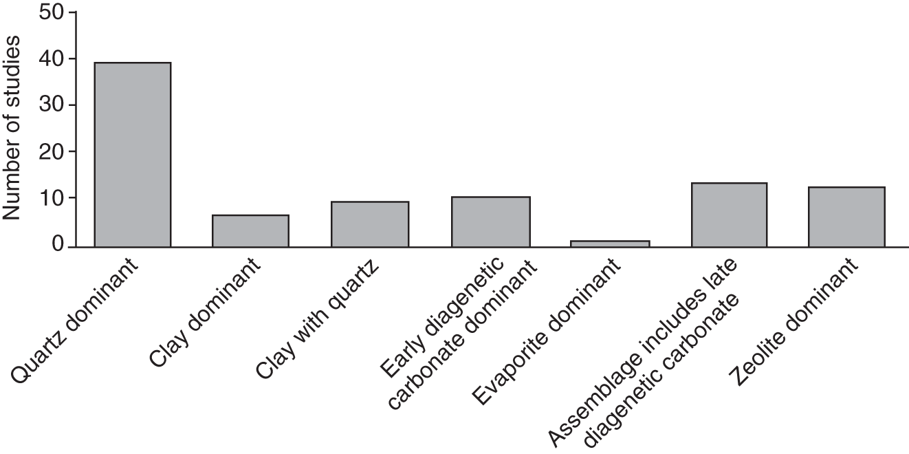
5.6.5 Compaction and Cementation in Limestones
5.6.5.1 Near-Surface Processes
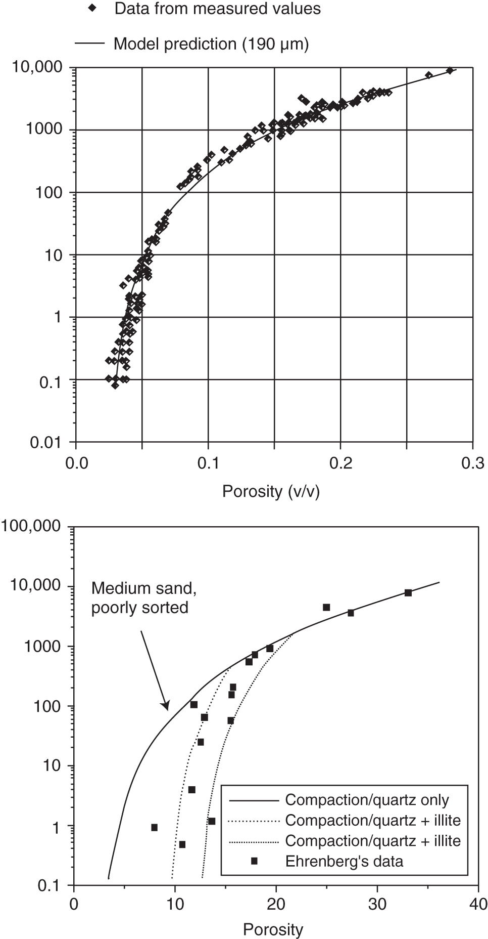
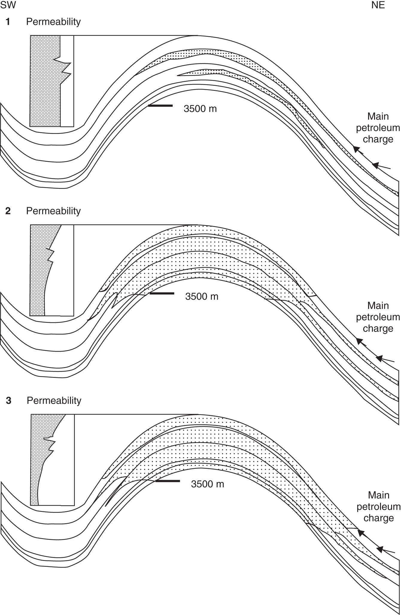
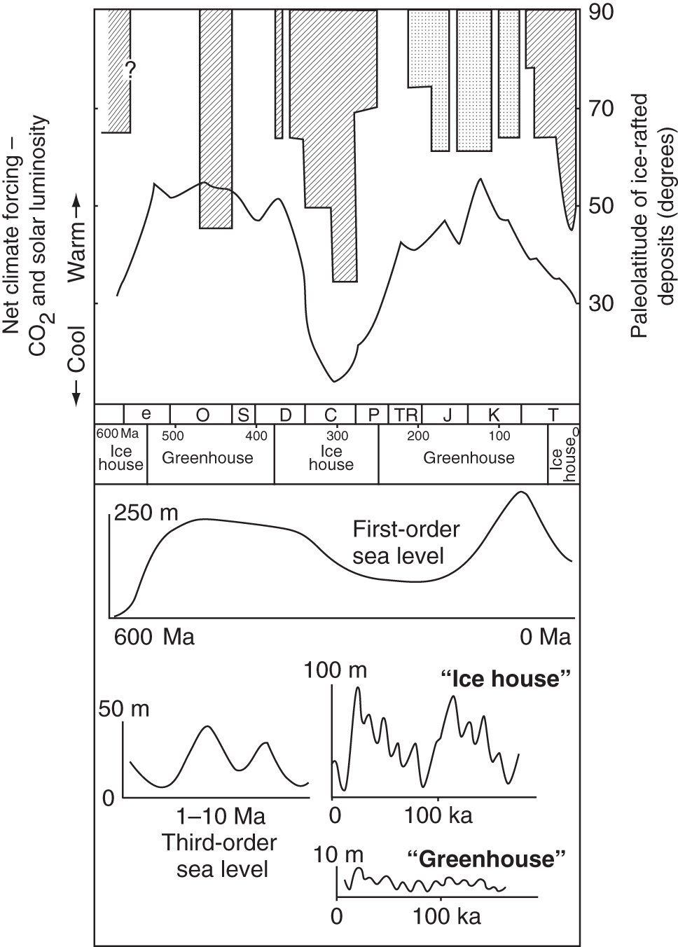
Sea-level change
Climate type
Amplitude
Frequency
“Temperature”
Rainfall
1
Low
High
Greenhouse
Humid
2
Low
High
Greenhouse
Arid
3
Moderate
High
Ice house
Humid
4
Moderate
High
Ice house
Arid
5
Large
High
Ice house
Humid
6
Large
High
Ice house
Arid
7
Large
Low
Greenhouse/ice house
Humid
8
Large
Low
Greenhouse/ice house
Arid
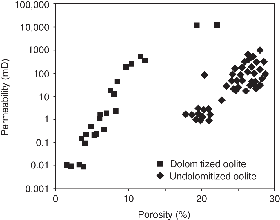
5.6.5.2 Compaction and Burial Processes
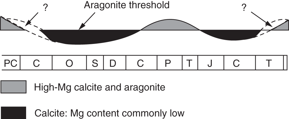
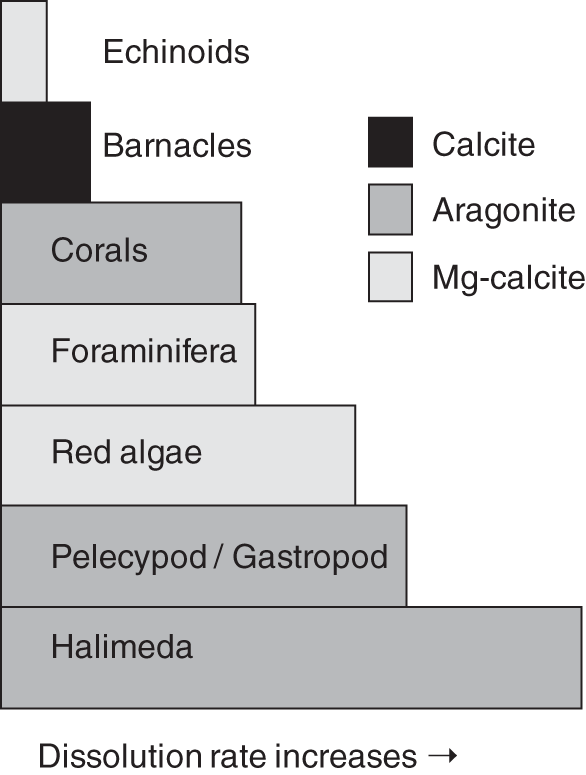
5.7 Reservoir Description from Seismic Data
5.7.1 Introduction
5.7.2 Lithology Description
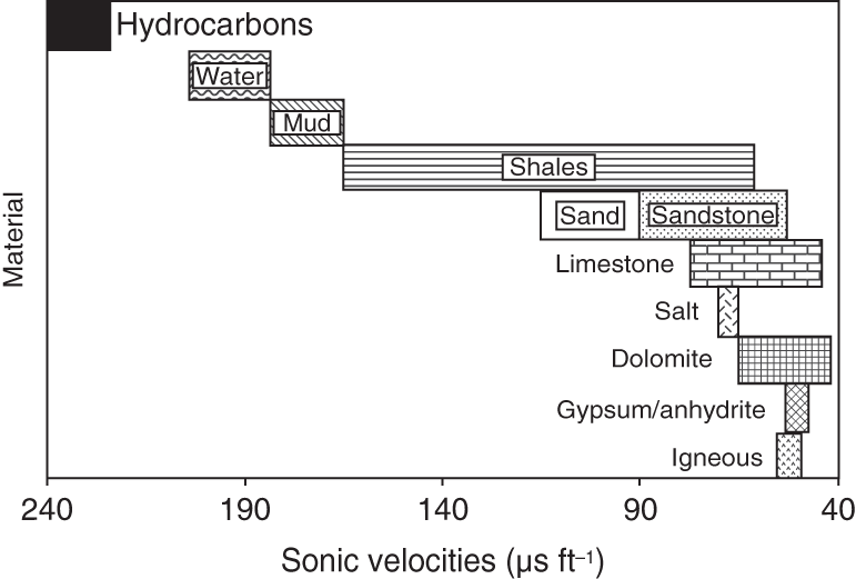
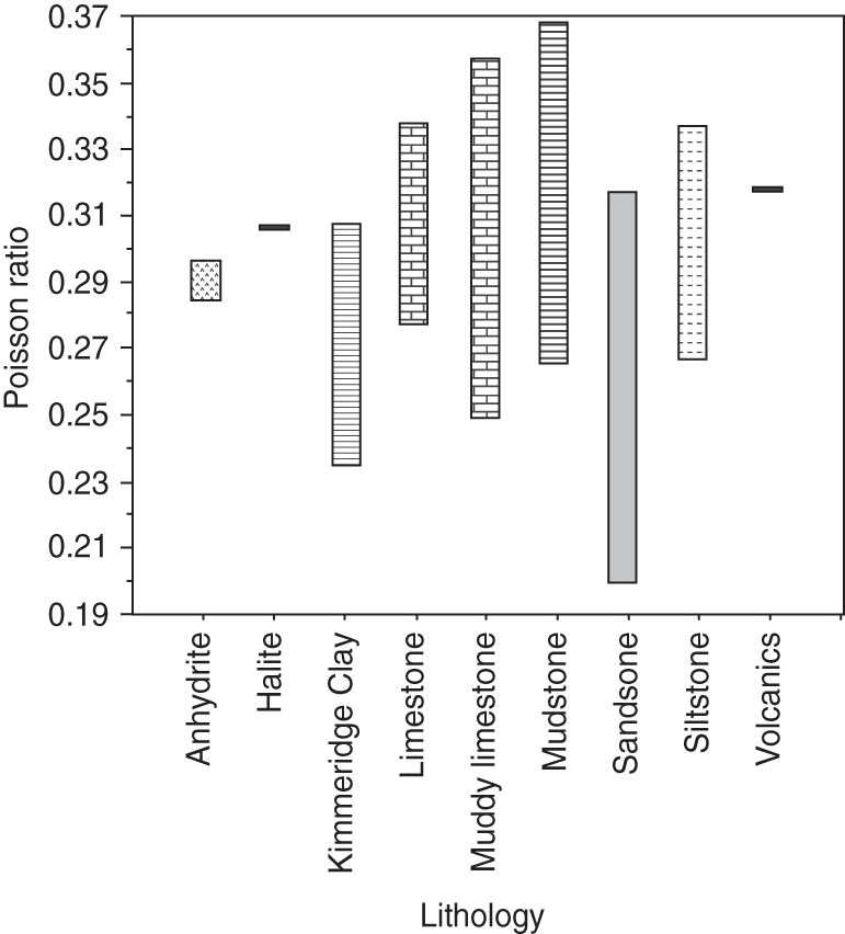
5.7.3 Porosity Determination

5.7.4 Lateral Variations and Reservoir Heterogeneity
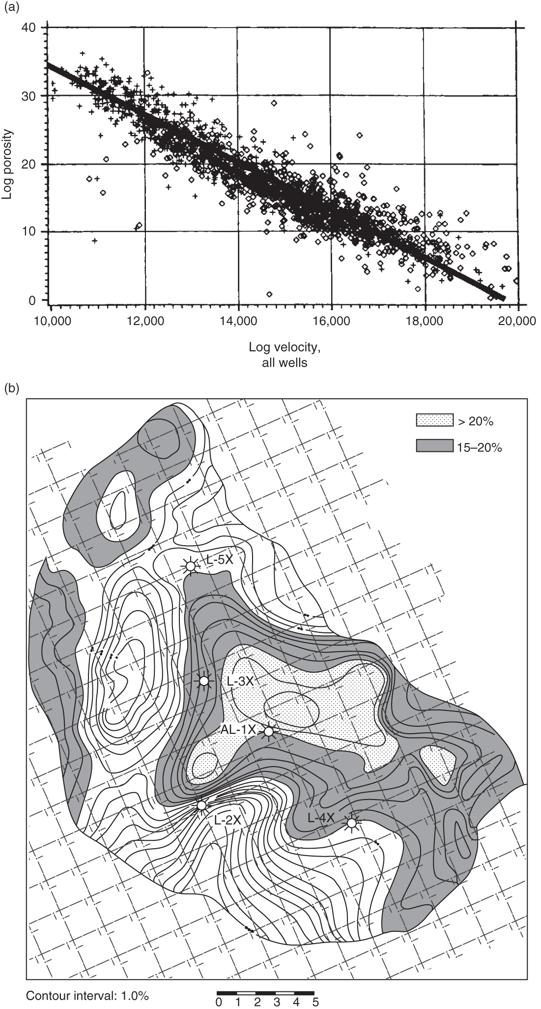
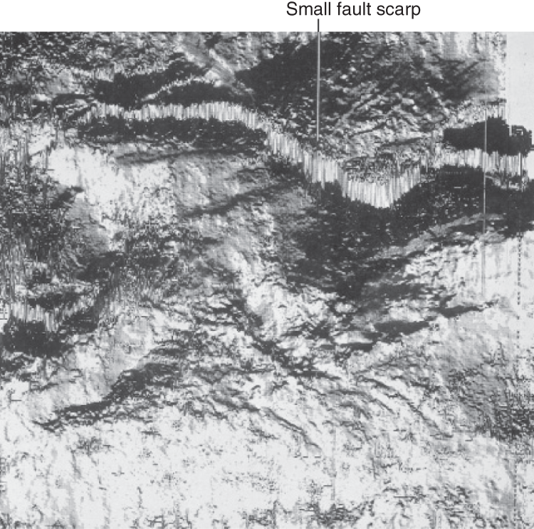
5.7.5 Reservoir Correlation
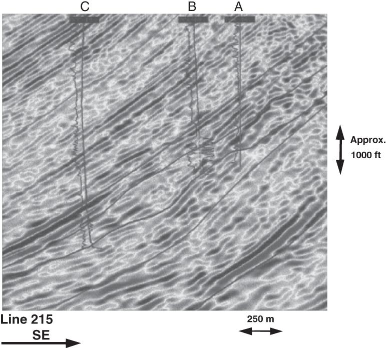
5.7.6 Identification of Fluid Type and Contacts
5.8 Petroleum in Place, Reservoir Models, and Reserves
5.8.1 Introduction
5.8.2 Petroleum in Place
5.8.3 Geologic Models
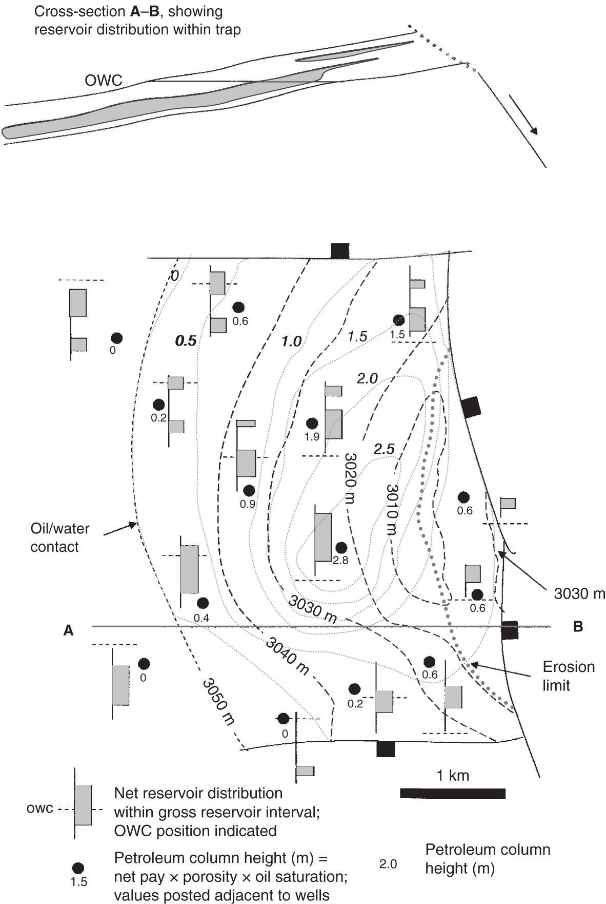
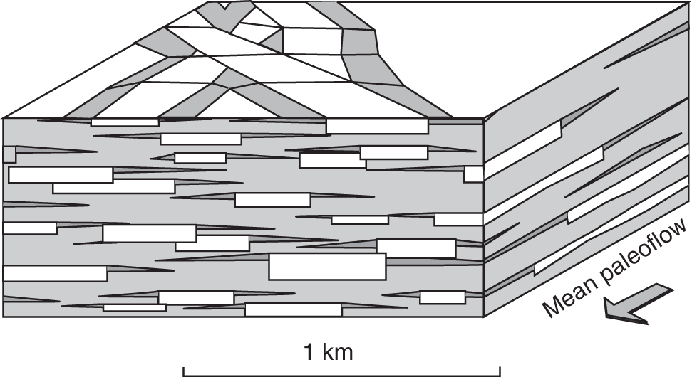
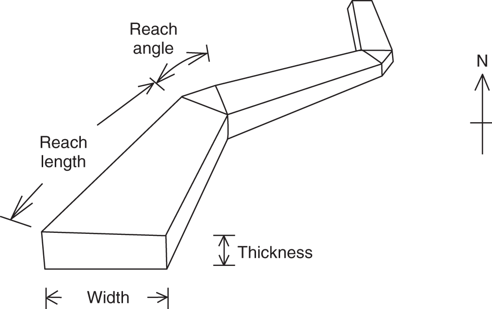

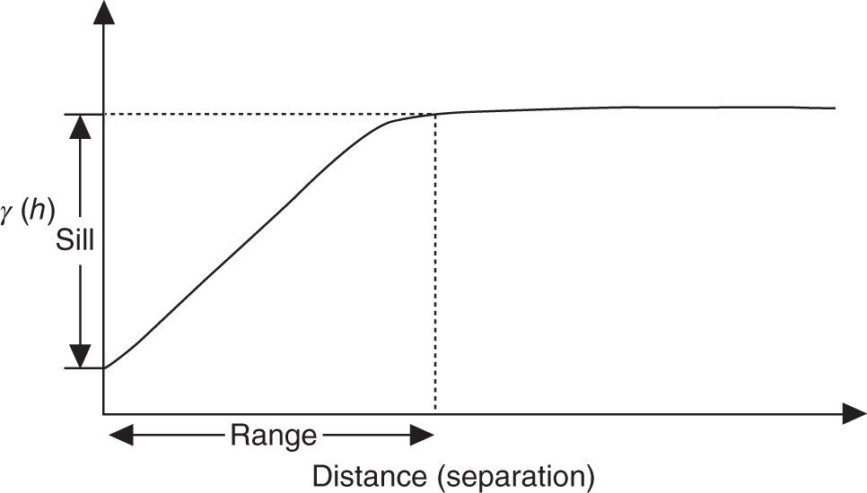
5.8.4 Reservoir Models
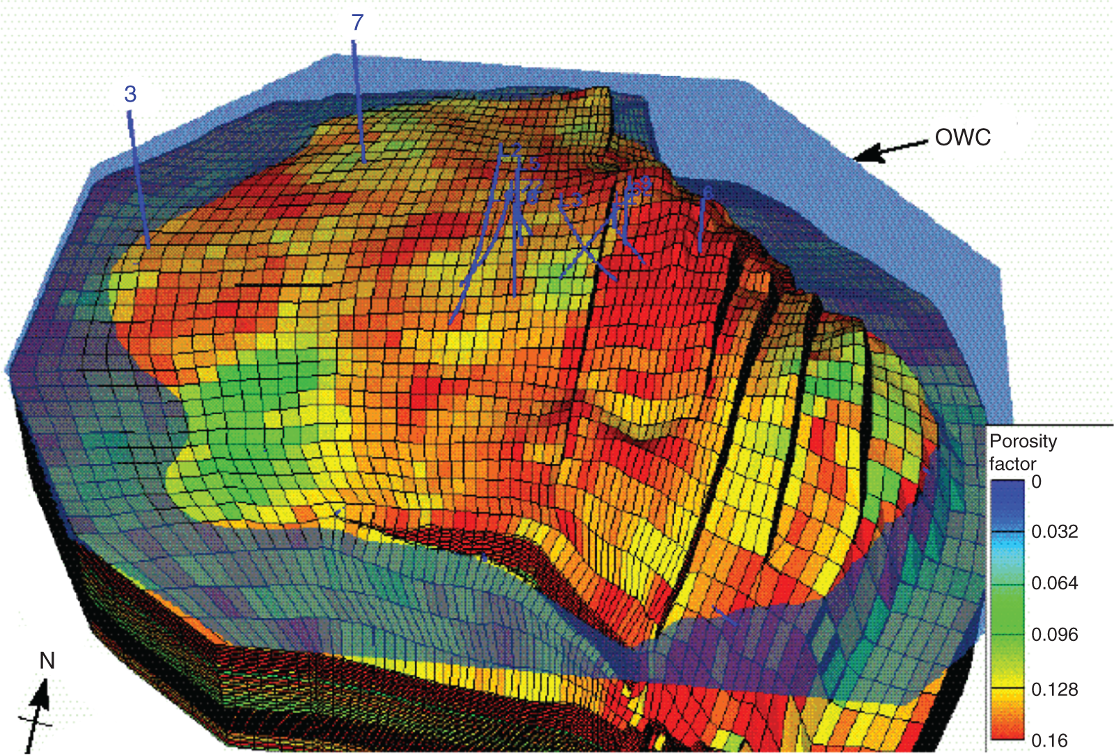
5.8.5 Reserves
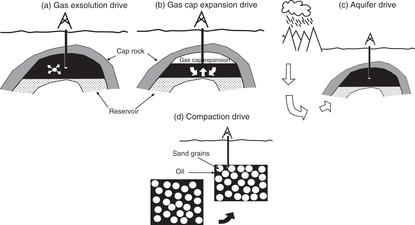
North Sea
Trinidad
Field
Recovery factor (%)
Field (Pliocene and Miocene reservoirs throughout)
Recovery factor (%)
Alwyn (Middle Jurassic Brent Group)
50
Balata
6
Alwyn (Lower Jurassic Statfjord Formation)
35
Barrackpore/Penal
11
Auk (Zechstein + Rotliegend)
19
Brighton Marine
11
Brae Central (Upper Jurassic)
40
Cat’s Hill
32
Brae South (Upper Jurassic)
33
Coora Quarry
13
Buchan (Devonian, fractured)
16
Forest Reserve
16
Claymore (Lower Cretaceous)
45
Fyzabad
22
Cormorant (Middle Jurassic Brent Group)
39
Guaya Guayare
19
Ekofisk (Upper Cretaceous)
40
North Soldado
16
Forties (Paleocene)
57
Oropuche
9
Fulmar (Upper Jurassic)
57
Palo Seco
12
Glamis (Upper Jurassic)
50
Parrylands
10
Maureen (Paleocene)
54
Rock Dome
17
Piper (Upper Jurassic)
70
Tabaquite
22
Case Histories
5.9 Kadanwari Field, Pakistan
5.9.1 Introduction
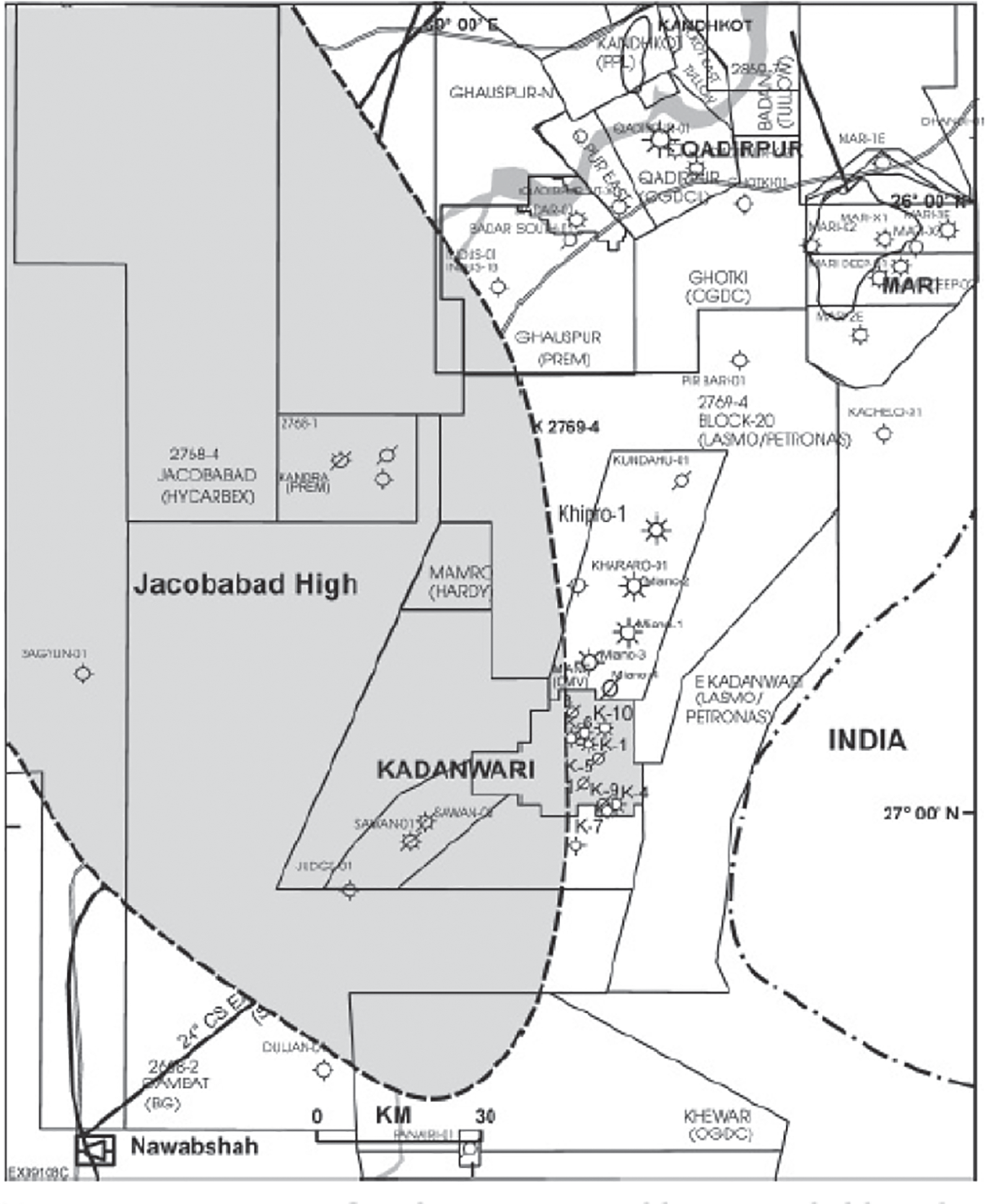
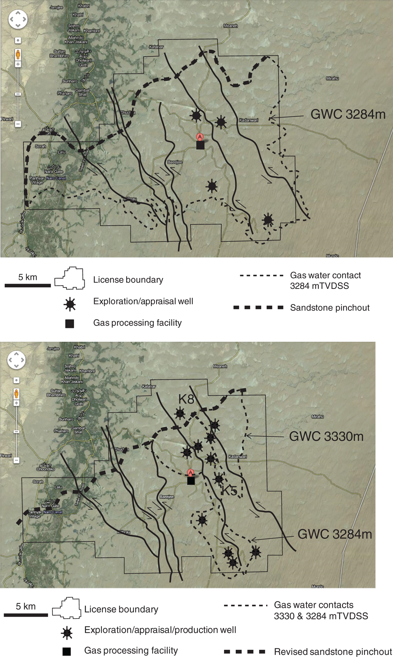
5.9.2 Re-Evaluation of Seismic Data over Kadanwari
5.10 Pedernales Field, Venezuela
5.10.1 Introduction
5.10.2 Geology of the Area
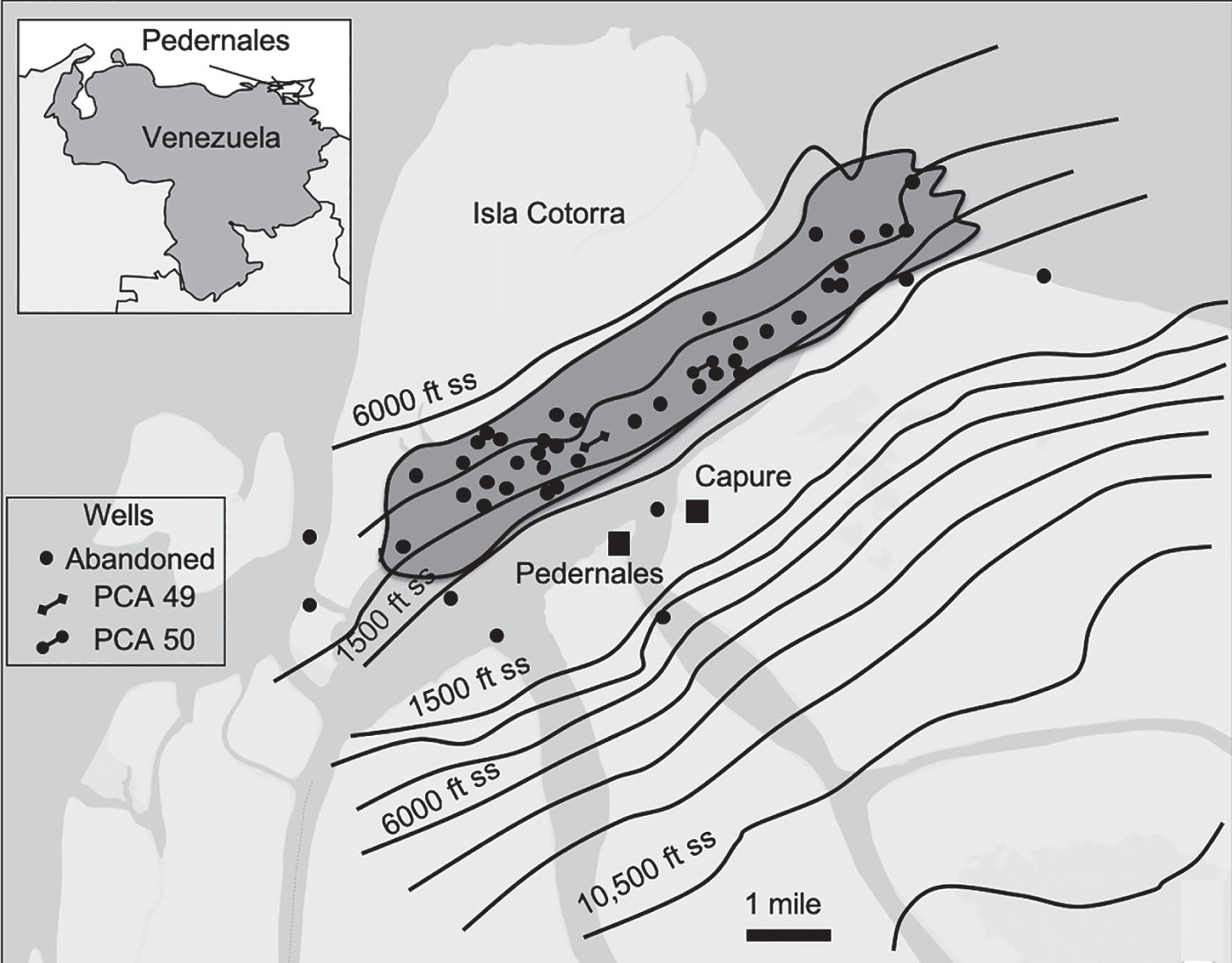
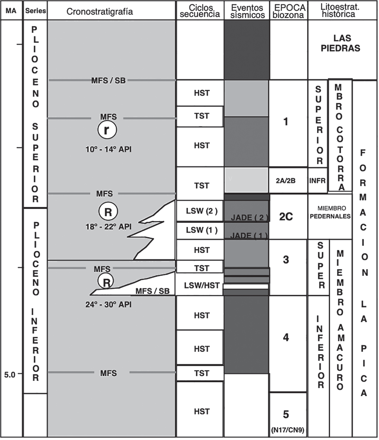
5.10.3 History of Exploration and Production
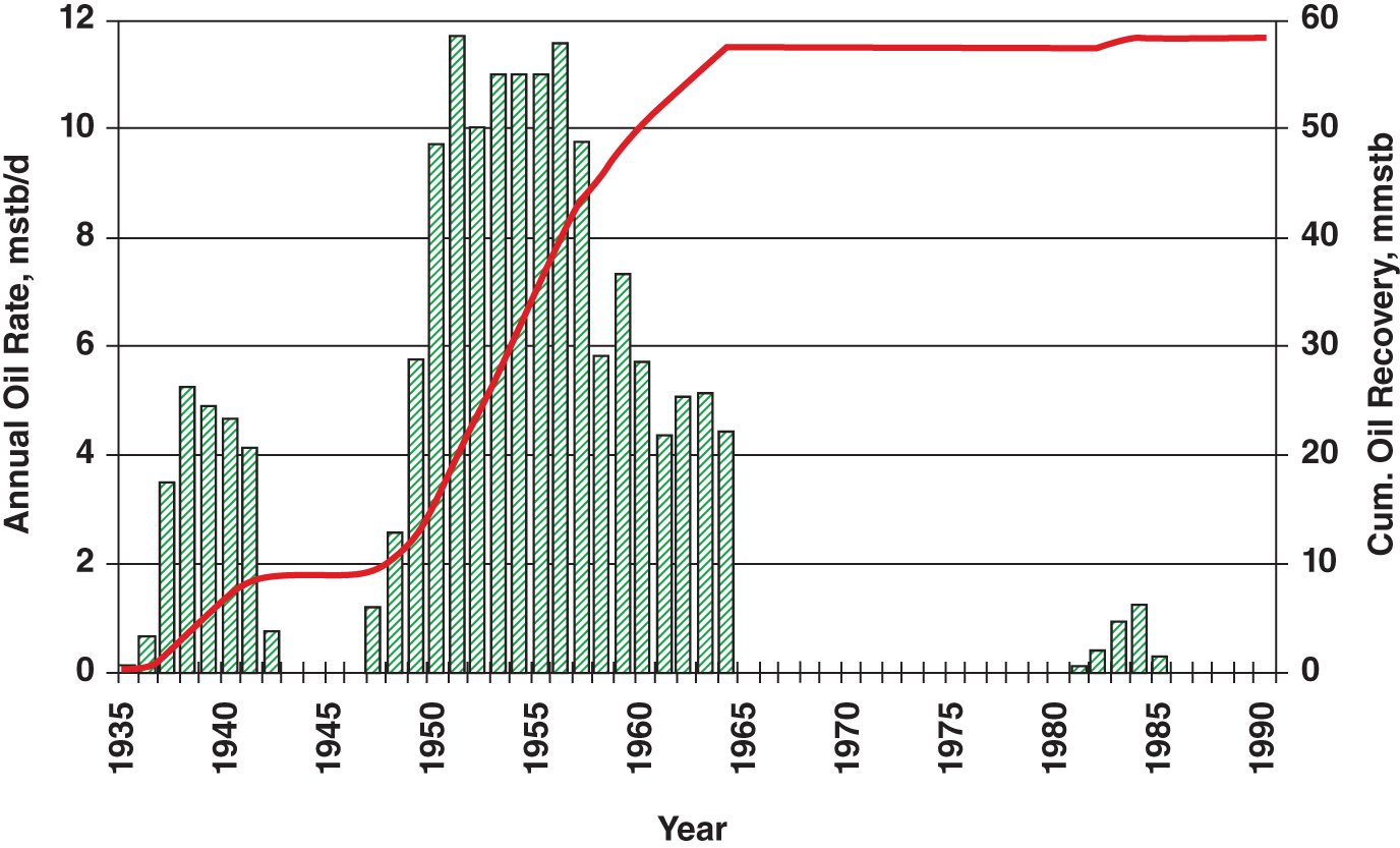
5.10.4 Field Reactivation, 1990s
Reservoir interval
STOOIP p90
STOOIP p50
STOOIP p10
Cotorra
985
1353
1842
Pedernales
3892
4611
5488
Amacuro
457
587
749
Miocene
415
572
762
5749
7123
8841
Further Reading