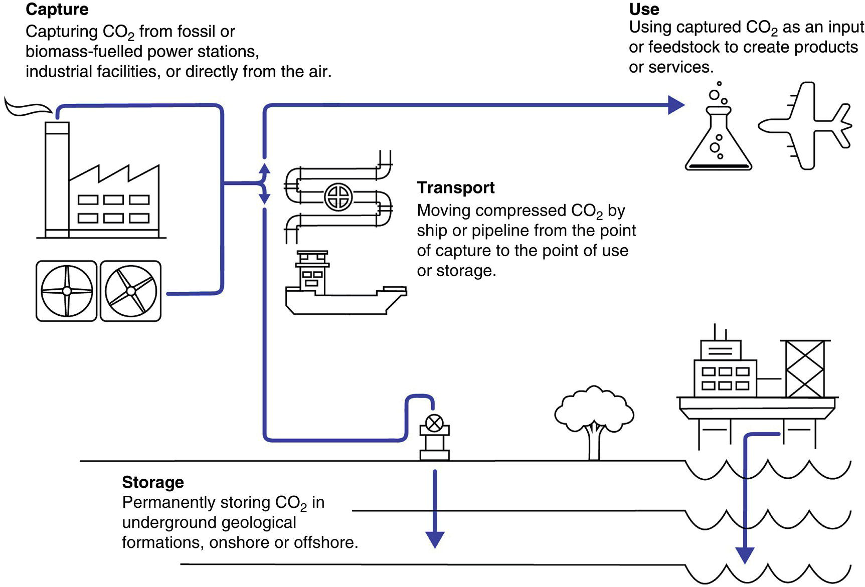
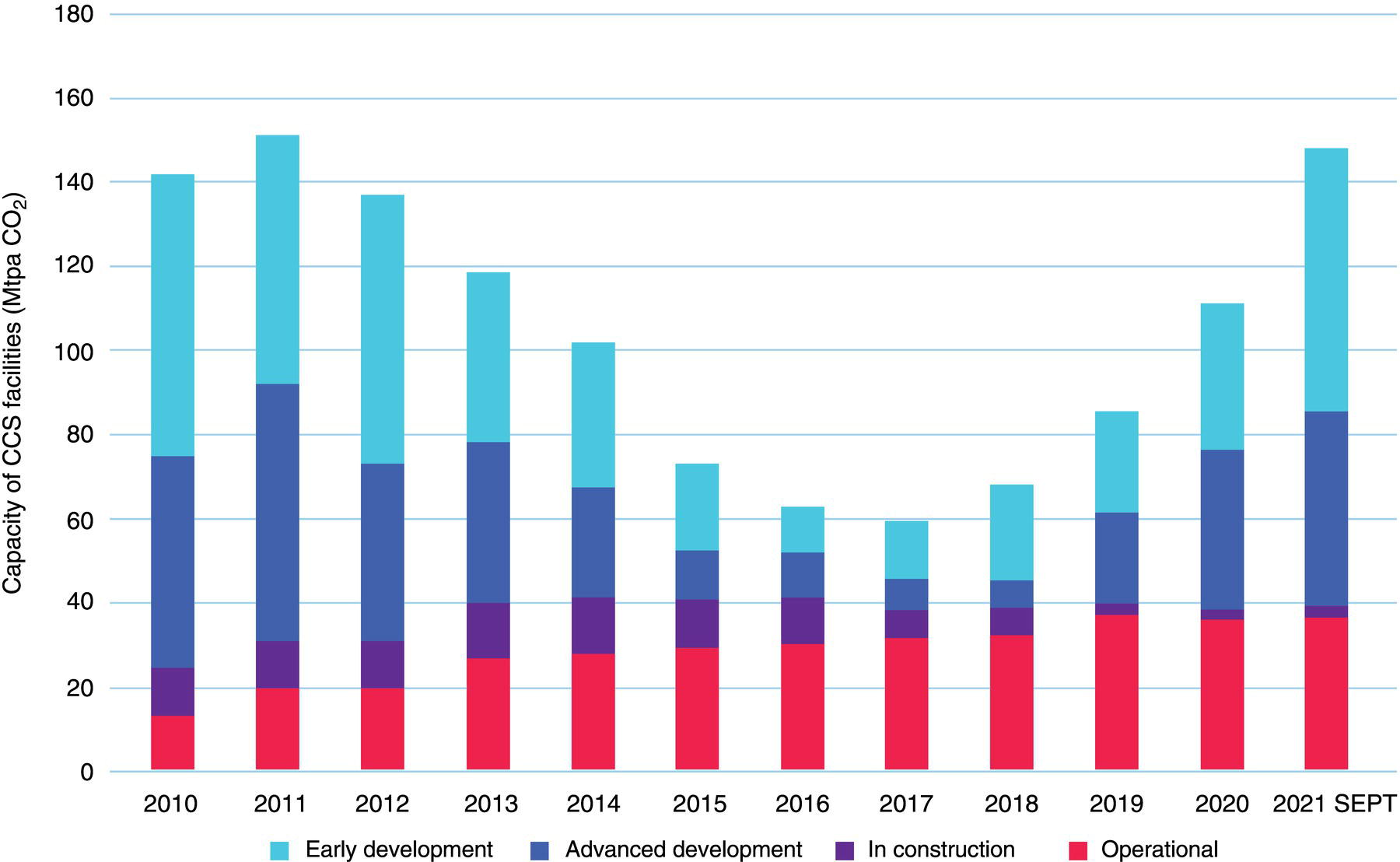
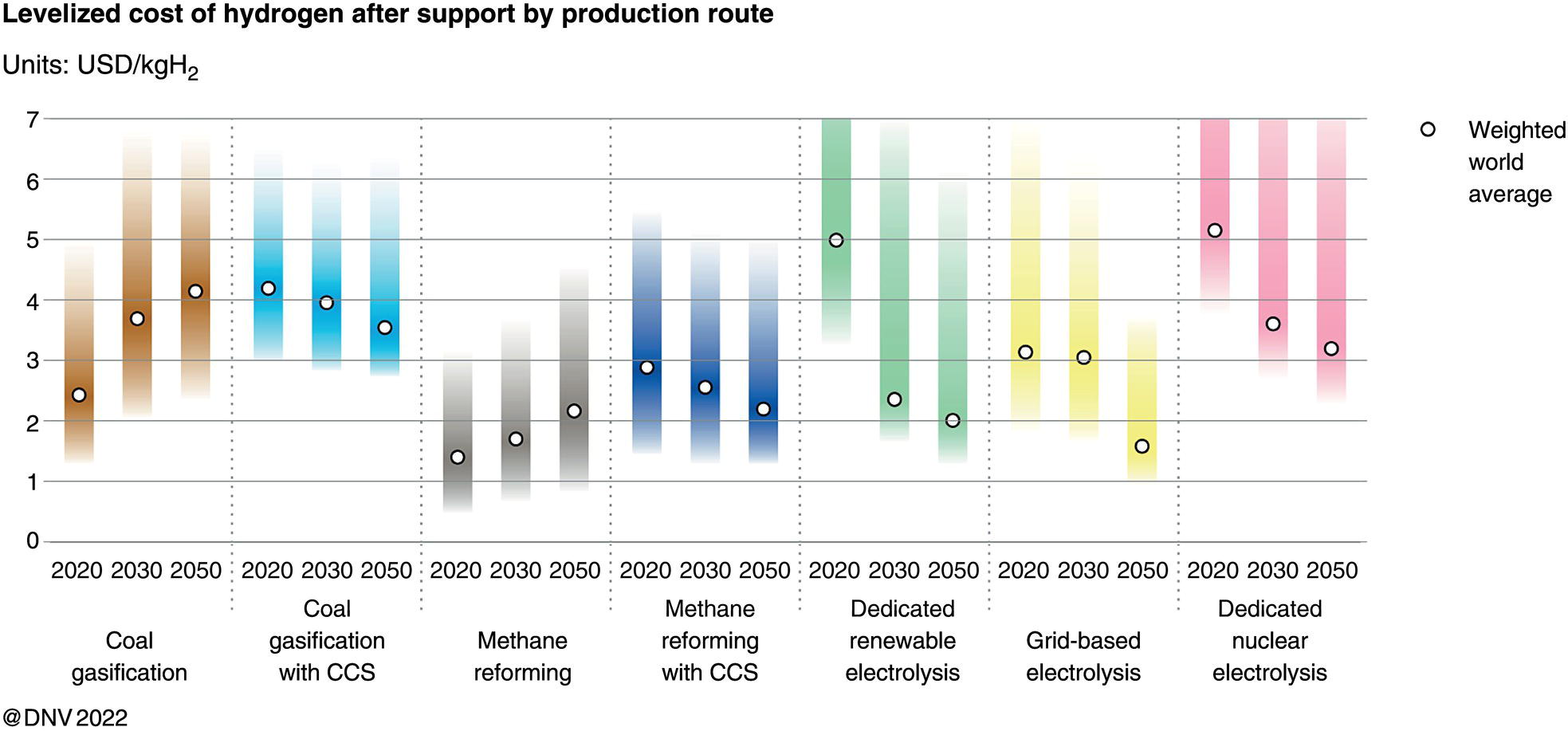
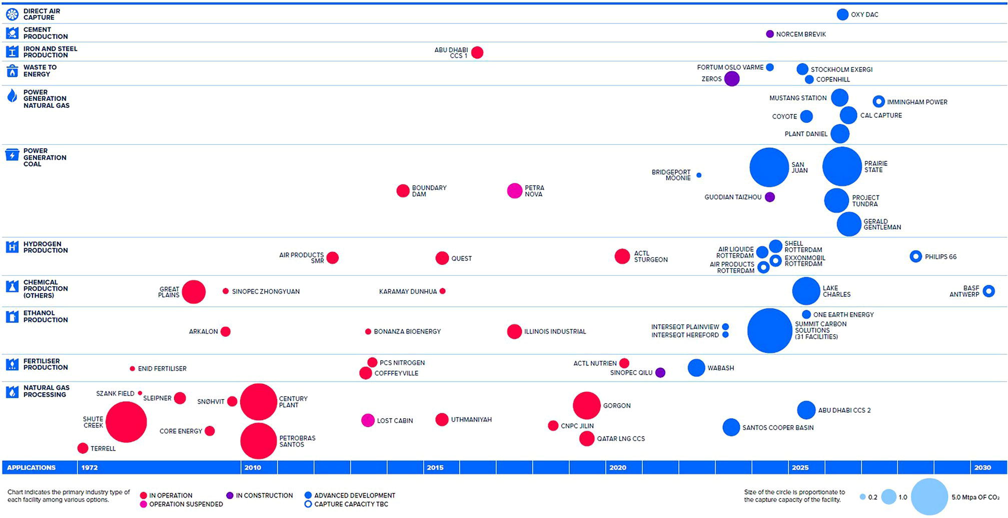
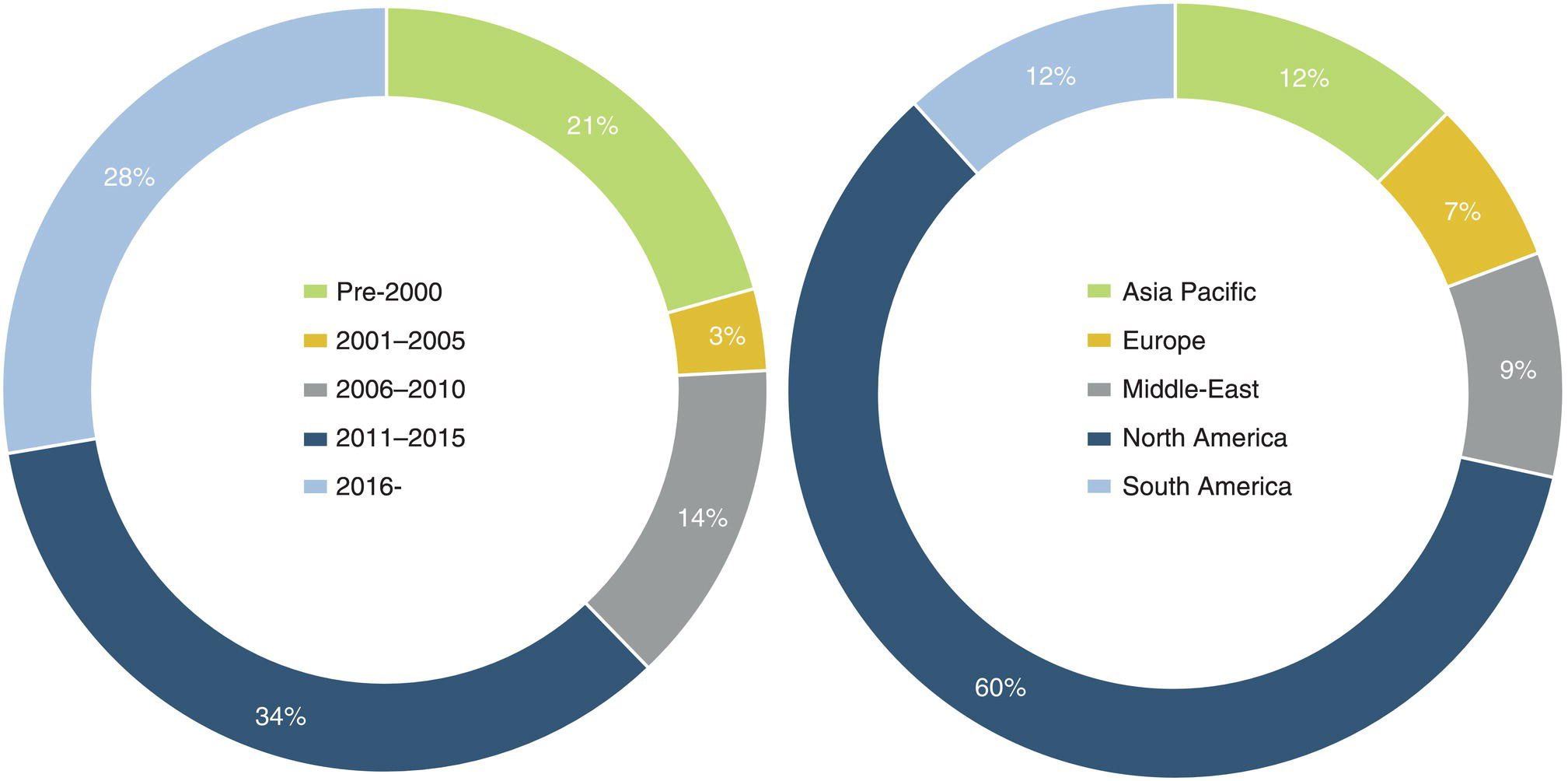
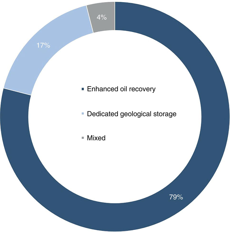
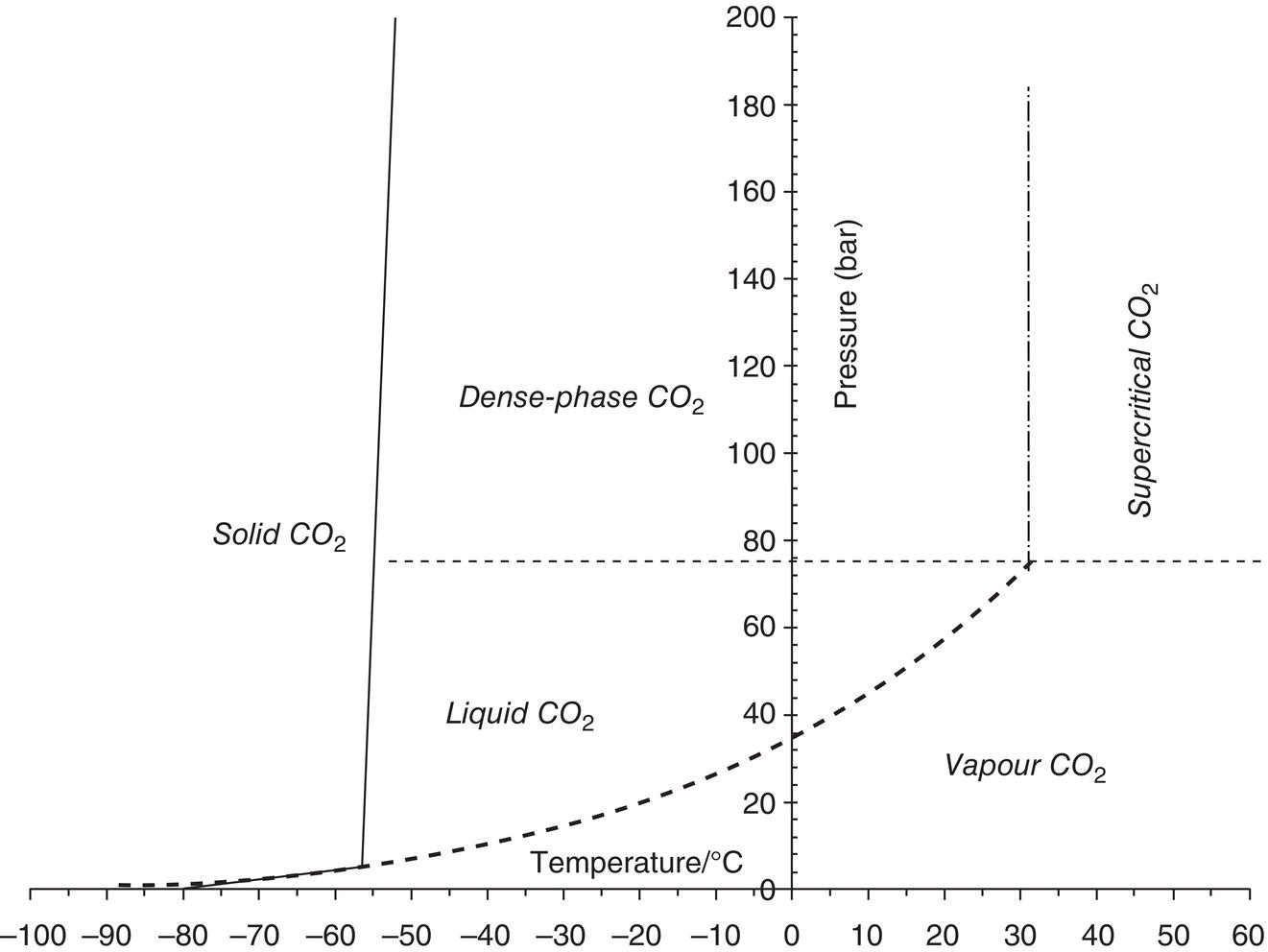
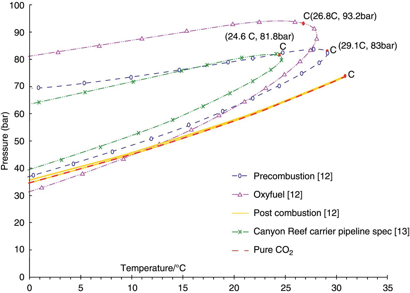
Daniel Sandana ROSEN (UK) Ltd., Newcastle upon Tyne, UK Since the COP 21 Paris Climate Conference in 2015, there have been strong incentives from global governments to tackle climate change and to drive the transition to a low-carbon economy. Currently,1 14 countries (mainly European but also including Canada, Japan, South Korea, and New Zealand) have legally binding net-zero emissions targets, and 32 (including the United States and China) have brought forward policy documents with targets. In almost all the rest of the world, the concept of net-zero is under discussion, and targets are being debated. Carbon capture, utilization, and storage (CCUS) is one prominent technology solution to achieve deep industrial decarbonization and reduce atmospheric CO2 emissions. It is “increasingly well placed to make a significant and necessary contribution to achieving net-zero emissions by 2050.”2 The deployment of CCUS at an industrial scale will require CO2 pipeline transportation, and the repurposing of existing hydrocarbon pipelines will play a major role in building this infrastructure. The transportation of CO2 entails its own pipeline integrity challenges. These need to be understood to safely manage CO2 pipeline operations and the conversion of existing hydrocarbon assets. This chapter introduces the necessity of CCUS as a key enabler of the global decarbonization agenda and discusses the current commercial status of CCUS worldwide. The landscape of CO2 pipelines (and their characteristics) worldwide is presented, and the importance of pipeline repurposing in the realization of the CCUS value chain is highlighted. As an essential facet of CO2 pipeline operations and integrity management, the key properties of CO2 are defined. Various CO2 compositions and impurities arising from different capture sources are reviewed, and the degree to which they could affect CO2 properties and operations is discussed. While reviewing the key pipeline integrity challenges pertinent to CO2 operations, the integrity management experience gained from operational CO2 pipelines is considered. The extent to which this knowledge remains applicable to the future of CCUS pipeline transportation infrastructure will be discussed. An important thesis of this chapter is that the conversion of existing hydrocarbon pipelines to CO2 service should be executed with due diligence and executed with the integrity threats posed by CO2 transportation in mind. Finally, key considerations and approaches for the safe repurposing of existing pipelines to CO2 transportation are presented in this chapter. Arising about 100 years ago, in the 1920s, the fundamental technologies behind carbon capture were developed due to the need to separate CO2 in natural gas reservoirs from salable methane gas. In the 1970s, this separation technology was taken a step further in Texas, as captured CO2 was piped to a nearby oil field and injected to enhance oil recovery (EOR). The idea of deliberately capturing CO2 for the primary purpose of removing it from the atmosphere was first introduced in 1977 [1], but it was only in 2005, at the G8 in Gleneagles, Scotland, that the leading governments formally acknowledged the need to develop carbon capture and storage (CCS) at an industrial scale to tackle climate issues: “We will work to accelerate the development and commercialization of CCS technology.”3 In 2007, David Cameron declared in China that “all existing coal-fired power stations should be retro-fitted with CCS, and all future coal-fired power stations should be built with CCS.”4 Yet, as of 2022, the story of CCS is one that has neither lived up to its promise nor fulfilled its hoped-for potential: Annual CCS investment has consistently accounted for less than 0.5% of global investment in clean energy and efficiency technologies [2], national government funding has collapsed between 2005 and 2015, and CCS infrastructure has a patchy record internationally. Figure 5.1 Schematic overview of the carbon capture, utilization, and storage concept. ([2]/IEA/CC BY 4.0.) Fundamentally, a key challenge is economics. Storing CO2 is a pure cost, and related investments have been limited, given the absence of regulatory incentives to defray the installation of capture technology and a storage infrastructure. Thus, the fact that the majority of existing operational CCS is being associated with EOR is not a surprise, but it does raise interesting questions about the net climate impact. One key path to looking at how carbon capture can be made more attractive financially would be to increase the value of CO2 as a feedstock for existing or new products through innovation and technology. Applications for captured CO2 can cover a wide range of materials, such as construction materials (cement), synfuels, and chemicals. It is actually interesting to see that this outlook has in recent years been integrated into the terminology of the capture chain value concept: No longer referring to CCS, the industry has now adopted the more profitable term of “carbon capture, utilization, and storage” (Figure 5.1) [2]. Despite the slow progress in development, there are clear signs that CCUS is gaining new momentum lately: There is increased policy ambition and action, more projects are coming online, and there are more plans to build new ones, as illustrated in Figure 5.2 [3]. One of the big factors driving this dynamic is the further realization that without CCUS, the energy transition and the 2050 net-zero objectives would become much more challenging. As of 2021, some 40 Mt of CO2 are captured and stored annually; it is estimated that this must increase 100-fold by 2050 to meet the scenarios laid out by the Intergovernmental Panel on Climate Change scenarios [3]. Aside from the manifest advantages of CCUS in achieving deep decarbonization, particularly in hard-to-abate sectors, the technology lately has also received greater interest owing to its role in enabling the realization of hydrogen at scale in the short-term. The deployment of a hydrogen economy is likely to rely heavily on the production of “blue” hydrogen (i.e., hydrogen generated from the steam methane reforming [SMR] process) over at least the next 10–20 years (i.e., 2030–2040)5 [4, 5]—until the production of green hydrogen becomes more economically competitive (see Figure 5.3). Some projections have estimated that about 2.5 Mt of blue hydrogen will be generated by 2030 [4]; this implies that a staggering 50 Mt of CO2 will be generated as part of the process, which will need to be captured, stored, or utilized. Figure 5.2 Overview of the capture and storage capacity of commercial CCUS facilities, 2010–2021 [3]. (Used with permission from Global CCS Institute.) Figure 5.3 Projected levelized costs of hydrogen by production route (as of 2022) [5]. (Used with permission from DNV.) Figure 5.4 Portfolio of CCUS commercial facilities worldwide as a function of power and industrial application (2021) [3]. (Used with permission from Global CCS Institute.) Figure 5.46 [3] illustrates the 2021 portfolio of CCUS commercial facilities, including those in operation, under construction, and in advanced development. In 2021, 27 commercial CCUS facilities were reported to be operational globally. Details of commercial facilities in operation are given in Table 5.1 [3]. As illustrated in Figure 5.5, the majority of these facilities have become operational in the last 10 years. CCUS assets are predominantly located in North America, while presence in other regions is scattered. Around 80% of the existing CCUS facilities are aimed at delivering EOR (Figure 5.6). Presently, there are over 8000 km of CO2 pipelines around the world. A list is detailed in Table 5.2 [6, 7]. The core of this infrastructure, approximately 90% of the pipelines, is located in the United States; pipelines moving CO2 are rare outside the United States. In the United States, the first large-scale CO2 pipeline, the Canyon Reef pipeline, was built in the 1970s. Much of the remainder of the current CO2 transportation infrastructure in the United States was built in the 1980s and 1990s. Even though US pipelines total approximately 7300 km in length, that figure remains low compared to the ~500,000 km of operational natural gas pipelines there. Overall, pipeline transportation is currently seen as a “weak link” in the CCUS value chain. The estimated CO2 transportation infrastructure to be built in the coming 30–40 years (consistent with the International Energy Agency’s least-cost pathway to cut energy-related CO2 emissions by half by 2050) is estimated to be a hundred times greater than what currently exists [8]. In North America alone, CO2 transportation is projected to need to reach around 45,000 km by 2050 [3]. Factoring the historical pace of CO2 pipeline construction—a rough average of 100 miles/year [6]—puts the scale of the challenge ahead into perspective. Finally, the building of the future CO2 pipeline transportation infrastructure will, to some degree, revolve around the repurposing of existing pipelines to overcome the cost and permit challenges associated with new pipeline construction. Repurposing a pipeline for CO2 service drastically reduces overall CCUS project costs (by up to 50–80%) and may, in fact, make the difference between the success and failure of a CCS project [9]. One clear example is offshore, where construction costs are prohibitively high; the industry will likely take advantage of existing pipelines for the geological storage of CO2 in depleted reservoirs, as is the case for several ongoing high-profile CCS projects in Europe, such as Hynet, Acorn, and L10. Table 5.1 Details of Commercial Facilities in Operation (2021) Source: Adapted from Ref. [3]. Note 1: Operations suspended. Figure 5.5 CCUS facilities by age (left) and regional capture capacity (right) (2021). (Daniel Sandana, ROSEN (author).) Figure 5.6 CCUS commercial facilities by storage type (2020). (Daniel Sandana, ROSEN (author).) The phase diagram for pure CO2 is illustrated in Figure 5.7 [10]. There are two distinctive features: the “triple point” (at 5.2 bar, −56 °C) and the “critical point” (at 74 bar, 31 °C). The curve linking these two points is the vapor–liquid equilibrium (VLE) line separating the gaseous phase and the liquid phase. Of importance: Table 5.2 List of CO2 Pipelines Figure 5.7 Phase diagram for pure CO2. ([10]/Reproduced with permission from ASME.) The most effective and economical manner of transporting CO2 by pipeline is in its supercritical or dense phase; this is of particular importance in storage applications. Gas phase transportation is not economically desired for long-distance transportation because of low density (and the ensuing requirement for larger diameters). In all but the shortest CO2 pipelines, the current operating practice for CO2 pipelines is to maintain pressure well above the critical pressure (and away from the VLE curve) to avoid the existence of a dual liquid-and-gas phase flow (which could lead to liquid slugs and compressor damage). Table 5.3 shows that long-transmission CO2 pipelines operate at a high maximum allowable operating pressure (MAOP) [11]. However, impurities can be present in the CO2 stream, particularly in the case of CO2 produced by human activities (referred to as “anthropogenic CO2” hereafter). These can induce important changes to the CO2 phase diagram, critical pressure and temperature, and hence to the operational envelope requirements to economically transport CO2 by pipeline [10]. This is discussed further in Sections 5.3.2 and 5.3.3. CO2 can be captured from natural sources as part of oil and gas production, as is currently the case for the majority of CO2 commercial projects in the United States. Or it can be of an anthropogenic nature, produced, for example, as part of power heat generation or, as discussed earlier, from SMR as a by-product of “blue” hydrogen. Whether CO2 is of a natural origin or human-generated, the stream will hold impurities—but the type and level are fundamentally dependent on the source. Table 5.3 MAOP for Long-Transmission CO2 Pipelines Table 5.4 Example of Compositions of CO2 Captured from Natural Gas and Transported in US Pipelines While CO2 captured from natural gases is often called “pure,” this is somewhat erroneous; the majority of the CO2 pipelines in the United States transport CO2 with impurities such as hydrocarbons, nitrogen, and water (Table 5.4) [12]. Nevertheless, CO2 streams directly generated from process plants tend to be richer in impurities and hold a wider spectrum of contaminants. Major impurities as function of the type of industry may be listed as follows (but not limited to): It is worth emphasizing that it is not possible, or at least challenging, to specify exact levels of impurities on a wider basis for various mainstream CO2 capture applications. The CO2 stream compositions will be affected not only by the type of industry and fuel source but also by project economics (increased capture cost associated with the removal of impurities to low levels) and geographies (local regulatory specification and safety requirements) [10]. An example of CO2 stream compositions from the three main CO2-capture power plant technologies (i.e., postcombustion, precombustion, and oxyfuel) are captured in Table 5.5 [13]. An example of a CO2 stream composition from an SMR plant (at Port Arthur) is shown in Table 5.6 [14]. As alluded to earlier, the introduction of impurities affects the phase behavior dictating the physical properties of CO2. The effect of impurities is generally that they lead to the formation of a wider dual-phase CO2 gas–liquid domain (Figure 5.8 [10]) and modulate the critical pressure and temperature. The extent of these changes and the direction of the trends are governed by the type, levels, and combination of impurities present. Seevam et al. [10] show, for example, that the addition of H2 and NO2 causes a larger increase in the dual-phase envelope, while other additions (e.g., N2 and H2S) may result in a much smaller increase. The addition of impurities also appears to increase the critical pressure while decreasing the critical temperature (except for NO2). Table 5.5 Example of Impurity Combinations from Main CO2-Capture Power Plant Technologies Table 5.6 Example of CO2 Compositions from a Steam Methane Reforming Plant (Port Arthur) a Average values; actual CO2 percentages from approx. 96.00–99.50% over the 24-h test. Seevam et al. [10] have also simulated the variations in CO2 phase behavior for some impurity combinations from the main CO2-capture power plant technologies and from the Canyon Reef pipeline specification. The following observations were made (Figure 5.8 [10]): Figure 5.8 Phase diagram of the impact of impurities on CO2; comparison of the three different capture streams and the Canyon Reef pipeline specification. ([10]/Reproduced with permission from ASME.) While these trends are interesting in their own right, it is important to appreciate that they are only representative of the selected compositions and mixtures. Other mixtures and compositions could be present in the pipeline, depending on the respective project stream specifications. As mentioned before, it is more beneficial from an efficiency and economical perspective to transport CO2 in the dense phase. Although transportation in the gas phase is feasible, it is not ideal for pipelines of any significant capacity and length. In addition, two-phase flow in pipeline transportation should be avoided to prevent liquid slugs and potential damage to the pipeline and associated equipment. Therefore, the target is to maintain the pressure well above the critical pressure in the pipeline. We discussed that the addition of impurities can greatly influence the critical point, with some having the potential to increase the critical pressure. A direct consequence of this is that the presence of impurities affects many aspects of CO2 pipeline transportation, especially the determination of the optimum operating pressures, pipeline sizing, repressurization distance, and the number of pumps and their power requirements [10]. The effect of impurities on repressurization distance is of particular concern for offshore pipelines. It is therefore essential to study, on a case-by-case basis (depending on the respective project CO2 specifications), the impact of the expected combination of impurities on the formation of two-phase regions in the CO2 phase diagram and on the critical pressure and temperature, to ensure that the pipeline is operated outside the dual-phase CO2 gas–liquid region. The evaluation of these influences is also very important when it comes to determining the pipeline material property requirements (fracture toughness) for safe CO2 transportation; this is further discussed in Section 5.4.2. There are a multitude of damage mechanisms applicable to any in-service pipelines—irrespective of the nature of fluids transported—that need to be tackled as part of general pipeline integrity management practices. For example, these can include external interference (third-party damage), external corrosion, and geohazards. Section 5.4.1 only addresses internal time-dependent threats directly induced by the transportation of CO2. Once these threats are understood, the plausible modes of pipeline failure need to be considered. A particular concern for the operation of dense-phase CO2 pipelines is fracture control to manage the risk of ductile fracture propagation (Section 5.4.2). Figure 5.9 Solubility of water in pure CO2 as a function of pressure and temperature. (From Project Internal Memo, DYNAMIS: Inert components, solubility of water in CO2 and mixtures of CO2 and CO2 hydrates, by A. Austegard, and M. Barrio, Trondheim, Norway, 2005. © SINTEF Energy Research. Used with permission from SINTEF.) In many respects, the management of internal time-dependent threats in CO2 pipelines is fundamentally an extension of the knowledge and experience gained from the traditional oil and gas industry. The main key difference is that in “traditional” gas production, CO2 is mainly an unwanted by-product or impurity, while for CCUS, CO2 is the primary fluid being transported. Hence, it will likely be at a higher partial pressure (which will broadly speaking mean a greater corrosion risk) and may have its own inherent impurities. For oil and gas infrastructure, it is generally accepted as a simplified rule that the risk of internal corrosion in transporting facilities will remain low as long as no free (separated) water phase is present [15, 16]. Broadly speaking, if the water remains dissolved in the hydrocarbon phase, whether it is in a gas or a liquid phase, the formation of acids (due to the dissolution of CO2 or H2S in liquid water) responsible for sweet and sour corrosion mechanisms is not possible. By extension, this means that an effective mitigation of internal time-dependent threats for CO2 pipelines is to use dehydration processing to keep the water content below saturation levels or its solubility limits in the CO2 stream. The latter is a function of the operating pressure, operating temperature, and, not least, of the type and amounts of impurities present [17, 18]. Figure 5.9 [19] illustrates the water solubility in pure CO2 as a function of pressure and temperature. It can be seen that: An acceptable water specification for avoiding corrosion in pipelines transporting pure CO2, at operating temperatures above 4 °C, is generally considered to be in the range from 300 to 500 ppm wt (0.4 kg/m3 or 0.0003–0.0005 ppmv) [19, 20]. Nonetheless, the former is only valid for pure CO2; once more, the influence of impurities needs to be considered. Water solubilities could be affected and decreased depending on the type, concentration, and combination of impurities. For example, Austegard et al. [18, 21] showed that CH4 will lower the solubility of water in CO2, which is also potentially the case for other impurities, e.g., N2 and HCl [22, 23]. Similarly, and of particularly great importance for anthropogenic CO2 from power plants, the presence of sulfur oxides (SOx) and nitrogen oxides (NOx) can drive the formation and drop-out of acid aqueous phases at water contents much lower than the water solubility limit in otherwise pure CO2 streams. This is related to the formation of weak and strong acids, i.e., H2SO3, H2SO4, and HNO3, at a temperature much higher than the water dew point, which is commonly referred to as the acid dew point [24–28]. For example, the impact of SO3 on the acid dew point in combustion gas condensates is illustrated in Figure 5.10 [29]: when the concentration of SO3 in the gas is increased, the acid dew point temperature increases (the presence of SO2/SO3 react with water vapor to form sulfurous or sulfuric acids). It is noted that, while the formation of sulfurous and sulfuric acids can form in the presence of SO2, Morland [30] and Sonke [31] indicate that the presence of SO2 only in the CO2–H2O–SO2 system does not appear to have a significant influence in the formation of a separate acid phase (even in the presence of oxygen) under dense CO2 transportation conditions, due to the necessity of high reactant concentration limits for acid formation and dropout, and also potentially low reaction kinetics. The additional presence of NO2, however, plays a strong catalytic role in the formation of H2SO4: The reaction H2O + SO2 + NO2 leads to the formation and dropout of H2SO4 at much lower concentrations of SO2 (compared to H2O + SO2 or H2O + SO2 + O2). Figure 5.10 Variation of sulfuric acid dew point for gases having different water vapor contents as a function of SO3 levels. (Used with permission from Emerald Publishing Limited from Ref. [29]; permission conveyed through Copyright Clearance Center, Inc.) The formation of strong acids in reasonable timescales (kinetics), of importance sulphuric acid, has been reported to be the result of concomitant reactions involving multiple impurities in the balance, particularly NOx, SOx, O2, H2S. Sonke and Zheng [31] have reviewed the most likely chemical reactions that may occur between typical impurities (H2O, SO2, NO2, H2S, O2) in the development of a separate acid phase; a summary has been compiled in Table 5.7. As discussed before, the strong oxidizing agent NO2, and to a lesser degree H2S, drive the most of the reactions leading to the formation of an aqueous phase containing H2SO4 and HNO3. If NO2 or H2S are absent, the formation of strong acids will not occur in practical times, or necessitates higher concentrations of reactants. It is essential that CO2 transport specifications are derived such that considered levels of water and impurities do not lead to the formation and dropout of a separate corrosive acid phase (and solids). It is then necessary to have a thermodynamic model that can predict both phase and chemical equilibria in in the CO2-rich phase and the water-rich phase. The use of mixed- solvent electrolyte (MSE) model, which has been designed in the γ−φ framework7 for the simultaneous calculation of phase and chemical equilibria in systems containing strong and weak electrolytes in aqueous, nonaqueous, and mixed solvents, has been discussed to provide a suitable foundation by Morland and Springer [32, 33]. It is nonetheless emphasised that a key limitation is that this model, albeit being a valuable screening tool, is thermodynamics-based, and does not consider kinetics – Whether reaction will actually take place or how fast? Another key point is that H2SO4 (and elemental sulphur) has a low solubility in dense phase CO2, while HNO3 has a relatively high solubility. The implication is that for corrosion control, the preferred option would be to prevent the formation of H2SO4, while for HNO3 the preferred option would be to avoid drop-out. The main internal threat is CO2 corrosion, commonly referred to as sweet corrosion. The key parameters driving the magnitude of the corrosion growth are (1) water content in the CO2 stream, (2) volume of water separated and exposed pipe-surface-to-water volume ratio, (3) CO2 pressure (fugacity), (4) type and partial pressure of impurities (and combination), (5) temperature, (6) flow, and (7) duration of the water dehydration upset condition (exposure time). Pure CO 2 –H 2 O A great deal of research has been published over the last decade to quantify the rates of uniform and pitting corrosion that could be expected in pure CO2 pipeline service. Table 5.7 Summary of Most Likely Chemical Reactions Between Impurities for the Formation of a Separate Acid Phase in Dense CO2 Source: Data from [31]. Table 5.8 Summary of uniform corrosion rates of steels exposed to a water-saturated and undersaturated dense CO2 phase Tables 5.8 and 5.9 provide a summary of experimental uniform and pitting corrosion rates of steels exposed to a water-saturated and undersaturated dense CO2 phase. Table 5.8 indicates that uniform corrosion rates are relatively low under these conditions. Table 5.9 indicates that the reported experimental pitting corrosion rates are much higher irrespectively whether the supercritical CO2 phase is undersaturated or saturated with water. It is however highlighted that corrosion rates reported in dense CO2 phase for water concentrations well below the saturation limit should be considered with due caution: Morland and Svenningsen [41] indicates that these could be associated with pitfalls and artifacts in experimental procedures; the authors suggest the corrosion rates should be low (<0.001 mm/year) as long as the water is fully dissolved in the CO2 phase. In cases where significant dehydration upsets occur, and a free water phase is present in the dense CO2 transport pipeline, most sources agree that excessive uniform corrosion rates are expected in the CO2-saturated water phase (much higher than the water-saturated supercritical CO2 phase as reported in Table 5.8). This is shown in Figure 5.11 [35–39, 42, 43] and Table 5.10; note the scatter in reported experimental corrosion rates between sources is considerable (generally from 1 to 40 mm/year in pure CO2), and it can be explained by differences in experimental protocols and test conditions, e.g., CO2 pressure, temperature, pH, flow conditions, but also exposure time. The corrosion rate in the CO2-saturated water phase is expected to decrease with exposure time (i.e., in the case of nonreplenishing free water dropout conditions) due to the formation of partly protective films and as illustrated in Figure 5.12 [16], albeit high corrosion rates could be sustained for a substantial time (more than few days) prior to decreasing [48, 55]. For example, Dugstad et al. [36] reported corrosion rates of 3–6 mm/year after few days of exposure, in water phase in equilibrium with dense-phase CO2 (100 bar) under dynamic flow conditions (1–3 m/s) and a temperature of 13 °C. Table 5.9 Summary of Pitting Corrosion Rates of Steels Exposed to a Water-Saturated and Undersaturated Dense CO2 Phase Figure 5.11 Comparison of experimental uniform corrosion rates of steels reported in dense CO2-saturated water phase versus water-saturated-dense CO2 phase. (Daniel Sandana, ROSEN (author).) Presence of impurities. As discussed in Section 5.4.1.1, the presence of impurities such as H2O, SO2, NO2, H2S, and O2 have the potential to participate in cross-chemical reactions and produce sulfuric/sulfurous acid, nitric acid, and elemental sulfur; these can form separate acid aqueous phases and contribute to corrosion at water contents much lower than solubility limits in pure CO2. Cross-chemical reactions. Combinations of impurities that can lead to corrosion during dense CO2 transportation shall be avoided. Experimental corrosion rate data of steels exposed to dense CO2 and containing impurities have been compiled from existing literature for the following systems: Table 5.10 Summary of Corrosion Rates of Steels Exposed to a Free CO2-Saturated Water Phase Figure 5.12 Comparison of a sample of published corrosion rates in pure CO2-saturated water phase (10–100 bar) and impact of exposure time. (Daniel Sandana, ROSEN (author).) As a point of caution, it must be noted that many of these experiments were conducted with autoclaves (closed systems) without replenishment of impurities over testing duration. Since the impurities are tested at low concentrations, they may be consumed in a short space of time in corrosion processes, and the effect of the considered impurities may be overall underestimated. The following observations may be made; the effect of impurities is further discussed in Section 5.5.1 and Table 5.20: Single impurities in dense CO 2 Presence of FeSO3 and/or FeSO4 on the corroded surface in some experiments indicate that the reactions occur at water concentrations far below the water solubility in the pure CO2–water systems. Table 5.11 Summary of Corrosion Rates of Steels Exposed to a Dense CO2 Phase Containing Water and SO2 a Caution to be considered due to experimental protocol used. Table 5.12 Summary of Corrosion Rates of Steels Exposed to a Dense CO2 Phase Containing Water and NO2 a Caution to be considered due to experimental protocol used. Table 5.13 Summary of Corrosion Rates of Steels Exposed to a Dense CO2 Phase Containing Water and H2S Table 5.14 Summary of Corrosion Rates of Steels Exposed to a Dense CO2 Phase Containing Water and O2 a Caution to be considered due to experimental protocol used. Table 5.15 Summary of Corrosion Rates of Steels Exposed to a Dense CO2 Phase Containing Water, SO2, and O2 Table 5.16 Summary of Corrosion Rates of Steels Exposed to a Dense CO2 Phase Containing Water, NO2, and O2 Table 5.17 Summary of Corrosion Rates of Steels Exposed to a Dense CO2 Phase Containing Water, SO2, and NO2 Table 5.18 Summary of Corrosion Rates of Steels Exposed to a Dense CO2 Phase and Water, SO2, NO2, H2S, O2, and CO Multiple impurities in dense CO 2 It is emphasized that corrosion rates in a CO2–water-saturated phase (in the presence of impurities) are expected to be significantly higher than those quoted in Tables 5.11–5.18. They are also expected to be higher than those reported for a pure dense CO2–H2O system due to acidification (lower pH) and destabilization of protective films by impurities such as NO2, SO2, and O2. It is generally held that the presence of CO2 alone (in the presence of free water) is not sufficient to drive the initiation and propagation of stress corrosion cracking (SCC). However, in the presence of a separate aqueous phase, there could be specific stress conditions for which SCC can be observed. For example, Hudgins et al. [69] indicate that cracking may be generated on high-strength carbon steel in high-pressure CO2 environments under extreme stress conditions with relatively long exposure times. At 20 bar, CO2 failures were produced during exposures of as low as 22 h on steel materials with a hardness of 34 HRC/320 HV and deformation levels of 115%; the production of cracks was associated with the potential leaching of sulfur from the steel materials. CO2-H2O SCC is a mechanism that has also been practically identified as a failure mode in flexible armors [97]. The phenomenon has been observed to take place notably in severe CO2 environments and high applied stresses (equivalent or over to 100% SMYS) and is a cause of great concern to the flexible pipe industry. Although these hardness and strain levels are significantly higher than those that would be found in most pipelines, scenarios should be considered where such high stresses (e.g., from geological ground motion) and high-hardness materials (e.g., hard spots) may arise. The potential presence of CO and H2S in CO2 streams (e.g., in CO2 streams derived from precombustion or SMR processes) also implies that certain specific environmentally assisted cracking threats may need to be considered [75] in the presence of an aqueous phase, namely CO2–CO–H2O SCC [76, 77] and sour (H2S) cracking [78]. The presence of H2 can also lead to hydrogen embrittlement/hydrogen-environmentally assisted fatigue. There is a fundamental requirement to obtain data at high partial pressures of CO2 and dense CO2 conditions to discuss further the susceptibility to these threats in CO2 transportation service, and define acceptable impurity limits. Some may question whether crack initiation may be practically feasible in a CO2 pipeline due to the severity of internal corrosion once water condensation occurs. Nonetheless, some industry cases indicate that these mechanisms should not be overlooked. An example of the interaction between sour service and supercritical CO2 may be found in the Tupi field offshore Brazil. In this case, Petrobras recently decided that rigid risers featuring titanium stress joints and ruthenium alloys were required to mitigate the risk of SCC [74]. In the 1970s, cracking of carbon steels was observed in environments constituted of wet mixtures of carbon dioxide and carbon monoxide gases, such as those present in coal chemical processing plants, and town-gas manufacture, transport, and storage systems. Brown et al. [77] and Kowaka and Nagata [76] showed that transgranular SCC is possible in the CO2–CO–H2O system. The mechanism is induced by stress, the presence of liquid water, and CO activity. The additional oxygen increases the susceptibility of SCC by shifting the free corrosion potential in the domain of SCC initiation, and increasing propagation growth rate. The mechanism of SCC for the CO2–CO–H2O system has been classed under the “strain-generated active path” model: a monomolecular CO film is formed on the surface of the carbon steel and ruptures under stress; local anodic attack ensues, and the cycle of events repeats [79]. Most of the experimental data are limited to low partial pressures of CO2 (<20 bar). More recently [70], a X65-pipeline steel was tested by four-point bend test at 50 bar CO2 in the presence of 1000 ppm CO. The steel specimens were submerged in water, and no cracking was identified. Further experimental testing at high CO2 partial pressures typical of gaseous and dense CO2 conditions is needed. The presence of H2S can lead to different types of sour cracking, mainly sulfide stress corrosion cracking (SSCC) and hydrogen-induced cracking (HIC). These threats and their respective mitigation requirements have been well documented in the oil and gas industry, especially through the standard NACE8 MR0175/ISO 15156 [78]. As water upsets should be ideally minimized in CO2 transportation operations, HIC should not be expected as the mechanism is a rather slow process, which may not be the case for SSCC. While some have considered that NACE MR0175/ISO 15156 remain applicable for evaluating SSCC, there are some major short falls to consider, that impact [31] its use for dense CO2 transportation. Key inputs in the aforementioned NACE/ISO standard are H2S partial pressure (pH2S) and pH; however: Further work is ongoing to identity safe limits for H2S in CO2 transport in regards to sour cracking issues. Note: NO2 reacts with H2S to form SO2; this reaction can effectively lower the content of H2S in the water phase and thus reduce sour crack threat. However, to take the benefit of this, a minimum NO2 concentration will be necessary, which is not practical and safe. Molecular hydrogen may dissociate into atomic hydrogen, which can then be adsorbed and diffuse into the steel lattice. The presence of atomic hydrogen in the lattice can lead to embrittlement. This can be practically translated into (i) degradation of toughness, which impacts on the tolerance of cracks, and (ii) fatigue crack growth of preexisting flaws under dynamic loading. While data on this topic remain sparse, Sonke and Zheng [31] suggest that the presence of H2 is expected to have minimal impact on the fracture toughness, due to expected low concentrations in dense CO2 transportation. The author believes this can be misleading as research on pipeline integrity in gaseous hydrogen blends shows that initial decrease in fracture toughness can be very significant at small amounts of hydrogen. For example, Kuo et al. reported a noticeable drop in initiation fracture toughness (KJth) in CO2 and H2 blend conditions compared to the inert test conditions [98, 99]. Further testing is required. Thodla et al. [80] investigated the impact of hydrogen on fatigue crack growth rates (FCGRs) in dense CO2 for the following conditions: 2 bar H2 and 100 bar CO2. It was reported that albeit FCGRs are multiplied by a factor of 10 compared to in-air conditions at high ΔK, the behavior is comparable to the fatigue design basis used for offshore pipelines subject to nonsour service or that of FCGRs in seawater under sacrificial cathodic protection. At low ΔK, the FCGRs at 2 bar H2 and 100 bar CO2 are significantly lower. Sonke and Zheng [31] concluded that an impurity limit of up to 1% H2 (equals 2 bar H2 in 200 bar operating conditions) seems therefore an acceptable limit for which pipeline design does not require specific adjustments. Higher concentrations of H2 require further testing before acceptance in a CO2 specification. The principal concern regarding the required mechanical properties of CO2 pipelines is generally considered to be related to the control of fracture propagation, and particularly to how a long-running ductile fracture can be prevented (or arrested) [81–83]. The means of averting the propagation of ductile fractures are conceptually relatively simple. One consists of specifying a line pipe with a sufficiently high toughness requirement (i.e., a minimum upper-shelf Charpy V-notch [CVN] impact value). A second method exists and entails the fitting of mechanical crack arrestors in regular intervals along the pipeline length. However, retrofitting crack arrestors on existing facilities is costly and does not assure shorter fracture lengths; this makes this alternative, the least preferred. In addition to the issue of long-running ductile fractures, the possibility of long-running brittle fractures should also be considered. Historically, brittle fracture has been mitigated by means of drop wear tear test (DWTT) requirements on the parent material. Fracture control is not a new concept for pipelines, and the normative Annex G of API 5L specifies additional provisions that can be applied. But, there are drawbacks in trying to apply these requirements to the repurposing of lines for CO2 transport. First, there is no guarantee that Annex G will have been applied to the pipeline at the time of construction (not least because Annex G is specifically for onshore buried gas pipelines, while some pipelines due to be repurposed may be offshore or originally in liquid service). Second, the requirements for fracture control in CO2 differ from those in natural gas, as discussed in the following. CO2 pipelines are more susceptible to long-running ductile fracture (than natural gas transportation) because the CO2 is transported in its dense phase and, more importantly, because of the specific decompression behavior of dense CO2 to a two-phase mixture. Broadly speaking, and as conceptualized by the widely used semiempirical Battelle two-curve model (TCM) [84], a ductile fracture will continue its propagation if the fluid decompression acoustic velocity (energy-driving force) is equal to or lower than the fracture propagation speed (resistance to the crack propagation). Figure 5.13 illustrates a simplified version of the TCM as applied to CO2 compared to natural gas. If we consider rupture in CO2 and natural gas (NG) pipelines [85], the initial speed of sound in CO2 is significantly greater than in NG. However, in the case of CO2 (as opposed to NG), there is a clear discontinuity and the establishment of a long plateau10 at a pressure [71] referred to as the saturation pressure,11 which is associated with the crossing of the two-phase liquid–gas boundary. The plateau extends down to low decompression velocities, which means that at a given fracture velocity, the pressure at the crack tip will equalize at the saturation pressure, and ductile propagation will ensue. Figure 5.13 TCM schematic showing decompression speed for CO2 and NG relative to fracture propagation speed. A key implication of this is that the arrest pressure,12 which is the pressure below which a running ductile fracture cannot be sustained, can be described (conservatively) as the saturation pressure in the case of a CO2 pipeline [84]. Accordingly, the saturation pressure must be less than the arrest pressure of the pipe to arrest ductile fracture propagation. For perspective purposes, the saturation pressure for a typical dense CO2 pipeline is 70 barg, while the design pressure for an NG pipeline is typically 75 barg. This means at lower acoustic velocities, the pressure at a given decompression wave velocity will be much greater for a CO2 line (i.e., the saturation pressure) than that of an NG line. This ultimately implies that a higher toughness would be required to arrest a ductile running fracture in a dense-phase CO2 pipeline than in a NG line. The high “saturation pressure” and the low decompression velocity across the two-phase region are the reason why a higher toughness is required to arrest a propagating ductile fracture in a CO2 pipeline than in an NG one [86]. While the principles for arresting a ductile running fracture notionally appear easy, the complexity lies in determining the actual minimum toughness that is required to arrest a ductile fracture for a dense CO2 pipeline. The established model for predicting the arrest toughness for natural gas pipelines is the TCM model. As this model was originally validated through a range of full-scale tests on lean and rich gases, the pertinence of its application for dense CO2 lines needed further evaluation through full-scale fracture propagation testing. Table 5.19 Summary of BS EN ISO 3183/API 5L PSL 2 and Project-Specific CO2 Transmission Charpy V-Notch (CVN) Impact Energy Requirements a Increase impact energy requirements in square brackets for pipe >762 mm nominal diameter up to 1219 mm diameter and grades up to X65. b Based on Table G.2, design factor of 0.72, 914 mm OD, X65/L450. Various evaluations [72, 85, 87, 88] reached a similar consensus, namely that the TCM is nonconservative and cannot be (currently) applied to dense CO2, even with the use of some notionally conservative correction factors, as propagation was observed at levels of toughness equal to or higher than that predicted by the model. This, in turn, means that existing material specifications, and indeed existing pipelines that have been proven by theory and experience to be resistant to ductile fracture propagation over many years of hydrocarbon service, may not be resistant in CO2 service. The evaluation raised some interesting questions [85], including: Why is the two-curve model nonconservative? Why is the driving force higher (if it is indeed higher)? Why is the initial speed of the expansion wave slower than predicted? Why is the plateau in the decompression curve a sloping plateau?13 The discrepancies compared to the predictions may find a reasonable justification in that, at high CVN values, it can be difficult to separate out the relative contributions of resistance-to-fracture initiation compared to propagation; hence, the resistance to propagation could not be accurately quantified. Alas, this explanation may not offer the complete resolution to the problem [85]. Nonetheless, a somewhat more positive outcome was reported in the case of the 2016 UK Yorkshire and Humber CCS cross-country pipeline project. The review of the dataset of two initial “failed” tests contributed to the successful prediction of an adequate arrest toughness during the execution of a third (and final) test, i.e., 250 joules (J) at a maximum saturation pressure of 80 bar, thanks to the use of additional corrections [85]. The investigators hint at the foundation of an empirical correlation, but further quantification would require additional full-scale testing data. It is generally acknowledged that more full-scale testing data will be welcome to assist with the development of more suitable empirical arrest toughness models. The lessons of the aforementioned third test were integrated in the Yorkshire and Humber CCS pipeline specification; an average CVN of 250 J was required for the line pipe body, but as alluded to before—and not least—this assumes a maximum CO2 saturation pressure of 80 bar. The project-specific Charpy requirements are shown in Table 5.19, with the equivalent values for “standard” API PSL 2 pipe and Annex G requirements shown for comparison. As can be seen, there are no significant differences in the Charpy requirements for welds (reflecting that long-running ductile fractures purely through seam welds are impossible, as they will eventually be arrested by the pipe body material in the downstream joint). However, the body Charpy requirements are significantly higher than either PSL 2 or Annex G requirements. This discrepancy means that the repurposing of existing pipelines with material originally specified to be in accordance with PSL 2 or Annex G can be challenging.*** As has been alluded to before, that 250 J above can be seen on some level as a default minimum CVN criterion to tackle ductile fracture propagation. This 250 J value is essentially empirical, and therefore there is reason to believe it is conservative and that additional tests may offer the opportunity to reduce it slightly. However, an important caveat suggested by the Yorkshire and Humber CCS line pipe test program is that the CO2 saturation pressure should not be higher than 80 bar. It was indeed demonstrated that long ductile fracture propagations are possible on high-toughness steels (with a specified minimum CVN of 250 J) at higher saturation pressures [88]. Fundamentally, the susceptibility to long-running ductile fractures increases with the saturation pressure [83]. As saturation pressures rise, higher arrest pressures, and thus higher fracture toughness (or thicknesses), will be required. Calculating the saturation pressure of the CO2 mixture is therefore an important input for controlling ductile fracture propagation. It is also paramount to appreciate the influences of the presence, nature, and levels of impurities in CO2 on the saturation pressure, and thereby on the toughness requirements. It was indeed discussed [83, 84] that the presence of certain impurities will increase the saturation pressure, with the impact growing in the following order: methane < oxygen < carbon monoxide < nitrogen < hydrogen. In general, it has been pointed out that the impurities that increase the saturation pressure are those with a lower critical temperature than CO2; Figure 5.14 [89] illustrates these. In the case of SMR-generated CO2, available compositions at Port Arthur indicate that H2, N2, CH4, and CO will be present in the mixtures; it may then be expected that for such streams, more stringent fracture toughness requirements may be necessary. Nonetheless, this needs to be fully quantified on a case-by-case basis against applicable compositions and specifications. For the purpose of converting existing hydrocarbon pipelines, this could mean that a backward-engineering approach would need to be undertaken, and the requirements of a quality (entry) specification and operational envelope will need to take into account the repurposed pipeline construction “DNA” (i.e., toughness, grade, diameter, thickness) for fracture control. Finally, it is worth observing that the composition of the CO2-rich mixture is a key influencer of saturation pressure—but so is the initial operating pressure and temperature of the CO2 line before a scenario of loss of containment. It was discussed in detail by Cosham [84, 86] that the saturation pressure increases with decreasing initial pressure, on the one hand, and with increasing temperature, on the other, the effect being greater playing with the temperature. Lower temperatures also increase hydraulic and thermal efficiency. As mentioned earlier, there are approximately 7300 km of pipeline operating dense CO2 in the United States. More than 40 years of practical experience has been gained, making it interesting to review what the industry experience has been from an integrity management perspective. In the first instance, the US experience regarding dense CO2 transportation has been positive overall. The number of reported incidents for these pipelines has been relatively low. The annual number of incidents per km was 0.0010/km/year in 1972, and it dropped to below 0.0002/km/year in 2002. Most of the incidents were associated with very-small-diameter pipelines (less than 100 mm in diameter); the failure incidents for 500 mm and larger pipelines were reported as much lower, below 0.00005/km/year. Between 1986 and 2006, the incident rate was as low as 0.0003/km/year for CO2 pipelines in the United States. Of interest, corrosion was not the major factor in these leaks [90]. The corrosion rate in an operating dry supercritical CO2 pipeline was reported at between 0.25 and 2.5 μm/year over 12 years of operation [91]. Figure 5.14 Relative critical pressure and temperature compared to CO2. ([89]/Reproduced with permission of J.M. Race.) To the author’s knowledge, no in-service long-running ductile fracture propagation incident has been reported. While the US experience provides practical proof that CO2 pipelines are an established “technology” and can be safely managed by suitable dehydration, caution is advised when applying this knowledge to the future CCUS pipeline transportation infrastructure. US pipelines are mostly transporting CO2 captured from natural production sources, which means that these streams are relatively clean initially (compared to anthropogenic CO2) and fairly consistent. In addition, the CO2 has been mainly used for EOR. In this process, impurities are detrimental because they raise the minimum miscibility pressure of CO2 with the oil. Hence, great care has been taken to restrict the presence of impurities in the CO2 stream. This means that the transported carbon dioxide is relatively pure and stable, which implies that defining a water specification for such a product is in many respects not too complex of a problem. This is a benefit not applicable to CO2 originating from process plants, where a multitude of combinations of impurities can be expected and need to be addressed in the water solubility equation. Finally, US CO2 pipelines have generally been subject to stringent water level specifications, close to what would practically be considered “full” dehydration, to manage internal corrosion. Such a conservative approach may not be suitable for all CCUS projects, depending on geographies and economics. In regard to fracture propagation control, the fitting of mechanical crack arrestors at regular intervals (300–500 m) was used for the installation of US CO2 pipelines such as the Canyon Reef, Cortez, and Sheep Mountain pipelines, as sufficiently high-toughness line pipe materials were not available at the time of construction [83]. As indicated in Section 5.4.2, the retrofitting of crack arrestors on existing pipelines in existing facilities is costly and does not assure shorter fracture lengths. While in-service failures in US CO2 pipelines have been low, they do still occur. The latest (to the author’s knowledge) was reported in 2020 [92] and was associated with the rupture of a CO2 pipeline in Mississippi. The definition of a CO2 stream specification is a major input for repurposing projects (as for the design of CO2 pipelines). As discussed earlier, it greatly influences not just pipeline operations (hydraulic efficiency and optimum operating pressure, compression station power, and repressurization distance), internal corrosion and environmentally assisted cracking (water condensation and threat severity), solids formation, fracture control, and toughness requirements (arrest pressure) but also health and safety [89]. As hinted earlier, the definition of a universal specification is less problematic when the CO2 is derived from natural production gas sources (which are relatively pure and steady in composition). In the United States, the problem is further simplified because quality specifications tend to be primarily driven by the requirements of EOR applications (as well as pipeline integrity). However, for CO2 captured from industry sources or power plants, the envelope of compositions becomes significantly wider, and the purity of the CO2 will be affected by fuel sources, capture technology and processes, and, not least, by economics (process treatment), and legislative and regulatory requirements [90]. A key challenge then is the definition of a suitable specification for rich CO2 mixtures derived from industrial sources. The challenge is further compounded for mixtures containing impurities leading to the drop-out of separate acid phases such as SOx and NOx. The risk assessment for impurities in a CO2 collection hub system and, in particular, the interaction of impurities from different sources is an ongoing field of research. Table 5.20 provides a summary of the potential impact of typical impurities on the integrity (internal corrosion and SCC) of the pipeline; examples of proposed specification limits as identified by Sonke and Zheng [31] and for the ARAMIS CCUS project have also been quoted. It is noted that the ISO 27913 [93] also provides an example of a dense-phase CO2 stream specifications that meet the requirements set by the standard for safe operations. To simplify the definition of water and impurity specifications while at the same time bluntly tackling pipeline operational and integrity challenges (time-dependent threats and fracture control), there might be some appetite to produce near clean CO2 streams. This would, however, increase the cost of the capture plant and may not be feasible for all projects, depending on economics and geographies. Nonetheless, a holistic techno-economic analysis is required to define a pragmatic pipeline specification and determine whether the removal of certain impurities to low levels would actually be beneficial for the feasibility of the project. For example, the cost of removing H2 might be offset by a “less” stringent fracture toughness requirement [83], which might ultimately support conversion (also, H2 is valuable). Table 5.20 Summary of Potential Impact of Typical Impurities on the Integrity of the Pipeline with Literature Proposed Limits * Limits identified based on the validation of solubility of the reaction products (typically H2SO4 and S drive these limits). Sonke et al. [31, 73] consider these limits as safe for a wider operating range and are considered a “good starting point.” Finally, it is worth highlighting that there remain a large number of uncertainties in quantifying the influences of impurities and potential combinations on pipeline operations (e.g., hydraulic efficiency and optimum operating pressure) and integrity (e.g., water solubilities, threat susceptibility, and pressure arrest for fracture control). These will need to be addressed on a case-by-case or project-by-project basis, respectively, to define a pragmatic CO2 specification that maintains safety and integrity while complying with project economics. As discussed earlier, one major challenge for the management of fracture control in dense CO2 is to determine the actual minimum toughness requirement. Available trends suggest a CVN minimum of 250 J. While more modern (high-toughness) line pipes may fit the criterion, it is difficult to see how this could fit the majority of vintage pipelines. For lower line pipe toughness materials typical of vintage pipelines, an alternative could be to consider defining pipeline operation in the gas phase or imposing lower operation stress limits depending on the respective toughness values. Although gaseous service is not the ideal business case scenario, it could be a credible option for short pipeline sections and for transportation through more densely populated areas [89]. In these locations, regulations may ban the use of high-CO2-pressure pipelines. CO2 gaseous pipelines have been considered and deployed for some CCUS schemes; one example is the Le Lacq pipeline (operated by TOTAL) in France. Irrespective of the applicable toughness criterion, pipeline duty holders must have a suitable understanding of pipeline and material properties to outline the right path toward fracture control and safe pipeline operations. Proving material suitability and fracture toughness can therefore be very challenging. First, a vast majority of existing hydrocarbon pipelines have been in service for more than 30 years and are close to or beyond their original design life. Original design and construction documentation and mill test certificates are likely to have been lost or to be incomplete. Second, there is no mandatory requirement for DWTT test pipes supplied to base API 5L/ISO 3183 requirements or (historically) for routine CVN testing in line pipe production. For example, CVN requirements have only been required14 in API 5L pipes since 2000 (and then only on PSL 2 pipes). While the offshore sector might have the required data in more contemporary projects and have notionally applied stricter [13] design requirements, due to the evolvement of steelmaking and manufacturing practice, there is no guarantee the vintage lines will meet the required CO2 fracture control material-related criteria. This means that alternatives will be required to access materials’ key “DNA” parameters, including toughness and strength. In-line inspection (ILI) technologies could play a role in such approaches. For example, although it is not currently possible to measure fracture toughness through ILI, certain inspection technologies [94, 95] can provide a direct valuable picture of the pipe material and construction differences across a pipeline’s length, from which populations of similar pipe can be identified and more-targeted, cost-effective sampling strategies for destructive toughness testing can be derived. The knowledge of threat susceptibilities and pipeline condition attributes (such as cracks, geometry, bending strain, and hard spots) that could compromise the useful pipeline life, and of consequences, could be overlaid on material population profiles to further intelligently inform sampling strategies and target and prioritize high-risk areas. It should be noted that the sensors of such materials-targeted inspections can also be incorporated into standard metal loss inspections using magnetic flux leakage (MFL), which could help to “kill two birds with one stone” and support more effective conversion strategies (see the following). Establishing the pipeline baseline integrity condition is an essential input for the feasibility of repurposing a pipeline for CO2 transportation (or for any new fuel services). This step is required to determine whether the targeted pipeline is associated with any systemic or critical integrity issues potentially compromising its useful life under the new service. Ultimately, it informs whether the pipeline will remain fit for service at the required maximum operating pressure and whether intervention or remedial actions (e.g., repairs) are required to achieve long-term safe operation. This is particularly important as pipelines repurposed for CO2 service may be operated at much higher stresses (for dense operations) than in their previous lives, and the impact of these on existing flaws (e.g., metal loss, cracks) needs to be evaluated to confirm MAOP. Table 5.21 Summary of the Deployment of ILI Tools in Dense CO2 A baseline survey will also be required as part of the conversion strategy to allow the monitoring of defect growth and the determination of mechanism growth rates for remaining life studies under the new service. As described earlier, there is plenty of industry evidence, particularly in the United States, that CO2 pipelines are an established “technology” and can be safely managed by applying a proper level of caution and mitigation (i.e., dehydration). However, we discussed that the direct application of this experience to pipelines transporting anthropogenic CO2 from process plants needs to be cautioned for the reasons presented earlier. A stringent blanket specification enforcing “near to clean and dry CO2” may be proposed to overcome the various challenges, but this could also become onerous. Even then, the future CCUS infrastructure is likely to become more organized in complex regional clusters where multiple independent suppliers feed into the CO2 transportation network. The historical experience from oil and gas transmission systems shows that despite all the care undertaken to guarantee dryness, operational upsets and water breakout can be expected, especially over decades of service. It is equally important to prevent in-service incidents and potential pipeline loss of containment to avoid sending negative waves of perception to the public [92] as the energy industry moves toward the net-zero objective. Therefore, robust pipeline integrity management programs (IMPs) will be necessary to increase confidence in safe operations. One key facet of these IMPs is the regular monitoring of the operational CO2 pipeline condition and integrity. The latter is particularly important because the occurrence of time-dependent threats (e.g., metal losses and potentially cracks) could be very severe, even transiently. Although the dense CO2 phase reacts like a liquid with regards to some of its physical properties, the application of liquid-coupled ultrasonic testing (UT) is not possible with the required accuracy. The reason for this is the low acoustic impedance of CO2, which is due to the low velocity of sound and the strong dependency of velocity and density on temperature and pressure. Therefore, the inspection method of choice for CO2 pipelines for the detection of metal loss is the well-established MFL technology. This technology is independent from the medium and its pressure and temperature. For crack detection in dense-phase CO2 pipelines, the optimum technology normally utilized is electromagnetic acoustic transducer, which does not require a liquid couplant. Other ILI tools are required as part of general pipeline integrity management, including inertial monitoring units to monitor subsea subsidence and high-bending strain areas. It is worth noting that there are operational challenges to consider in deploying an ILI tool in CO2 service (Table 5.21), but they are not insurmountable [96] and can be effectively managed by careful attention to material selection and tool design.
5
CO2 Pipeline Transportation: Managing the Safe Repurposing of Vintage Pipelines in a Low-Carbon Economy
5.1 Introduction
5.2 CCUS: An Enabler of Decarbonization
5.2.1 Carbon Capture: Back to the Future?
5.2.1.1 History and Challenges
5.2.1.2 A New Dynamic
5.2.2 The CCUS Landscape Worldwide
5.2.3 Existing CO2 Pipelines
Facility Title
Country
Operation Date
Industry
Capture Capacity (Mtpa) Max
Capture Type
Storage Type
Terrell Natural Gas Processing Plant (formerly Val Verde Natural Gas Plants)
The United States
1972
Natural gas processing
0.40
Industrial separation
Enhanced oil recovery
Enid Fertilizer
The United States
1982
Fertilizer production
0.20
Industrial separation
Enhanced oil recovery
Shute Creek Gas Processing Plant
The United States
1986
Natural gas processing
7.00
Industrial separation
Enhanced oil recovery
MOL Szank Field CO2 EOR
Croatia
1992
Natural gas processing
1
–
Enhanced oil recovery
Sleipner CO2 Storage
Norway
1996
Natural gas processing
1.00
Industrial separation
Enhanced oil recovery
Great Plains Synfuels Plant and Weyburn-Midale
The United States
2000
Synthetic natural gas
3.00
Industrial separation
Enhanced oil recovery
Core Energy CO2-EOR
The United States
2003
Natural gas processing
0.35
Industrial separation
Enhanced oil recovery
Sinopec Zhongyuan Carbon Capture Utilization and Storage
China
2006
Chemical production
0.12
Industrial separation
Enhanced oil recovery
Snøhvit CO2 Storage
Norway
2008
Natural gas processing
0.70
Industrial separation
Dedicated geological storage
Arkalon CO2 Compression Facility
The United States
2009
Ethanol production
0.29
Industrial separation
Enhanced oil recovery
Century Plant
The United States
2010
Natural gas processing
5.00
Industrial separation
Enhanced oil recovery and geological storage
Bonanza BioEnergy CCUS EOR
The United States
2012
Ethanol production
0.10
Industrial separation
Enhanced oil recovery
PCS Nitrogen
The United States
2013
Fertilizer production
0.30
Industrial separation
Enhanced oil recovery
Petrobras Santos Basin Pre-Salt Oil Field CCS
Brazil
2013
Natural gas processing
4.60
Industrial separation
Enhanced oil recovery
Lost Cabin Gas Plant (Note 1)
The United States
2013
Natural gas processing
0.90
Industrial separation
Enhanced oil recovery
Coffeyville Gasification Plant
The United States
2013
Fertilizer production
1.00
Industrial separation
Enhanced oil recovery
Air Products Steam Methane Reformer
The United States
2013
Hydrogen production
1.00
Industrial separation
Enhanced oil recovery
Boundary Dam Carbon Capture and Storage
Canada
2014
Power generation
1.00
Postcombustion capture
Enhanced oil recovery
Uthmaniyah CO2-EOR Demonstration
Saudi Arabia
2015
Natural gas processing
0.80
Industrial separation
Enhanced oil recovery
Quest
Canada
2015
Hydrogen production oil sands upgrading
1.20
Industrial separation
Dedicated geological storage
Karamay Dunhua Oil Technology CCUS EOR
China
2015
Chemical production methanol
0.10
Industrial separation
Enhanced oil recovery
Abu Dhabi CCS
(Phase 1 being Emirates Steel Industries)
The United Arab Emirates
2016
Iron and steel production
0.80
Industrial separation
Enhanced oil recovery
Petra Nova Carbon Capture (Note 1)
The United States
2017
Power Generation
1.40
Postcombustion capture
Enhanced oil recovery
Illinois Industrial Carbon Capture and Storage
The United States
2017
Ethanol production—ethanol plant
1.00
Industrial separation
Dedicated geological storage
CNPC Jilin Oil Field CO2 EOR
China
2018
Natural gas processing
0.60
Industrial separation
Enhanced oil recovery
Gorgon Carbon Dioxide Injection
Australia
2019
Natural gas processing
4.00
Industrial separation
Dedicated geological storage
Qatar LNG CCS
Qatar
2019
Natural gas processing
2.10
Industrial separation
Dedicated geological storage
Alberta Carbon Trunk Line (ACTL) with Nutrien CO2 Stream
Canada
2020
Fertilizer production
0.30
Industrial separation
Enhanced oil recovery
Alberta Carbon Trunk Line (ACTL) with North West Redwater Partnership’s Sturgeon Refinery CO2 Stream
Canada
2020
Oil refining
1.40
Industrial separation
Enhanced oil recovery
5.3 Transportation of CO2 By Pipeline: Operations
5.3.1 Properties of CO2 and Operational Considerations
Location
Pipeline
Operator
Length (km)
Diameter (in)
Estimated Flow Capacity (Mtpa)
Operation
The United States (NM, TX)
Bravo
Oxy Permian
348.8
20
8.1
1984
The United States (TX)
Canyon Reef Carriers
Kinder Morgan
222.4
16
4.7
1972
The United States (TX)
Centerline
Kinder Morgan
180.8
16
4.7
–
The United States (TX)
Central Basin
Kinder Morgan
228.8
16
4.7
–
The United States (TX)
Cortez
Kinder Morgan
803.2
30
27.7
1984
The United States (MS, LA)
Delta
Denbury Resources
172.8
24
12.6
–
The United States (LA, TX)
Greenline
Denbury Resources
502.4
24
19.8
–
The United States (WY, MT)
Greencore
Denbury Resources
368
22
15.3
–
The United States (MS, LA)
Northeast Jackson Dome (NEJD)
Denbury Resources
292.8
20
7.7
–
The United States (TX)
Sheep Mtn
Oxy Permian
652.8
24
12.6
–
The United States (WY)
Shute Creek/Wyoming CO2
ExxonMobil
48
30–20
26–4.7
–
The United States (TX)
Adair
Apache
24
4
1.1
–
The United States (WY)
Anadarko Powder River Basin CO2 PL
Anadarko
200
16
4.7
–
The United States (TX)
Anton Irish
Oxy Permian
64
8
1.7
–
The United States (WY)
Beaver Creek
Devon
84.8
8
0.6
–
The United States (TX, OK)
Borger
Chaparral Energy
137.6
4
1.1
–
The United States (KS, OK)
Coffeyville-Burbank
Chaparral Energy
108.8
8
1.7
–
The United States (TX)
Comanche Creek
Oxy Permian
192
6
1.5
–
The United States (TX)
Cordona Lake
XTO
11.2
6
1.5
–
The United States (ND, SK)
Dakota Gasification (Souris Valley)
Dakota Gasification
326.4
14
2.8
–
The United States (TX)
Dollarhide
Chevron
36.8
8
1.7
–
The United States (TX)
El Mar
Kinder Morgan
56
6
1.5
–
The United States (OK)
Enid-Purdy (Central Oklahoma)
Anadarko
187.2
8
1.7
–
The United States (TX)
Este I—to Welch
ExxonMobil
64
14
3.8
–
The United States (TX)
Este II—to Salt Creek Field
Oxy Permian
72
12
2.8
–
The United States (TX)
Ford
Kinder Morgan
19.2
4
1.1
–
The United States (MS)
Free State
Denbury Resources
136
20
7.7
–
The United States (NM)
Llano
Trinity CO2
84.8
12
1.7
–
The United States (WY)
Lost Soldier/Wertz
Merit
48
16
0.9
–
The United States (TX)
Mabee Lateral
Chevron
28.8
10
2.3
–
The United States (CO, UT)
McElmo Creek
Kinder Morgan
64
8
1.7
–
The United States (TX)
Means
ExxonMobil
56
12
2.8
–
The United States (WY)
Monell
Anadarko
52.8
8
1.7
–
The United States (TX)
North Cowden
Oxy Permian
12.8
8
1.7
–
The United States (TX)
North Ward Estes
Whiting
41.6
12
2.8
–
The United States (TX)
Pecos County
Kinder Morgan
41.6
8
1.7
–
The United States (TX)
Pikes Peak
Oxy Permian
64
8
1.7
–
The United States (WY, CO)
Raven Ridge
Chevron
256
16
4.7
–
The United States (NM)
Rosebud
Hess
80
12
2.1
–
The United States (TX)
Slaughter
Oxy Permian
56
12
2.8
–
The United States (MS)
Sonat
Denbury Resources
80
18
3.6
–
The United States (OK)
TexOk
Chaparral Energy
152
6
1.5
–
The United States (TX, OK)
TransPetco
TransPetco
176
8
1.7
–
The United States (TX)
Val Verde
Oxy Permian
132.8
10
0.2
1998
The United States (TX, NM)
W. Texas
Trinity CO2
96
12
1.7
–
The United States (TX)
Wellman
Trinity CO2
40
6
1.5
–
The United States (MI)
White Frost
Core Energy, LLC
17.6
6
1.5
–
The United States (WY)
Wyoming CO2
ExxonMobil
179.2
20
4.7
–
Canada
Quest
Shell
84
12
1.2
–
Canada
Alberta Carbon Trunk Line (ACTL)
Wolf Midstream
240
16
15
–
Canada
Weyburn
Dakota Gas
330
12–14
2
–
Canada
Saskpower Boundary Dam
Saskpower
66
–
1.2
2000
Norway
Snøhvit
Equinor
153
8
0.7
2008
The Netherlands
OCAP
–
97
–
0.4
2019
Australia
Gorgon
Chevron
8.4
–
4
5.3.2 Presence of Impurities and CO2 Compositions
Location
Pipeline
Length (km)
Diameter (in)
MAOP (bar)
The United States (NM, TX)
Bravo
348.8
20
165
The United States (TX)
Canyon Reef Carriers
222.4
16
140
The United States (TX)
Central Basin
228.8
16
170
The United States (TX)
Cortez
803.2
30
186
Canada
Weyburn
330
12–14
186–204
Central Basin
Sheep Mountain
Cortez
CO2
98.50%
96.80%
95.00%
CH4
0.20%
1.70%
1.00–5.00%
N2
1.30%
0.90%
4.00%
H2S
–
–
0.00%
C2+
–
0.60%
Trace
H2O
257 ppm wt
129 ppm wt
257 ppm wt
5.3.3 Effect of Impurities on Transportation
Postcombustion
Oxyfuel
Precombustion
CO2
>99.00%v
>90.00%v
>95.60%v
CH4
<100 ppmv
0
<350 ppmv
N2
<0.17%v
<7.00%v
<0.60%v
H2S
Trace
Trace
<3.40%v
C2+
<100 ppmv
0
<0.01%v
CO
<10 ppmv
Trace
<0.40%v
O2
<0.01%v
<3.00%v
Trace
NOx
<50 ppmv
<0.25%v
0
SOx
<10 ppmv
<2.50%v
0
H2
<3.00%v
Trace
3.00%v
Port Arthur SMR—Calibration Stream Composition (%)
Port Arthur SMR—Performance Test Composition (%)a
CO2
96.80
98.11
CH4
0.605
1.08
N2
1.736
0.46
CO
0.163
0.20
H2
0.606
0.16
5.4 CO2 Pipeline Transportation: Key Integrity Challenges
5.4.1 Pipeline (Internal) Time-Dependent Threats
5.4.1.1 The Role of Water Solubility
5.4.1.2 Internal Corrosion
System
Most Likely Reactions Between Impurities Leading to the Formation of a Separate Acid Phase
Comment
CO2–H2O–NO2
NO2 is a strong oxidizing agent and highly reactive (reactivity observed almost immediately).
Note 1—Note that the solubility of HNO3 in dense CO2 is relatively high and higher than H2SO4 [32].
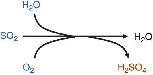
CO2–H2O–SO2
H2O + SO2 only does not have a significant influence on the formation of a separate acid phase, due to the necessity of high reactant concentration limits for acid formation and dropout, and also potentially low reaction kinetics.
CO2–H2O–SO2–O2
O2 oxidizes SO2 to SO3 and its reaction with water causing the formation of H2SO4. Reaction has been experimentally observed, but requires high reactant concentrations and is potentially associated with low kinetics.
Note 2—H2SO4 has a low solubility in dense CO2 (much lower than HNO3), and once formed dropout can take place [32].
CO2–H2O–SO2–O2–H2S
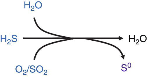
Elemental sulfur might form and drop out. Kinetics of reaction is however low and alternative reactions may take place first. This reaction has been observed where sufficient H2S is present.
CO2–H2O–SO2–NO2
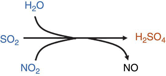
The additional presence of NO2 plays a strong catalytic role in the formation of H2SO4: The reaction H2O + SO2 + NO2 leads to the formation and dropout of H2SO4 at much lower concentrations of SO2 (compared to H2O + SO2 or H2O + SO2 + O2).
See Note 2.
CO2–H2O–SO2–NO2–H2S
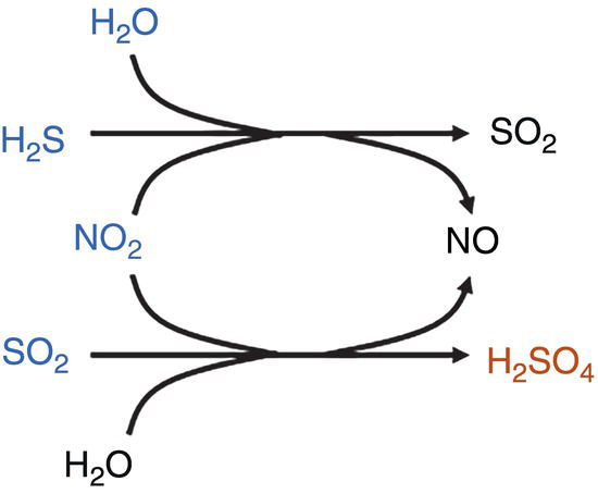
H2S and NO2 are expected to react first to form SO2 + NO. Then, H2O, NO2, SO2 can react to form H2SO4.
The combination of H2S and NO2 seems to trigger a much lower SO2 limit for the formation and dropout of H2SO4, and act as an initiator for other reactions at relatively low concentrations.
See Note 2.
CO2–H2O–SO2–NO2–H2S–O2
H2O and H2S react with NO2 to form NO and SO2. The presence of O2 can react with the NO to react and form NO2 again, making it available to stimulate the formation of H2SO4 or react to produce HNO3. Formation of S can be expected, if there is an excess of O2 and H2S
See Notes 1 and 2.
CO2 Pressure (bar)
Temperature (°C)
Water Content (ppm mole)
Exposure Time (hours)
Uniform Corrosion Rate (mm/year)
Author and Reference
95–182
50–130
Water-saturated CO2
96
0.014–0.043
Zhang et al. [34]
123–146
25–60
Water-saturated CO2
48–400
0.01–0.1
Cabrini et al. [35]
100
20–25
1220
720
None (stagnant) and <0.01 (flow)
Dugstad et al. [36]
100
8–25
100–2500
720
<0.001 (flow)
Morland et al. [37]
80
50
Water-saturated CO2 (~3400 ppm)
24
~0.4
Choi et al. [38]
80
50
Water-saturated CO2 (~3400 ppm)
48
~0.024
Hua et al. [39]
2650
0.014
1600
None reported
700
None reported
80
40
3660
168
0.08
Sim et al. [40]
1220
0.08
976
0.08
732
0.06
488
0.07
244
0.08
80
35
Water-saturated CO2 (~3437 ppm)
48
~0.1
Hua et al. [39]
2800
0.068
1770
0.028
1200
0.012
700
0.005
300
0.004
CO2 Pressure (bar)
Temperature (°C)
Water Content (ppm mole)
Exposure Time (hours)
Pitting Corrosion Rate (mm/year)
Author and Reference
80
50
Water-saturated CO2 (~3400 ppm)
48
1.99
Hua et al. [39]
2650
0.20
1600
None reported
700
None reported
80
40
Water-saturated CO2
168
0.19 (average)
0.50 (max)
Sim et al. [40]
3500
0.22 (average)
0.65 (max)
2600
0.22 (average)
0.55 (max)
1800
0.3 (average)
0.64 (max)
900
0.22 (average)
0.65 (max)
80
35
Water-saturated CO2 (~3437 ppm)
48
0.92
Hua et al. [39]
2800
0.85
1770
0.62
700
0.29
300
0 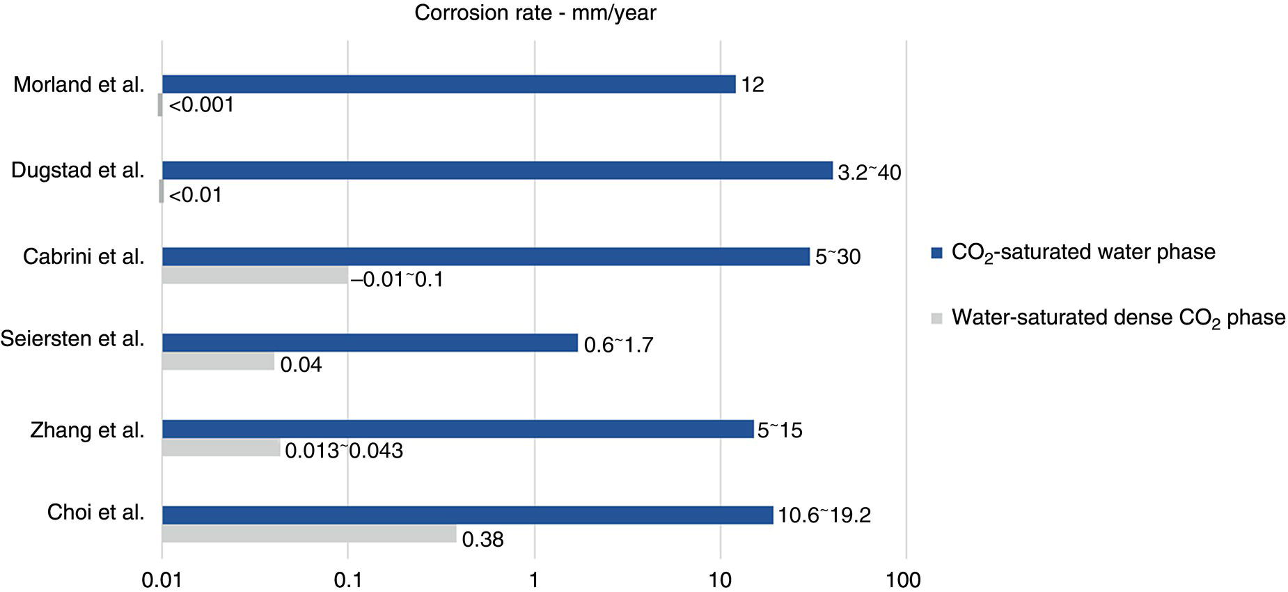
CO2 Pressure (bar)
Temperature (°C)
Exposure Time (Days)
Flow
Corrosion rate mm/year
References
150
50
1–3
3 m/s
41.7
[37, 44]
120
65
2
Stat
16.4
[45]
120
90
2
Stat
7.3
[45]
100
10
14
Stat
0.5
[46]
100
12
1–3
1 m/s
6.3
[37, 46]
100
13
1–3
1 m/s
3.2
[37, 46]
100
13
1–3
3 m/s
6.2
[37, 46]
100
25
5
0.65 m/s
12
[47]
100
50
14
Stat
2.7
[46]
100
50
1–3
1 m/s
33
[37, 46]
100
50
1–3
3 m/s
38.3
[37, 46]
95
40
6–12.5
<<1 m/s
0.6
[48]
95
50
4
Rotating cage
5.9
[49]
95
50
4
Rotating cage
8.9
[50]
95
50
7
Stat
5
[51]
95
80
7
Stat
7
[51]
95
80
Inst.
Stat
17.2
[51]
95
110
7
Stat
2
[51]
95
130
7
Stat
1.9
[51]
87
25
0.65 m/s
11.5
[52]
85
40
6–12.5
<<1 m/s
1.7
[48]
80
50
1
Stat
19
[45]
80
50
5–7
Stat
4.6 (av)
[51]
80
65
2
Stat
12.8
[45]
80
90
2
Stat
5.6
[45]
75
25
0.65 m/s
11.6
[52]
60
50
1
Stat
20
[53]
58
40
6–12.5
<<1 m/s
4.4
[48]
50
25
0.65 m/s
11.5
[52]
40
25
0.65 m/s
10.9
[52]
40
50
1
Stat
18
[53]
40
65
2
Stat
11.1
[39]
40
40
6–12.5
<<1 m/s
4.9
[48]
40
50
5–7
Stat
6.9 (av)
[54]
40
90
2
Stat
5.5
[45]
20
50
5–7
Stat
4.3 (av)
[54]
10
25
0.65 m/s
10.2
[52]
10
40
6–12.5
<<1 m/s
5.6
[48]
10
50
7
Stat
1.2
[51]
10
80
7
Stat
1.8
[51]
10
80
Inst.
Stat
28.3
[51]
10
110
7
Stat
1.1
[51]
10
130
7
Stat
1
[51] 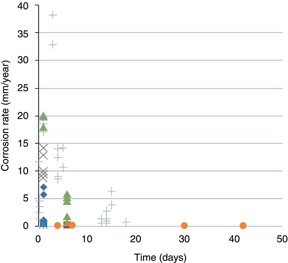
Pressure (bar)
Temperature (°C)
H2O (ppmv)
SO2 (ppmv)
Exposure (days)
CR (mm/year)
Reference
100
25
488
500
14
0.01
[37]
100
25
488
344
14
<0.005 (spot)
[25]
100
25
1220
344
14
0.02 (spot)
[25]
100
25
1220
500
14
0.02
[15]
100
50
Saturated
1000
5
0.47
[46]
80
50
650
1%
1
3.48
[52]
80
50
650
0.10%
1
0.03
[50]
80
50
650
0.05%
1
0.05
[56]
80
50
650
0.10%
1
6.8 (pitting)
[53]
80
50
3310 (sat)
1%
1
5.6
[57]
75.8
40
2440
100
4.6a
[54]
Pressure (bar)
Temperature (°C)
H2O (ppmv)
NO2 (ppmv)
Exposure (days)
CR (mm/year)
Reference
100
25
488
500
10
1.6
[15]
100
25
488
96
3
0.15
[37]
100
25
488
191
20
~0.05
[37]
100
25
1220
200
10
0.67
[15]
100
50
500
50
1
0.127
[58]
100
50
500
100
7
0.02
[59]
100
50
500
200
1
0.205
[59]
100
50
500
200
3
0.088
[59]
100
50
500
200
7
0.025
[59]
100
50
500
200 (NO)
7
0.013
[59]
99
26
670
70
–
0.84
[32]
75.8
40
2440
100
Instantaneous
11.6a
[60]
Pressure (bar)
Temperature (°C)
H2O (ppmv)
H2S (ppmv)
Exposure (days)
CR (mm/year)
Reference
140
3
1000
800
28
<0.0005
[61]
140
22
1000
800
42
<0.0005
[62]
120
80
Saturated
200
2
0.41
[63]
80
80
100
200
1
<0.01
[64]
Pressure (bar)
Temperature (°C)
H2O (ppmv)
O2 (ppmv)
Exposure (days)
CR (mm/year)
Reference
100
50
Saturated
200
5
0.6 (pit: 17)
[46]
100
50
500
500
7
0.006
[59]
100
50
Saturated
1000
5
0.03
[63]
80
50
Saturated
4%
1
~1
[57]
80
50
3000
4%
1
<0.01
[57]
80
50
650
4%
1
<0.01
[57]
80
35
Saturated
20
2
0.09
[40]
80
35
Saturated
500
2
0.07
[40]
80
35
Saturated
1000
2
0.03
[40]
80
35
300
1000
2
0
[40]
80
35
650
1000
2
0
[40]
80
35
1200
1000
2
0.002
[40]
80
35
1770
1000
2
0.005
[40]
80
35
2800
1000
2
0.012
[40]
75.8
40
2440
100 ppmw
Instantaneous
2.3a
[60]
Pressure (bar)
Temperature (°C)
H2O (ppmv)
SO2 (ppmv)
O2 (ppmv)
Exposure (days)
CR (mm/year)
References
100
20
488
1000
100 ppmw
7
0.01
[15, 37]
100
20
488
200
100 ppmw
7
<0.01
[15, 37]
100
25
488
1000
100
7
0.01
[25, 57]
100
25
488
200
100
7
<0.01
[25, 65]
100
50
Saturated
1.40%
0.10%
12
~0.8
[56, 60, 66]
100
50
Saturated
0.20%
0.10%
12
0.15
[67–69]
100
50
Saturated
2.00%
0.10%
5
~0.9
[67–69]
100
50
50%RH
2.00%
0.10%
5
0.04
[67–69]
100
50
Saturated
1000
1000
5
1.034
[63]
99
26
1900
80
220
0.009
[32]
80
50
0
1%
4%
1
No attack
[57]
80
50
650
1%
4%
1
3.7
[57]
80
50
3310 (sat)
1%
4%
1
7
[57]
80
35
3437 (sat)
50
20
2
G:~0.35 P: ~1.7
[28]
80
35
3438 (sat)
100
20
2
G:~0.7
P:~1.7
[28]
80
35
1770
50
20
2
G:~0.025–0.03
P:~1.1
[28]
80
35
1770
100
20
2
G:~0.06
P:~1.5
[28]
80
35
700
50
20
2
G:~0.006
P:~0.23
[28]
80
35
700
100
20
2
G:~0.004
P:~0.018
[28]
80
35
300
50
20
2
~0.003
[28]
80
35
300
100
20
2
~0.003
[28]
Pressure (bar)
Temperature (°C)
H2O (ppmv)
NO2 (ppmv)
O2 (ppmv)
Exposure (days)
CR (mm/year)
Reference
100
50
500
50
500
1
0.116
[59]
100
50
500
100
500
1
0.182
[59]
100
50
500
200
500
1
0.275
[59]
100
50
500
200
500
7
0.09
[59]
100
50
500
200 (NO)
500
7
0.03
[59]
100
50
50
100
500
7
0.05
[59]
100
50
50
100
10000
7
None reported
[59]
Pressure (bar)
Temperature (°C)
H2O (ppmv)
SO2 (ppmv)
NO2 (ppmv)
Exposure (days)
CR (mm/year)
References
100
25
488
138
191
7
0.017
[25, 65]
Pressure (bar)
Temperature (°C)
H2O (ppmv)
SO2 (ppmv)
NO2 (ppmv)
H2S (ppmv)
O2 (ppmv)
CO (ppmv)
Exposure (days)
CR (mm/year)
Reference
110
60
1000
70
100 (NO)
4.70%
50
7
0.015–0.073
[59]
110
60
1000
70
100
8100
750
7
0.03
[62]
110
60
1000
70
100
8100
750
7
0.025
[64]
110
60
1000
70
100
8100
750
7
0.003
[65]
100
25
122
69
96
130
275
10
0.034
[67]
100
25
300
100
100
100
350
6
0.04
[68]
100
45
300
100
100
100
350
6
0.05
[70]
100
50
Saturated
1000
1000
1000
5
1.4
[63]
99
25
90
30
32
36
70
–
0.1
[32]
5.4.1.3 Environmentally Assisted Cracking (Internal)
CO2–CO–H2O
H2S and Sour Cracking
H2, Hydrogen Embrittlement and Fatigue
5.4.2 Fracture Control9, [79]
5.4.2.1 Why Is It Needed?
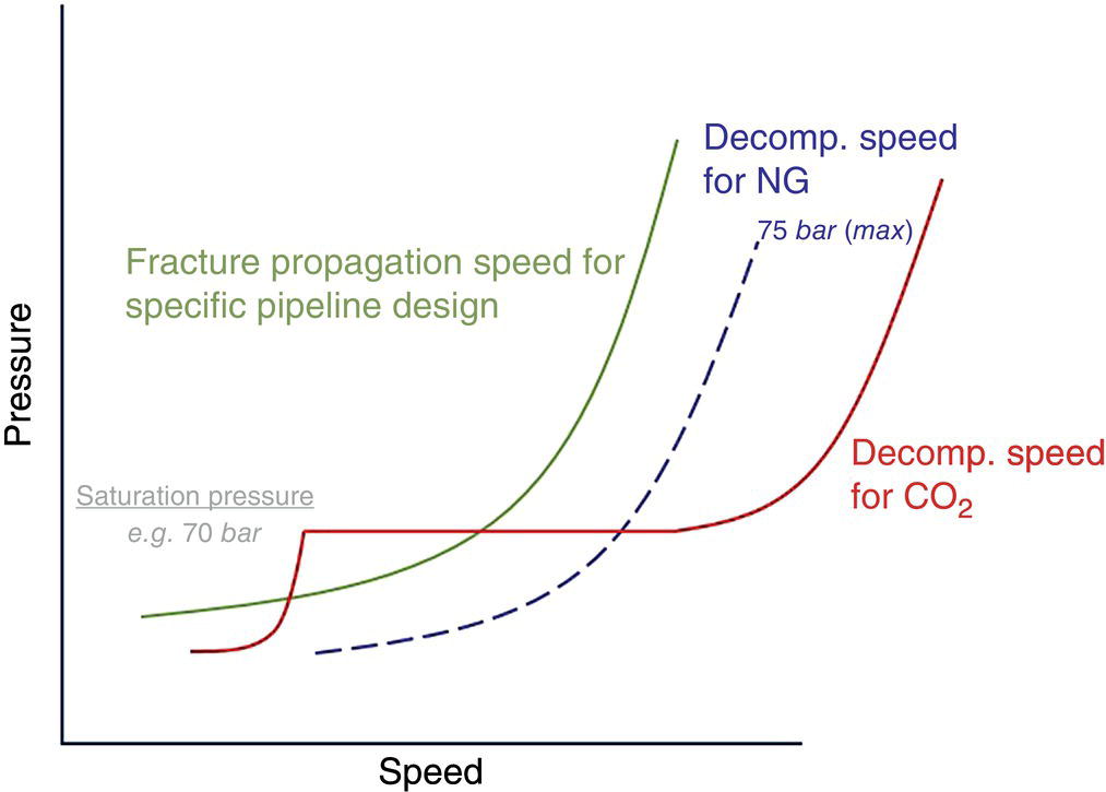
5.4.2.2 Toughness Requirements and Challenges
Requirement
Pipe Body
Weld
Individual (J)
Average (J)
Individual (J)
Average (J)
BS EN ISO 3183/API 5L PSL2a
20
27
20
27
BS EN ISO 3183/API 5L Annex Gb
34
46
No explicit additional requirements for welds
Project-specific CO2 installation piping (gaseous and dense phase)
30
40
41
47
Project-specific line pipe CO2 (gaseous phase)
38
48
41
47
Project-specific line pipe CO2 (dense phase)
188
250
41
47
5.4.2.3 The Impact of Impurities on the Fracture Toughness Criterion
5.4.3 Integrity Experience of Existing CO2 Pipelines and Cautions
5.4.3.1 A Positive Experience?
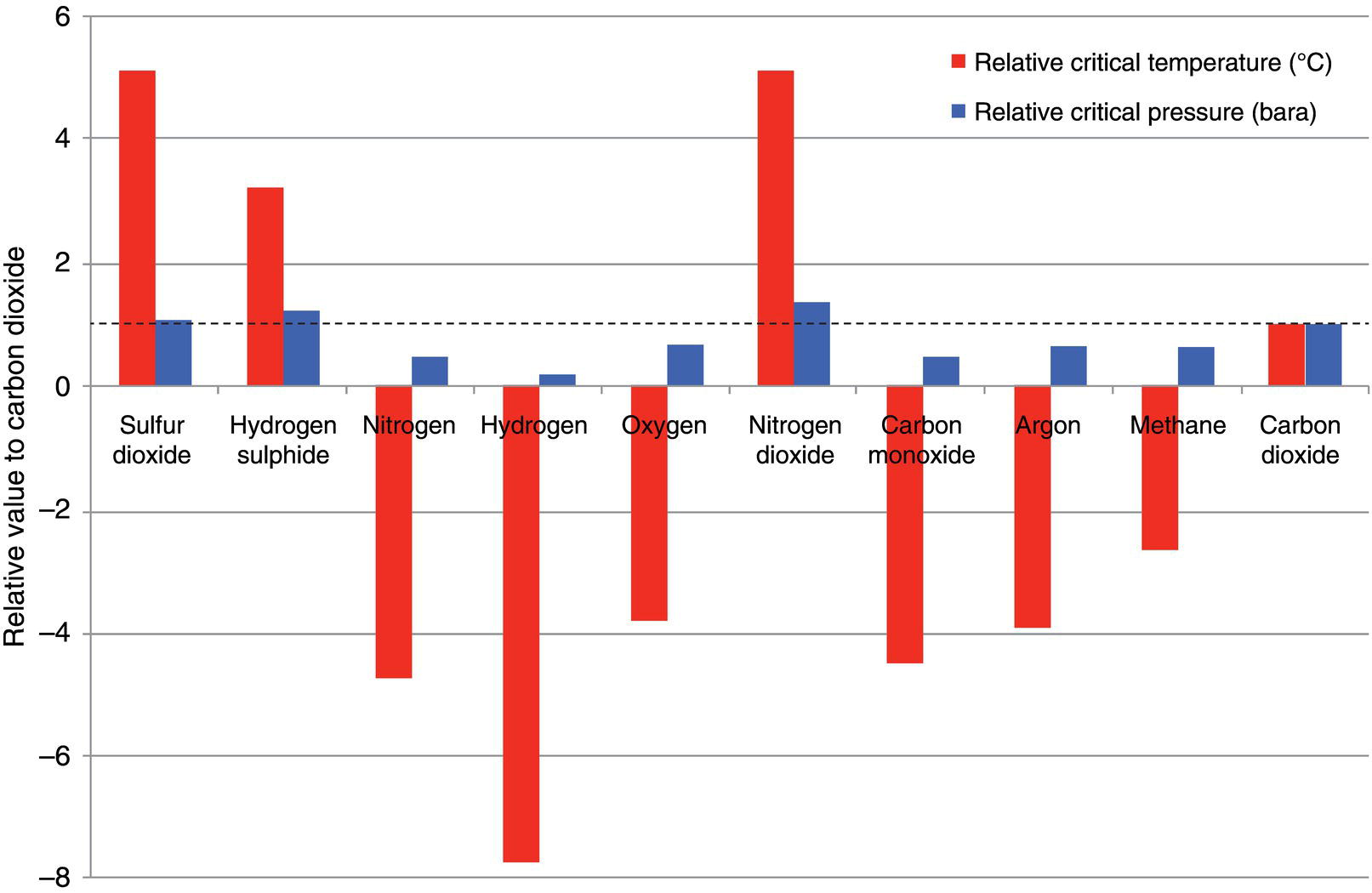
5.4.3.2 Cautions
5.5 Managing the Safe Repurposing of Vintage Pipelines
5.5.1 Defining CO2 Stream Specifications
Impurity
Impact on Pipeline Integrity
Sonke and Zheng [31] Proposed Limits for Carbon Steels (ppm mole)
ARAMIS Project Proposed Specification Limits for Pipelines
Internal Corrosion
Internal SCC
H 2 O
Risk of aqueous phase formation and dropout
100 ppm (risk of acid dropout validated for 100 bar at 25 °C)
Note: can be relaxed in the absence of SO2, NO2, O2, H2S
<70 ppm mole
NOx (NO 2 + NO)
Highly reactive; results in the formation of a free water phase containing strong acids HNO3 and H2SO4 at water concentrations much lower than solubility limits
Catalyst for other reactions, including formation of H2SO4
Most aggressive impurity on the corrosion rate of carbon steel (e.g., more aggressive than SO2 at low water contents)
Lowers pH and destabilization of protective corrosion product films (e.g., film formed during the nitric acid–induced corrosion of carbon steel is dusty without protective properties)
Note 1: H2SO4 has a low solubility in dense CO2, and once formed, dropout can take place. In contrast, HNO3 has a high solubility in dense CO2 [32]
Low pH—increase sour crack threat in presence of H2S?
Note—NO2 reacts with H2S to form SO2; this reaction can effectively lower the content of H2S in the water phase and thus reduces sour crack threat. However, to take credit for this effect, the presence of a minimum NO2 concentration must be ensured, which is not practical and safe
2.5 ppm (risk acid dropout validated for 100 bar 4 °C)
Note: Other limits may be relaxed in the absence of NO2
<2.5 ppm mole
SOx (SO 2 + SO3)
Lowers tolerable water content due to the formation of acids H2SO3 and (in presence of O2) H2SO4
Acid formation may be, however, associated with low kinetics, but it is significantly enhanced in the presence of NO2
Low pH—increase sour crack threat in presence of H2S?
10 ppm (risk of acid dropout validated for 100 bar 25 °C)*
–
H 2 S
Can produce elemental sulfur in the presence of O2. Kinetics of reaction is, however, low, and alternative reactions may take place first. This reaction has been observed where sufficient H2S is present
Elemental sulfur has the potential to accumulate within the system and negatively impact the permeability of formations by clogging pore systems. It leads to corrosion in the presence of water
Forms SO2 in the presence of NO2 (and then H2SO3 and/or H2SO4)
Can induce sour cracking but limits not yet defined (ongoing research)
10 ppm (risk of acid dropout validated for 100 bar 25 °C)*
<5 ppm mole
H 2 S + SO x
–
–
20 ppm (risk of acid dropout validated for 100 bar 25 °C)*
Note: Limit to include carbonyl sulfide (COS) if present
Note: Limit may be relaxed in the absence of NO2. 60 ppm has been identified as a safe limit
H2S + COS + SOx + DMS <20 ppm mole
O 2
Leads to the formation of strong acids and elemental sulfur
Accelerates corrosion rates
Naturally shifts the electrochemical potential in the region susceptible to SCC; increases susceptibility to CO2–CO–H2O SCC
20 ppm (risk of acid dropout validated for 100 bar 25 °C)*
<40 ppm mole
CO
–
Threat of CO2–CO–H2O SCC
At 20 °C 50 bar CO2 with and without methanol 1000 ppm CO did not initiate cracking [71]
1000 ppm
Note: Validation did not include a full range of impurities, only the effect on the water dew point was considered
<75
H 2
–
Hydrogen embrittlement and fatigue growth to be considered
No significant impact was observed at 2 bar H2 equivalent to 1% H2 at 200 bar CO2 [72]
No significant impact was observed at 2 bar H2 equivalent to 1% H2 at 200 bar CO2
<7500 mole
Glycol (MEG, TEG, DEG)
Impurity from the dehydration process. Hygroscopic component. Leads to the formation of separate aqueous phase and drop out below water solubility limits. This induces CO2 corrosion but rates are inhibited depending in glycol concentration in water phase. Research ongoing to characterize applicable corrosion rates
Increase of pH can inhibit sour cracking
MEG ~5 ppm
TEG <1 ppm
Note: Validation did not include a full range of impurities, only the effect on the water dew point was considered
Follow dew point specification (dew point of any liquid phases less than −10 °C @20 bar)
Methanol, ethanol
Hygroscopic component. Presence of alcohol influences water phase drop out below dew point. Leads to the formation of separate aqueous phase and drop out below water solubility limits. This induces CO2 corrosion but rates are inhibited depending in glycol concentration in water phase. Research ongoing to characterize applicable corrosion rates
Increase of pH can inhibit sour cracking
Unknown
Methanol <620 ppm mole
Ethanol <20 ppm mole
Amines (e.g., MDEA)
Hygroscopic component. Presence may influence water phase drop out below dew point. May lead to the formation of separate aqueous phase and drop out below water solubility limits. This induces CO2 corrosion but rates are inhibited depending of amine concentration in water phase. Research to be conducted
Increase of pH can inhibit sour cracking
Unknown
<1 ppm mole
HCl
Strong acid and will acidize any water present
Low pH—increase sour crack threat in presence of H2S?
Unknown
–
HCN
Weak acid promotes acidification and destabilizes protective films
Low pH and promote H adsorption—increase sour crack threat in presence of H2S?
Unknown
<2 ppm mole
Organic acids
Promote acidification and destabilize protective films
Low pH—increase sour crack threat in presence of H2S?
Unknown
–
N 2
Inert—no negative impact expected
–
Inert
<2.4 mole%
Ar
Not expected to be a significant influence
–
Unknown
<0.4 mole%
Aldehydes
May influence water solubility
–
Unknown
Total <10 ppm mole
Phosphorous components
May be reactive. No data available
–
Unknown
Total <1 ppm mole
Aromatics
May have some effect in line with phenolics, not yet investigated
–
Unknown
Total <0.1 ppm mole
5.5.2 Understanding Line Pipe Material Properties for Fracture Control
5.5.3 Defining Integrity Baseline Condition and Confirming MAOP
Challenges
Affected Components
Reasons
Chemical degradation and explosive decompression
Nonmetallic—multiple; e.g., cables, sensors, seals
Interaction with dense CO2; explosive decompression (end of ILI run)
High wear
Tool cup and disks
Dry environments
Damage of electronic components
Electronic components
Build-up of electrostatic charge on tool due to movement of cups along pipe wall in dry environment
Leads to high voltages between tool and pipeline, resulting in discharge, which might lead to damage on tool or on pipeline
Depends on position and intensity of discharge
5.5.4 Managing Safe Operations: Inspections
References
Notes