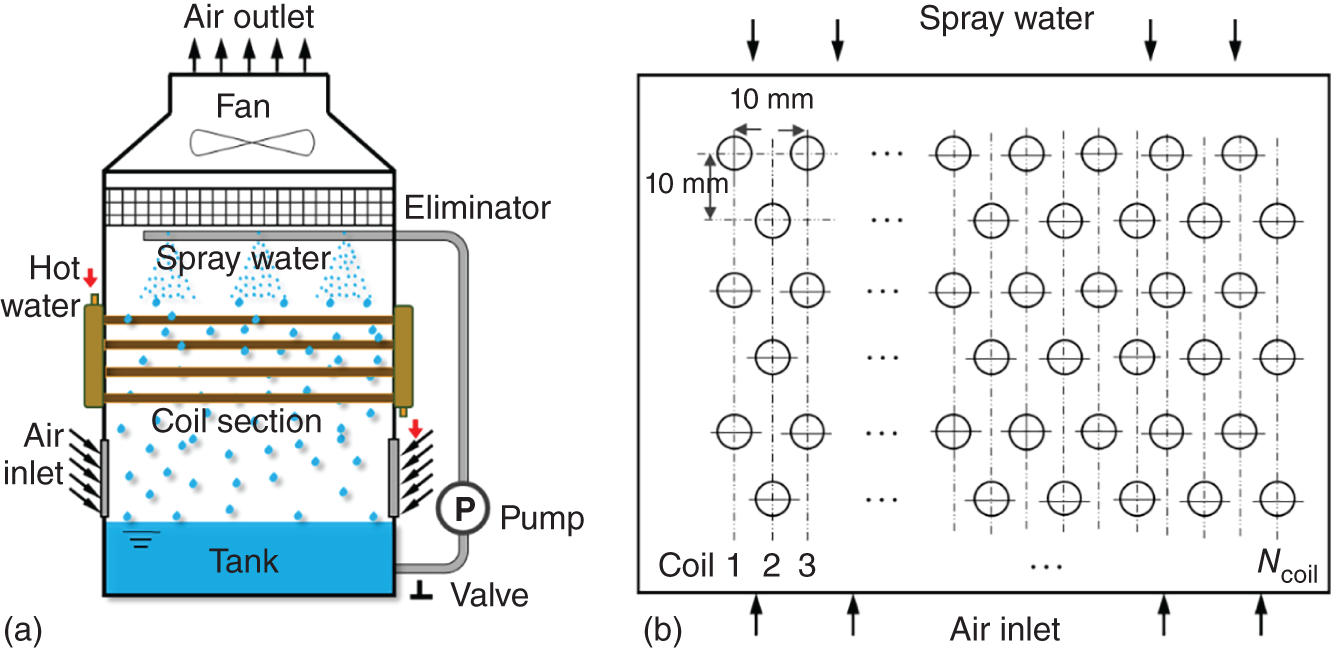
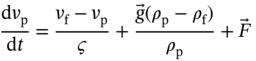
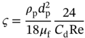
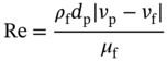
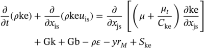
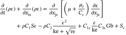
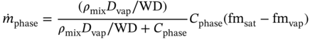
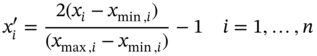
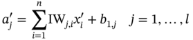
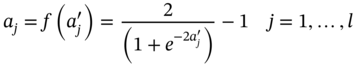
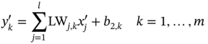
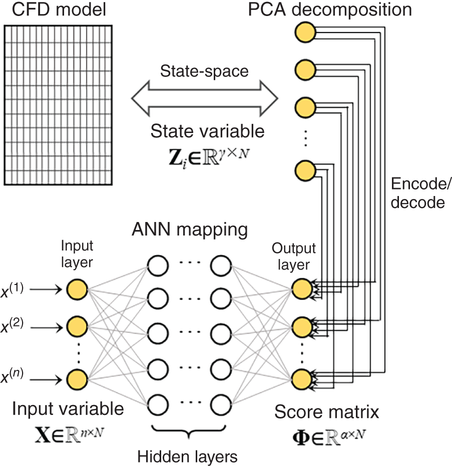
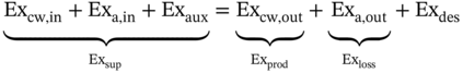
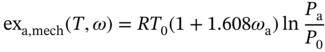
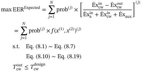
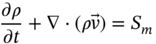
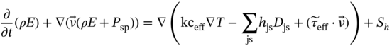
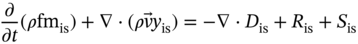
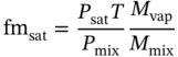
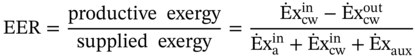
1Sun Yat-Sen University, School of Chemical Engineering and Technology, No. 135, Xingang Xi Road, Zhuhai, Guangdong, 519082, China 2The Key Laboratory of Low-carbon Chemistry & Energy Conservation of Guangdong Province, Guangdong Engineering Center for Petrochemical Energy Conservation, 132 Waihuan East Road, University City, Panyu District, Guangzhou, 510275, China 3Sun Yat-Sen University, School of Materials Science and Engineering, Guangzhou, No. 135, Xingang Xi Road, 510275, China The process industry has long relied on cooling towers to enhance sustainability by removing waste heat from circulating water, particularly in the face of increasing water scarcity [1, 2]. However, in certain regions, traditional open cooling towers struggle to effectively cool circulating water or experience high evaporative losses due to significant seasonal fluctuations. In response to these challenges, more sophisticated closed-type cooling systems, such as closed-wet cooling towers [3, 4] and hybrid closed-circuit cooling towers [5, 6], have been recently developed to address these issues and are particularly well-suited for heat rejection and water conservation in diverse weather conditions. To ensure their flexible operation, it is crucial to thoroughly understand the interplay between operating conditions, weather conditions, and the thermodynamic performance of these cooling tower systems. For instance, in hot and humid weather, cooling towers may not operate at their optimal level, necessitating measures to enhance their efficiency. During cold and dry weather, conversely, they may perform excessively, requiring conservative measures to prevent over-cooling. This entails a need not only to develop accurate prediction models but also to utilize these models for optimal design and management. Closed-type cooling tower models often involve complex interactions between fluid dynamics and heat-mass transfer processes as well as various contacting patterns of vapor–liquid outside the coil tubes [7, 8]. With the advancement of computational fluid dynamics (CFD), numerical studies have become the primary approach to gaining a deeper understanding of these processes through a detailed full-order model (FOM). The FOM can provide an accurate spatially distributed parameter description of the coupled heat and mass transfer processes by considering the detailed multiphase interactions, transport effects, and phenomena at a broader length scale. For example, the profiles of temperature and humidity of the inlet air in the air–liquid contact units of the cooling towers are unevenly distributed and varied with uncertain and control parameters, which define the spatial heterogeneities of the humid and thermal characteristics of the air in the flow field. Deciphering such distributed parameters in detail is conducive to improving the overall thermodynamic performance of the cooling towers. In theory, the solution of the FOMs of cooling tower systems involves tracking the multiphase interactions and the spatial movement of each liquid droplet, characterized by computationally expensive partial differential equations (PDEs). It is noted that the benefits of constructing FOMs must be balanced against the computational resources and time required to develop them, which can be a major obstacle to improving cooling systems [3]. For example, a single task of the 3D CFD model of a closed-wet cooling tower system normally takes more than 30 CPU hours by using the Reynolds averaged Navier–Stokes turbulence model [7, 9]. The computational burden would significantly limit the use of the principled CFD simulation for real-time prediction and multivariable analysis. It becomes more critical as the FOM is embedded in an equation-oriented optimization task because a large size of recourses to the CFD models have to be executed before converging to the optimum. The reduced-order model (ROM) of a CFD-based model is a surrogate model for input-to-output mapping due to the computationally expensive nature of high-fidelity simulation, which entails iterative calculations. Surrogate-based model reduction is one of the practical solutions to construct a more tractable model as an alternative to computationally expensive FOM without loss of fidelity by only approximating the input–output relationship of a system [10]. Given input parameters (i.e. initial, boundary, and operational conditions), the quantities of interest for calculating distributed parameters at each mesh point, such as velocity, pressure, temperature, and moisture content, can be obtained rapidly without conducting principled CFD simulation. The model reduction approach can be roughly categorized into two categories: physics-based models and data-driven models [11, 12]. In the former, a reduced basis is extracted from the simulation data using an unsupervised learning technique, e.g. principal component analysis (PCA), in which the FOM operator is projected onto the subspace spanned by the reduced basis [13]. As a result, the degrees of freedom of the original system can be significantly reduced by retaining the underlying basic structure of the FOM. Another way to enable rapid simulations is to build a data-driven model, where a response surface of the system is learned from the simulation data in a supervised manner. The deterministic or probabilistic mapping models of input–output can be constructed using, e.g. polynomial basis functions [14], radial basis functions [15], Gaussian process [16], and stochastic polynomial chaos expansion [17]. The objective of this chapter is to create an integrated optimization approach using bi-level model reduction to efficiently determine the optimal thermodynamic performances and their corresponding spatially distributed parameters. This approach involves combining a data-driven ROM and a physics-based ROM, achieved through a series of statistical methods including optimal experiment design, multi-sample CFD simulation, bi-level model reduction, and model evaluation. The design of experiments (DoE) aims to maximize the process information obtained from a finite number of CFD simulations by carefully selecting experimental points. Subsequently, two types of surrogate models can be developed using model order reduction and data-driven techniques, enabling their substitution for the original FOM in design and optimization tasks using efficient nonlinear programming techniques. This chapter is derived from the work of He and coworkers [4, 9, 18, 19]. The physical model of cooling towers investigated in this study is based on a bench-scale closed-wet cooling tower experimental set-up [8] with parallel counter-flow construction. As shown in Figure. 8.1a, the ambient air flows upward and traverses the outer wall of the tube bundle using the intake fan in countercurrent flow with the spray water. The tube bundle’s cross section shown in Figure 8.1b is arranged in a triangular pattern, with adjacent tubes in each row having the same centerline spacing. The hot circulating water pumped from the main tube is evenly divided and distributed across the serpentine tubes inside the tower casing, where its sensible heat is indirectly absorbed by film evaporation and upward air flow outside the tube bundle. The heat and mass transfer processes of water film are mainly sustained by the joint effect of countercurrent spray water and ambient air. A small proportion of spray water diffuses together with the upward airflow due to evaporation, and the remaining portion leaving the water film is collected in a water tank and finally returns to the top nozzles through the spray water pump. Therefore, the circulating water relies on the film evaporation to achieve the required cooling targets, such as temperature drop and heat dissipation. Figure 8.1 (a) Sketch of the cooling tower set-up and (b) cross section of the tube bundle [4, 9]. In the investigated cooling tower, the complex heat and mass transfer processes outside the tubes can be mathematically described by large-scale PDAEs that are constructed from mass and energy conservation and hydrodynamic equations. These equations can be written in general transport equation form, as presented in Eqs. (8.1)–(8.14). Among them, the Navier–Stokes and energy conservation equations are as follows: where Sm is the mass added to the continuous phase from the dispersed second phase; Psp and To numerically simulate the dynamics of multiphase flows, we use the Eulerian–Lagrangian approach, as described in previous studies [20–22]. In this approach, the air-fluid phase is treated as a continuous medium, and its behavior is modeled by solving the Navier–Stokes equations. On the other hand, the dispersed phase, represented by the spray water, is treated as a collection of particles or droplets. The motion of these particles or droplets is tracked by integrating the force balance equation, allowing for the exchange of momentum, mass, and energy with the fluid phase. The force balance equation is formulated to equate the particle’s inertia with the forces acting upon it. Mathematically, this can be expressed as follows: where vf, μf, and ρf are the velocity, molecular viscosity, and density of the fluid, respectively; vp, ρp, and dp are the velocity, density, and diameter of the particle, respectively; (vf − vp)/ζ is the drag force per unit particle mass; and Re is the relative Reynolds number. According to previous studies [8, 23], the realizable k–ε model that presents a sufficient adaptation with the physics of flow turbulence is applied to model the turbulent flow outside the tubes in the tower. Based on the general form of the transport equation, the turbulence kinetic energy ke, and its rate of dissipation ε, are obtained from the realizable k–ε model equations, which are expressed as follows: where Gk and Gb represent the generation of turbulent kinetic energy due to the mean velocity gradients and buoyancy; yrM is the contribution of the fluctuating dilatation in compressible turbulence to the overall dissipation rate; C2 and C1ε are constants; and Cke and Cε are the turbulent Prandtl numbers for parameters ke and ε. The mixture special transport model is employed to calculate the concentration of different species in the cooling tower, and the convection-diffusion equation is used to solve these given by Eq. (8.9). where fmis, Ris, Dm,is, and DT,is are the mass fraction, net rate, mass diffusion, and thermal diffusion coefficients for species is, respectively; Sct is the turbulent Schmidt number; and the default is 0.7. The Eulerian wall film model, coupled with the mixture species transport model, is used to calculate phase changes between film liquid and gas vapor. The rate of phase change is governed by: where ρmix is the density of the gas mixture; Dvap is the mass diffusivity of the vapor species; WD is the cell-center-to-wall distance; Cphase is the phase change constant; fmvap is the mass fraction of the vapor species. In addition, fmsat and Psat calculated via Eqs. (8.12) and (8.13) are the mass fractions and pressure of saturation species, Mvap and Mmix are the molecular weights of the vapor species and mixture, and Pmix is the absolute pressure of the gas mixture. The droplet temperature is updated according to the energy balance shown in Eq. (8.14) that relates the sensible heat change between the droplet to the convective and latent heat transfer between the droplet and the continuous phase: where cpp is the droplet heat capacity, ht is the convective heat transfer coefficient, T∞ and Tp are the temperatures of the continuous phase and droplet, dmp/dt and Qlh are the evaporation rate and latent heat, and CSB is the Stefan–Boltzmann constant. In the context of model reduction for specific process equipment, three types of variable spaces are considered: the input space X, the output space Y, and the state space Z in the fluid field. Figure 8.2 illustrates the interconnection of matrices representing these three variable spaces, which is crucial for constructing the bi-level ROMs. In the cooling tower system depicted, there are n inputs and m outputs, while s state variables are monitored across a total of γ discretized elements. The steady-state nonlinear relations between the state and output variables, corresponding to the input variables, can be described by the following state-space model [13]: where B and D are the mapping coefficient matrices and x, y, and z are the input, output, and state vectors, respectively, which contain the variables related to calculating the objective function and physical field. The input, output, and state spaces for the CFD model of cooling towers should be defined before the experimental design. The input vector x in the input space is provided in Table 8.1. For a given inlet boundary condition, it contains the values of all variables in the input streams entering the cooling tower system, i.e. uncertain variable x(1) = [ Figure 8.2 The construction of bi-level ROMs. Table 8.1 Input space for the model parameters. For constructing the bi-level ROMs of cooling towers with high fidelity, it is necessary to build the mappings between the aforementioned input and output vectors, as well as between the input and state vectors. For this purpose, much effort is required to collect and handle a huge amount of data obtained from a batch of principled CFD simulations of the equipment item. The main steps are summarized as follows: Evaluate the generalization performance of the developed bi-level ROMs. More details about these four steps are provided in the following Sections 8.3.1–8.3.3. Batch simulations of principled CFD models are often computationally intensive and time-consuming, necessitating the reduction of computational resources. DoE is a suitable approach for maximizing the amount of process information obtained from a fixed number of observations by selecting appropriate design points. Various methods can be used to implement DoE, such as Monte Carlo sampling, Taguchi experiments, probabilistic collocation, and stochastic collocation. Herein, a low-dimensional discrete approximation method called the stochastic reduced-order model (SROM) is utilized to generate a finite set of stochastic samples with varying probabilities. The SROM method can be considered a “smart” Monte Carlo method for uncertainty quantification, as it can efficiently discretize the input space and reduce the computational complexity associated with propagated uncertainty, while maintaining the nonintrusive nature of the method [18]. A detailed description of the SROM method is provided below. Let us consider the probabilistic behavior of X = An SROM Similar to X, the statistics of the SROM where I(A) is a binary function, I(A) = 1 if A is true, otherwise I(A) = 0. The discrepancy between The optimal SROM where the coefficients To obtain the mapping data for constructing the ROMs, the uncertainty associated with the input variables is propagated by executing the rigorous CFD simulation of the cooling tower model for each of the SROM samples. The multi-sample CFD simulation is performed on the meshed geometry of the cooling tower system to calculate the coupled heat and mass transfer processes, as well as the mass and energy balances of the PDEs. Note that the circulating water inside the tubes relies on film evaporation to achieve the required cooling targets, such as temperature drop and heat dissipation. Thus, we only focus on the heat and mass transfer processes of the water film outside the tube bundle at the coil section, which is stimulated by a 3D CFD model of flow, temperature, and pressure fields. The following assumptions are made to reduce the complexity of the cooling tower model: The process geometry of the coil section shown in Figure 8.1b is constructed based on the standard diameter and length in the COMSOL modeling environment. It consists of 19 rows and 12 columns of bare-type copper tubes in the 0.61 × 1.2 × 0.68 m3 domain. The preliminary sketch is meshed to adequately capture the change of fluids by using the meshing module. To enhance model accuracy and reduce computational load, it is necessary to fine-tune the mesh system near the tube walls before running the numerical program. As shown in Figure 8.3, a five-layer boundary layer grid scheme is implemented with a stretching factor of 1.2 for the inner and outer walls of the tube. This choice aims to improve the accuracy and stability of predictions. Tetrahedral meshes are employed for the remaining space. Moreover, the element size is gradually stretched to effectively capture high-gradient regions, ensuring a proper resolution of temperature and velocity fields. Thus, the computational domain is extended by 0.09, 1.2, and 0.68 m in x-, y-, and z-axes, respectively. The mesh structure has 1 114 893 nodes, and only 3 304 nodes are presented in the cross section along the center of the coil tube. The quality of this mesh structure, measured by the skewness value, should be satisfied at the required level. In each CFD model, the RNG k–ε turbulence modeling approach is applied to simulate the mean flow characteristics of the air and water in turbulent flow conditions. The governing equations with boundaries are solved by the finite element method, and a segregated solver sequence was selected to handle the highly nonlinear models. Moreover, the source terms of moisture transport and heat transfer [4, 18] are added to the governing equations for accurately describing the heat and mass transfer processes. Figure 8.3 The mesh structure of the computational domain generated by COMSOL@ at (a) entirety, (b) lateral section, (c) mesh along the air outlet, (d) mesh along the tube walls, and (e) mesh near the tube walls [9, 18]. Color represents the value of skewness. The data-driven ROM for cooling towers can be expressed as a set of equations that represent the mapping from the input vector to the output vector, x → y = G(x). This mapping is crucial for integrating the equipment model into the simulator for simulation and optimization purposes. Various surrogate-based methods, such as artificial neural networks (ANNs), partial least squares, and Kriging, can be employed to realize this mapping. Here, a two-layer ANN with n inputs, l neurons in the hidden layer, and m targets in the output layer is applied to implement this mapping. Besides, a hyperbolic tangent sigmoid function f(∙) = tansig(x) is used as the active function of the hidden layer due to its desirable nonlinearity and continuous first-order derivative. Therefore, the ANN model can be represented as follows: where x′, a′, and y′ are the scaled inputs, intermediate outputs from neurons, and scaled outputs, respectively. This neural network mapping is trained with Bayesian regularization to obtain the following weighting parameters: IW∈ℝl×n, LW∈ℝl×m, b1∈ℝl, b2∈ℝm. In this way, the mapping is expressed by purely linear correlations in a matrix form: The physics-based ROM of cooling towers is constructed by implementing the input-to-state mappings through a snapshot PCA–ANN approach. As shown in Figure 8.4, the PCA decomposition is first used to reduce the dimension of the state space. It can construct a reduced number of orthonormal basis vectors in a subspace that expresses a random vector of higher dimensionality without significant loss of data information. In particular, a specific state–space snapshot matrix Zi∈ℝγ×N can be decomposed after eliminating zeros as where the diagonal matrix Σ = diag(σ1, σ2,…, σN) contains singular values of matrix Zi in descending order, and square matrix M∈ℝγ×γ and V∈ℝN×N are the eigenvectors of ZiZiT and ZiTZi with the corresponding eigenvalues λj = σj2, respectively. The singular values of each variable in each eigenvector signify the importance of this variable to the new vector space. Note that σ declines rapidly with the rank order of σ1 ≥ σ2 … ≥ σN; in most cases, the sum of the top 10% of σ can account for more than 95% of the total singular values. Reducing to rank α resulting from the cutoff criterion, the α-order reduced data set is expressed as where the superscript (α) that indicates the first α columns are taken from the original matrix to formulate a new matrix (α ≪ γ). Then, the matrix Zi can be expressed as follows: Figure 8.4 The PCA–ANN approach for the construction of physics-based ROM. Source: [4]/with permission of Elsevier. where matrix Ψγ×α = M(α)∈ℝγ×α is the principal component (PC) matrix; Φα×N = Σ(α)(V(α))T∈ℝα×N is the score matrix of the transformed elements in the new vector space; ε is the remaining noise. The dominant variance in the PC space captured by the α-order reduced data set should be as large as possible, it usually needs to be greater than 95% for better accuracy, as given by In this way, the snapshot matrix Zi of the monitored state variable can be encoded/decoded into a lower-dimensional score matrix Φ. Once this dimension reduction has been completed, the input-to-ranked score mapping is built as x → Φ = F(x). Like data-driven ROM, a two-layer ANN with α outputs is used to implement the mapping, as expressed by The bi-level ROMs can be formulated in the following state-space model: where I is a unit matrix. It is well-known that the ROM performs well at training points with ANN mapping. The true performance of a developed ROM mainly depends on how well it can predict interpolated points. In this study, 85% of the SROM samples are randomly selected as the training set to train the neural network mappings. The remaining ones included in the test set are used as interpolated points to measure the generalization error between the outputs of the ROM and CFD models. For the data-driven and physics-based ROM, the generalization errors in terms of the average relative error (avgRE) are given by where zi,j and In cooling tower systems, coupled heat and mass transfer processes between humid air and water are the most common and fundamental phenomena [19]. Exergy analysis is an effective theoretical tool for investigating the thermodynamic irreversibility of such processes. It exploits both the qualitative and quantitative natures of energy, and thus represents the true potential of a cooling tower to perform optimal work relative to a dead state. The past studies mainly applied it to investigate entropy generation [24], exergy destruction [25], and system optimization [26] of cooling towers. These studies based on traditional exergy analysis and system-level flowsheets only consider the lumped parameter description of input–output streams with many ideal assumptions. There are rarely studies on the description of the spatially distributed parameters inside the cooling tower systems, despite their importance. The assessment of exergy allows for a comprehensive evaluation of the potential of a cooling tower system to achieve optimal work relative to a reference state. Figure 8.5a illustrates the division of total supply exergy (Exsup) introduced by a cooling tower into three components: exergy destruction (Exdes) representing irreversibilities in heat and mass transfer, exergy loss (Exloss) dissipated to the environment, and productive exergy (Exprod). Figure 8.5b provides an overview of the input and output of exergy flows within the investigated cooling tower system. The supply exergy originates from the inlet air (Exa,in), circulating water (Excw,in), and auxiliary equipment (Exaux), while the utilizable exergy solely comprises the flow exergy of the outlet circulating water (Excw,out). In summary, the overall exergy balance of the cooling tower system can be expressed as follows: Figure 8.5 Exergy flow schematics of (a) the general cooling tower systems and (b) the investigated cooling tower system. Source: [18]/with permission of Elsevier. In the investigated cooling tower system, the exergy of humid air represents the maximum useful work done by inlet air as it is gradually saturated and approaches an equilibrium state relative to the dead state. It can be broken down into thermal, mechanical, and chemical ones, as defined by Eqs. (8.40)–(8.42), respectively. where C and R are the specific heat capacity and gas constant, respectively; T, P, and ω are the dry-bulb temperature, pressure, and humidity, respectively; and the subscripts 0, a, and v are the dead state, air, and vapor, respectively. Note that the reference condition at ambient temperature with saturated humidity ratio is selected as the dead state [27]. Multiplying the exergy by the mass flow rate gives the flow exergy of humid air: The inlet circulating water is cooled down by the water film outside the tubes as it passes through the coil section in a steady state. Here, the chemical exergy is ignored, and thus the flow exergy is the sum of thermal and mechanical ones, as given in Eq. (8.44). Meanwhile, the circulation of air and spray water streams entering the cooling tower system is sustained by the intake fan and spray pump. The total exergy of electricity consumed by the auxiliary equipment can be calculated via Eq. (8.45). where g, h, Q, and η are the gravitational acceleration, differential head, energy consumption, and mechanical efficiency, respectively; the subscripts sp, cw, sw, fan, belt, and motor are the spray pump, circulating water, spray water, fan blade, belt, and motor, respectively. Figure 8.5b illustrates the input and output of exergy flows in the investigated cooling tower system. The fundamental goal of this system is to cool down the input circulating water by exchanging sensible heat with liquid film and air flow outside the tubes. To achieve this goal, the supplied flow exergy of all participating streams (spray water and air, etc.) and electrical energy (fans, and pumps, etc.) should be effectively transformed into the productive thermal exergy of circulating water while minimizing the destroyed thermal and humid exergies. Herein, the exergy efficiency ratio (EER) defined in Eq. (8.46) is employed to reveal the degree of effective use of available supplied exergies that are required to maintain the heat and mass transfer processes in a cooling tower system. where Ex is the exergy flow rate; the superscripts in and out are the input and output streams, respectively. Herein, a state variable is introduced, namely exergy flux (W m−2, similar to heat flux), for exploring the density of flow exergy of the humid air in the fluid field. The exergy flux includes the thermal, mechanical, and chemical components, which can be regarded as different types of distributed flow exergies per unit of area (dA). As defined in Eq. (8.47), it is a product of the exergy and the mass flux (ja). The developed data-driven ROM, which establishes a mapping between input and output variables, can serve as a surrogate module for the cooling tower system. This surrogate module can be integrated into a sampling-based stochastic optimization model. The objective of this optimization model is to obtain optimal solutions by maximizing the expected value of the model’s objective distribution, which is represented by the exergy efficiency ratio of the cooling tower system. Specifically, the objective function formulation for maximizing the expected value of exergy efficiency ratios based on the SROM samples is expressed as follows: where prob(j) is the probability related to the occurrence of a specific SROM sample j, Therefore, the final solutions are obtained by repeatedly solving the optimization model N times according to the SROM samples. After that, the physics-based ROM can be determined according to the obtained optimal input and output variables, which enables the rapid reconstruction of the thermal-, mechanical-, and chemical-exergy flux fields in the cooling tower system. It is important to note that in the stochastic process optimization model, only the data-driven ROM is utilized to acquire the output stream information from the cooling tower system. This data-driven ROM serves the purpose of optimizing the stochastic process. However, after the optimization process is completed, the physics-based ROM is then employed for a more in-depth investigation of the exergy field. A small-size cooling tower is presented to introduce the application of the bi-level ROMs. It is assumed the cooling tower system is located in a petrochemical park in Singapore. The original statistics of weather parameters during the years 2008–2018 are retrieved from the government database (http://www.noaa.gov). All seasons within the chosen years are taken into account. SROMPy is used to generate 100 samples from the input space (N = 100). The CFD modeling and stochastic optimization programming are implemented via COMSOL Multiphysics 5.4 and MATLAB R2018b modeling environment, respectively. Both models are solved on a workstation with Intel four processor Xeon E5 CPU@2.5 GHz and 32 GB RAM. In CFD modeling, the normalized residuals used for checking convergence are less than 10−4 for all governing equations. In order to determine the most appropriate size of the PCs, the singular values and cumulative variance captured with varied PCs for the investigated exergy fields are presented. From Figure 8.6a, it is found that the singular values drop sharply with the increase in PC, and the first five singular values are several orders of magnitude larger than the remaining ones. Figure 8.6b further shows the proportion of the cumulative variance of the field data captured with the increase in the retained PCs. For this figure, the optimal number of PCs is selected as α = 5, and the captured proportion of variance is close to 100%. Based on this selection, the dimensions of the field representation are all significantly reduced from 3304 to 5, while the amounts of snapshot data stored in the thermal-, mechanical-, and chemical-exergy fields are compressed by 99.85%. To conclude, snapshot PCA shows great potential for reducing the multidimensional data set of the exergy field on the premise of maintaining good accuracy. To ensure the generalization ability of the reduced models, it is necessary to investigate the statistics of relative errors of the monitored variables for the selected samples in the test set between the outputs of bi-level ROMs and CFD model. As shown in Figure 8.7a, the relative errors of the output temperature of the circulating water, as well as the output relative humidity and temperature of the air, are all less than the magnitude of 1.00 × 10⁻³. The corresponding avgRE for these three stream variables is 6.79 × 10⁻⁶, 2.38 × 10⁻⁵, and 7.29 × 10⁻⁵. Figure 8.7b shows the relative errors of the monitored state variables between the physics-based ROM and the CFD model. As shown, the relative errors of the thermal-, mechanical-, and chemical-exergy fluxes are all less than the magnitude of 1.00 × 10⁻², and the corresponding avgRE are 2.41 × 10⁻⁴, 2.86 × 10⁻⁶, and 1.00 × 10⁻³, respectively. From the statistics of these relative errors, it can be concluded that the constructed bi-level ROMs have a good generalization ability and provide sufficient confidence to perform stochastic optimization. Figure 8.6 (a) The singular values of the PCs and (b) the cumulative variance captured with varied PCs. Source: [4]/with permission of Elsevier. The optimal solutions of the exergy efficiency ratios, corresponding to the SROM samples under different weather conditions, are presented in Figure 8.7a. The green circles represent the optimal exergy efficiency ratios, which exhibit an increasing trend from 0.37 to 0.74 with the rise in the dry-bulb temperature of the inlet air. The expected value of these optimal exergy efficiency ratios is 0.56. On the other hand, the corresponding probabilities of occurrence, indicated by black forks, demonstrate a scattered and wide distribution ranging from 0.001 to 0.032. Figure 8.7 Relative errors between bi-level ROMs and CFD solutions. (a) Data-driven ROM, (b) physics-based ROM. Source: [4]/with permission of Elsevier. Figure 8.8b displays the optimal solutions of the air flow rate (represented by square dots) and spray water flow rate (represented by triangle dots) at various dry-bulb temperatures of the inlet air. Overall, the optimal values of the air flow rate tend to approach their upper limit, with six samples reaching this limit. Conversely, the optimal values of the spray water flow rate tend to be closer to their lower limit, with 12 samples reaching this limit. These trends suggest that while increasing the air flow rate and decreasing the spray water flow rate contribute to improving the exergy efficiency, blind adjustments cannot be made in practice due to significant constraints, such as the outlet temperature of the spray water, imposed by the developed bi-level ROMs-based optimization model. Figure 8.8 Optimization results based on trained data-driven ROM. (a) Exergy efficiency ratios and their probabilities; and (b) control variables. Source: [4]/with permission of Elsevier. The proposed bi-level ROMs approach not only presents the optimal values of the model objective and the corresponding control variables for the cooling tower system but also reconstructs the high-fidelity fluid dynamics and reveals the complex thermal and flow fields via physics-based ROM. To better demonstrate the difference between the outputs of the physics-based ROM and CFD simulation, two representative samples with extreme and distinct weather conditions are investigated using a baseline solution. This baseline solution directly employs a deterministic control strategy that corresponds to the expected values of the control variables listed in Table 8.1 (ma = 2.0 m3 s−1, msw = 1.5 kg s−1). The two representative samples correspond to the coldest and hottest weather conditions in the SROM samples, namely Sample 5 ( From Figure 8.9, it is evident that the profiles of the three exergy fluxes obtained using the physics-based ROM are in good agreement with those obtained from the CFD simulation. There are minimal distortions observed in some localized areas. Comparing these profiles, it can be concluded that the outputs of the physics-based ROM exhibit high accuracy and show no noticeable differences at the interpolated points. Besides, note that the bi-level ROMs approach offers great advantages in terms of computational time and resources compared to using rigorous CFD models. For instance, the total time required to reconstruct the exergy profiles within the cooling tower system using CFD simulations takes approximately three days. In contrast, the developed approach only takes 20–30 seconds for the same case. This demonstrates the efficiency and effectiveness of the proposed approach in reducing computational time and resources. Figure 8.9 The profiles of (a) thermal-, (b) mechanical-, and (c) chemical-exergy fluxes obtained from CFD solution and physics-based ROM. Source: [4]/with permission of Elsevier. As the inlet air ascends and comes into contact with the descending spray water, it gradually becomes saturated with the water and heated by the circulating water inside the coil tubes. This leads to a decrease in the chemical-exergy flux and an increase in the thermal-exergy flux, resulting in a bottom-to-top directionality within the cooling tower system, as illustrated in Figure 8.9. Comparing the field profiles of Sample 5 and Sample 36, noticeable variations in the distributions of thermal- and chemical-exergy fluxes can be observed under different weather conditions. For instance, Sample 5 exhibits a larger temperature difference between the circulating water and inlet air compared to Sample 36, leading to a more pronounced change in the distribution of thermal exergy within the fluid field. Interestingly, the optimal values of mechanical-exergy flux for both Sample 5 and Sample 36 are negative, indicating that the applied pressure in the cooling tower system is lower than the reference pressure in the dead state. Moreover, the contours of the mechanical-exergy flux are nearly identical for both samples, ranging from −1.2 × 10³ to 0 W m−2, suggesting that the weather conditions have a negligible influence on the distribution of mechanical-exergy flux. To further reveal the influence of the optimal solution on the heat and mass transfer processes, the three exergy fields (see Figures 8.8 and 8.9) obtained from the baseline solution are compared with those obtained from the optimal solution (see Section 8.4). Figure 8.10 illustrates the exergy flux profiles in the cooling tower system obtained from the optimal and baseline solutions. As shown in Figure. 8.10a1,b1, by and large, the two solutions yield similar thermal-exergy flux profiles for both samples. The amplified areas of the selected top tubes further show that the values of the contours of the thermal-exergy fluxes are in the ranges of 3.0–55.1 W m−2 (Sample 5) and 1.3–34.4 W m−2 (Sample 36) for the baseline solution, 8.7–94.7 W m−2 (Sample 5) and 1.8–45.1 W m−2 (Sample 36) for the optimal solution. As for the mechanical-exergy flux shown in Figure 8.10a2,b2, the longitudinal variations of the fluid field appear more evident between the two solutions for both samples. Taking Sample 5 as an example, the mechanical-exergy fluxes have about three times increased from −323.0 to −36.5 W m−2 for the baseline solution to −774.5∼−117.6 W m−2 for the optimal solution. Similar to the mechanical-exergy flux, the chemical-exergy flux obtained from the optimal solution is much higher than that of the baseline solution. As shown in Figure 8.10a3,b3, the values of contours of the chemical-exergy fluxes of Sample 5 remarkably increase from 41.7 to 119.1 for the baseline solution to 113.8–651.4 W m−2 for the optimal solution. In the case of Sample 36, they have correspondingly increased by three times from 18.3–56.4 W/m2 to 55.0–163.2. These increases in mechanical- and chemical-exergy fluxes are mainly because the optimal solution can effectively strengthen the heat and mass transfer processes inside of the cooling tower system in extreme weather conditions by using a higher air flow rate (ma = 2.68 m3 s−1 for the Sample 5 and 2.63 m3 s−1 for the Sample 36) and a lower spray water flow rate (msw = 1.29 kg s−1 for the Sample 5 and 1.36 kg s−1 for the Sample 36). This highlights the importance of considering the uncertainty of weather parameters in the optimal operation of the cooling water system. Figure 8.10 Comparison of the thermal exergy fields in the cooling tower system. (a, b) Correspond to Sample 5 and Sample 36; 1, 2, and 3 correspond to the thermal exergy field, mechanical exergy field, and chemical exergy field. Source: [4]/with permission of Elsevier. The presented case study highlights the advantages of the bi-level ROMs approach in efficiently obtaining optimal exergy efficiency ratios and exergy flux profiles for cooling tower systems. The computational time is significantly reduced from several days to just a few seconds, making stochastic optimization tasks feasible. This enhances the robustness of the cooling tower system by considering environmental variations. Moreover, the analysis of the exergy field provides valuable insights into the distributed exergy parameters within the cooling tower. This chapter presents a bi-level model reduction approach that includes a data-driven ROM and a physics-based ROM. The goal was to minimize the expected value of exergy efficiency ratios and achieve optimal exergy fields in the cooling tower system, taking into account variations in weather conditions. The development of the bi-level ROMs involved several key steps: DoE, multi-sample CFD simulations, and model reduction. The uncertainty associated with input variables was addressed through multi-sample CFD simulations of the cooling tower model for each sample. The resulting state and output variables from the CFD solutions were used to build the physics-based and data-driven models, which utilized a combination of PCA and ANN methods. These developed ROMs were then integrated into a sampling-based stochastic optimization model to minimize the expected value of exergy efficiency ratios and obtain optimal exergy flux fields within the cooling tower system. The proposed approach’s applicability was demonstrated using a small-sized cooling tower. The case study results revealed that the optimal exergy efficiency ratios ranged from 0.37 to 0.74 as the dry-bulb temperature of the inlet air increased, with the expected value of the exergy efficiency ratio being 0.56. The investigation of exergy fields indicated that both mechanical- and chemical-exergy fluxes obtained from the optimal solution were approximately three times higher than those of the baseline solution, emphasizing the significance of considering environmental variations in the optimal operation of the cooling water system.
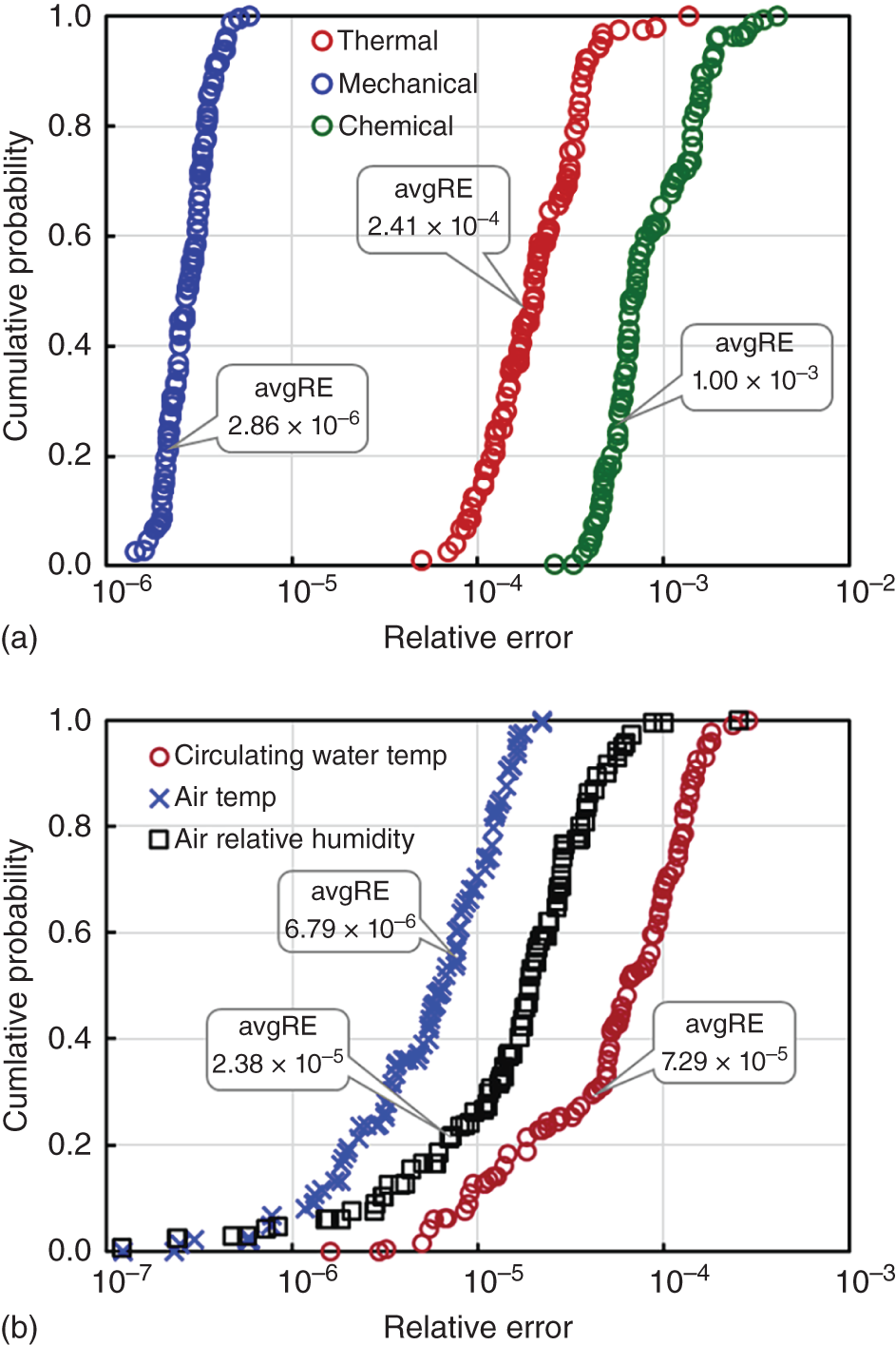
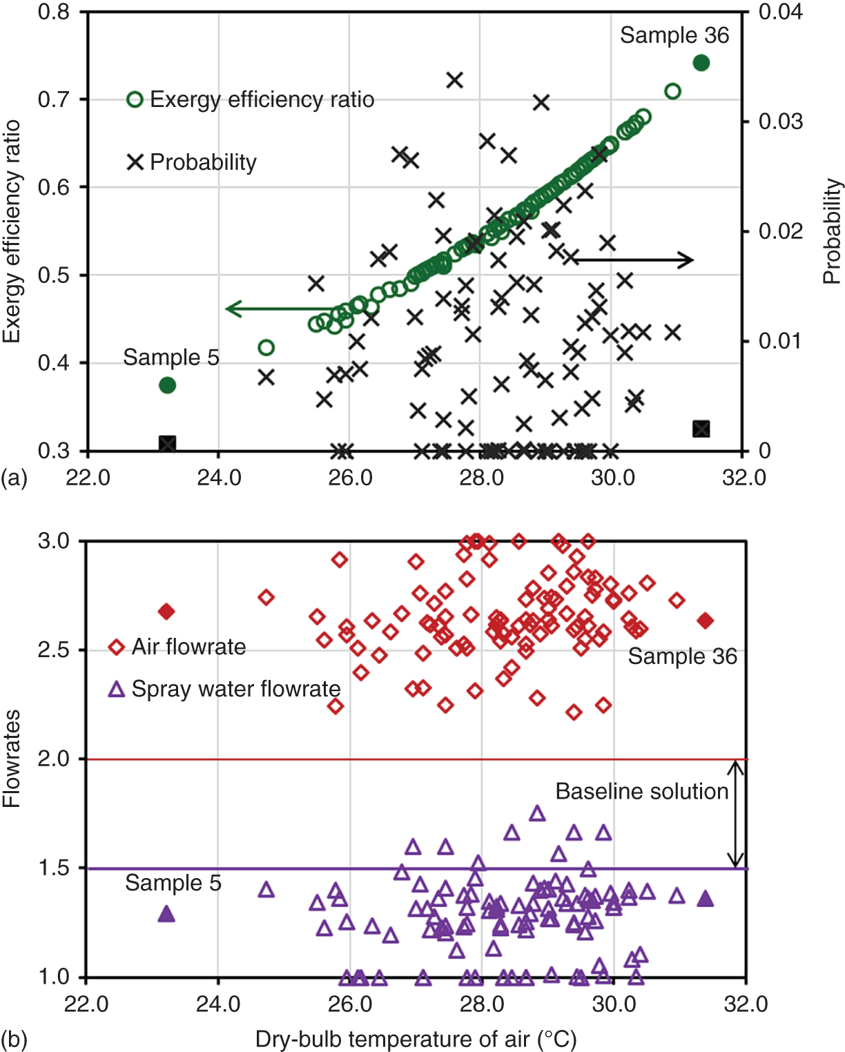
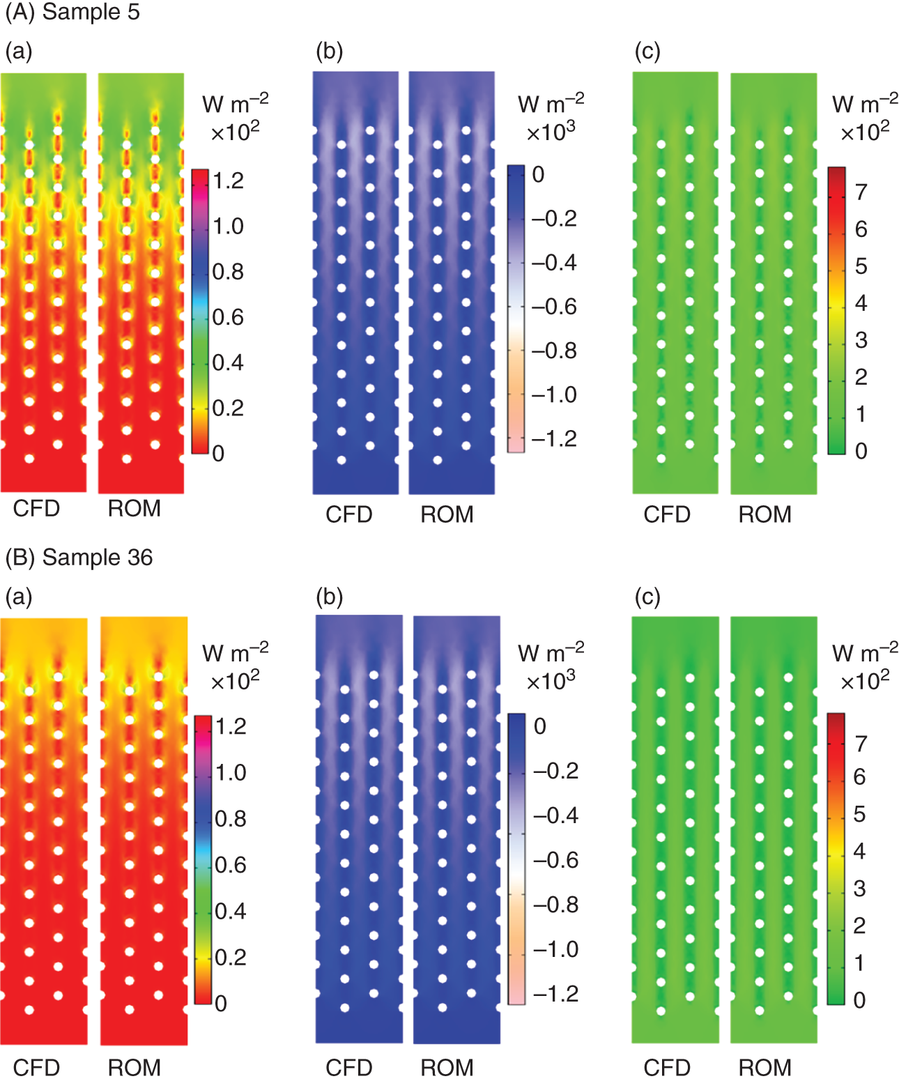
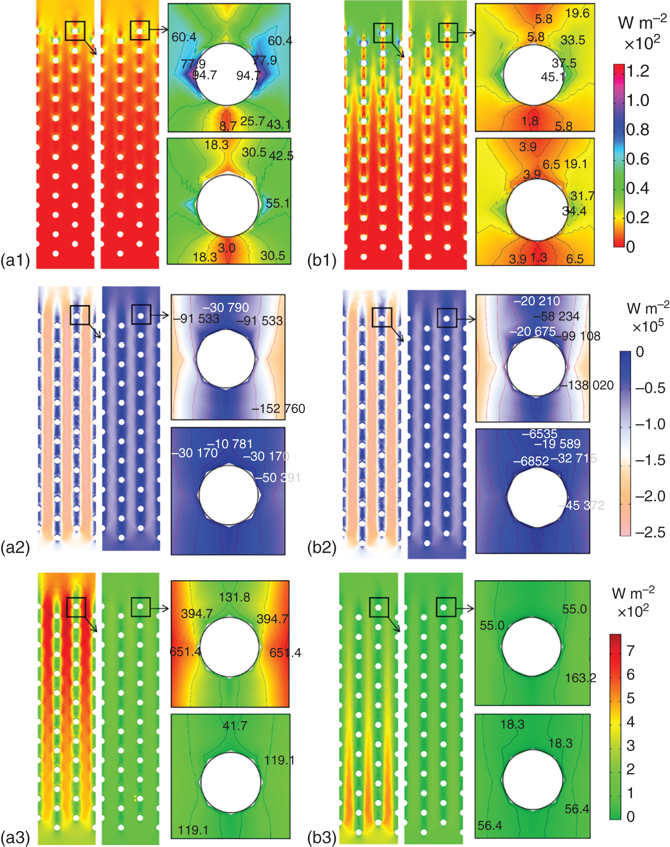
8
Data-Driven and Physics-Based Reduced-Order Modeling and Optimization of Cooling Tower Systems
8.1 Introduction
8.2 Full-Scale Physical Model of Cooling Towers

 are the static pressure and the stress tensor;
  and
and  are the gravitational body and external body forces; kceff is the effective conductivity; Djs is the diffusion flux of species js; Sh is a user-defined source term. In addition, the first three terms on the right-hand side of Eq. (8.3) represent energy transfer due to conduction, species diffusion, and viscous dissipation, respectively.

8.3 Bi-level Reduced-Order Models
 ,
,  ]T and operating variable x(2) = [
 ,
,  ]T. Similarly, the output vector y in the output space contains the values of all variables in the output streams, y = [
 ,
,  ,
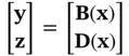
,  ]T. Note that the objective function calculation requires the results of both the input vector x and the corresponding output vector y. The state space is spatially distributed and bounded by the equipment geometry. The state vector z in the state space accommodates the values of distributed parameters at each discretized node of the mesh.
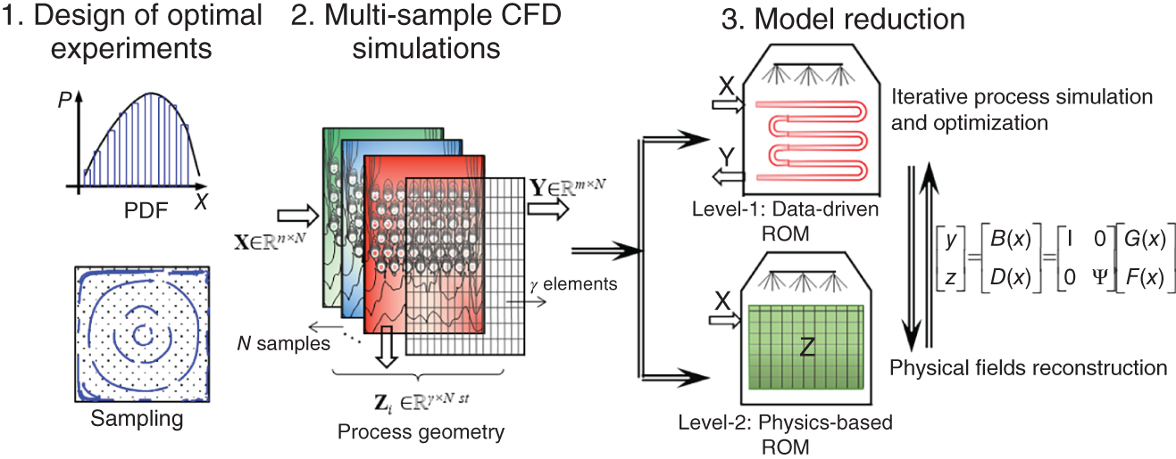
Input domain
Symbol
Unit
Specification
Control variable X(1)
Volume flow rate of air

m3 s−1
U[1.0, 3.0]
Mass flow rate of spray water

kg s−1
U[1.0, 2.0]
Uncertain variable X(2)
Dry-bulb temperature of air
Ta
oC
Uncertain variable
Relative humidity of air
φa
—
Uncertain variable
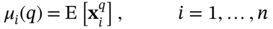
8.3.1 Design of Optimal Experiments
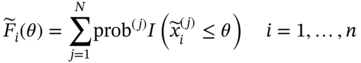
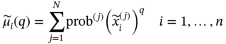
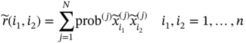
 to be specified with known expressions for its marginal distributions, moments of order q, and correlation matrix as follows:


 is an approximation of the X in the sense that
  and X have similar statistical properties. The SROM
  consists of a sample set
  with the corresponding probabilities
  , thus
  . Each sample
  contains one or multiple values, depending on the dimension of X.
 are as follows:
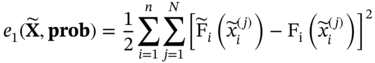
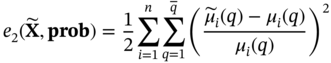
 and X in the statistical sense is represented by the distribution deviation e1, the moment deviation e2, and the correlation matrix deviation e3:
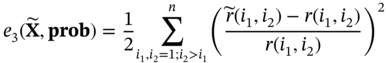
 for X with the minimum deviation can be obtained using the following optimization algorithm:
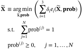
 are the weighting factors to control the contribution of each error term to the objective function. The determination of sample size N is dependent on computational considerations, and the optimal solution can be considered a good approximation of the original distribution.
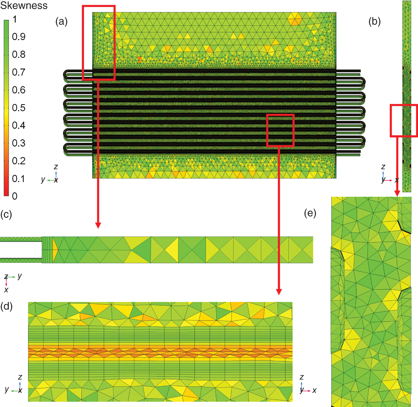
8.3.2 Multi-sample CFD Simulations
8.3.3 Model Reduction


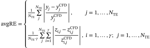
 are the results of state variables at the ith node of the mesh corresponding to the jth sample in the test set obtained from physics-based ROM and CFD models, respectively, and NTE is the sample size of the test set.
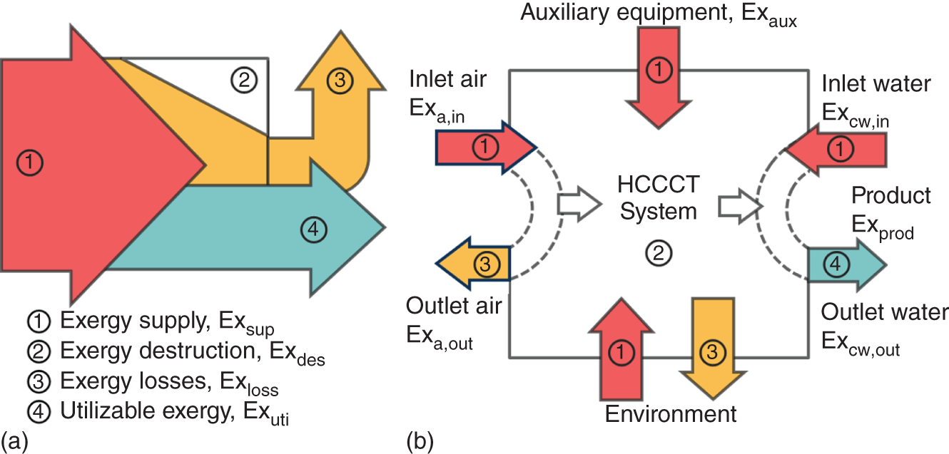
8.4 Thermodynamic Performance Indicators

8.5 Optimization Model
 is the design constraint that defines the upper outlet temperature of the circulating water for meeting the requirements of the cooling targets.
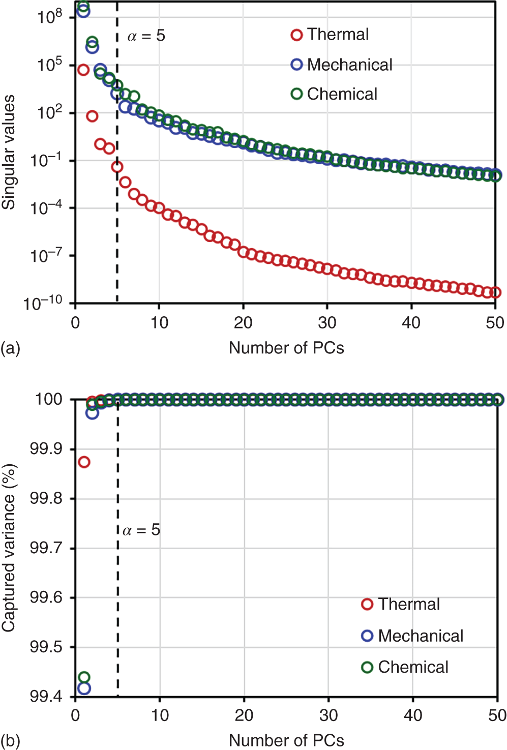
8.6 Illustrative Example
 = 23.2 °C,
  = 0.87, EER = 0.37) and Sample 36 (
 = 31.4 °C,
  = 0.57, EER = 0.74).
8.7 Conclusion
References
Data-Driven and Physics-Based Reduced-Order Modeling and Optimization of Cooling Tower Systems
(8.2)
(8.4)
(8.5)
(8.6)
(8.7)
(8.8)
(8.10)
(8.11)
(8.15)
(8.16)
(8.17)
(8.18)
(8.19)
(8.20)
(8.21)
(8.22)
(8.23)
(8.24)
(8.25)
(8.26)
(8.27)
(8.28)
(8.29)
(8.30)
(8.31)
(8.32)
(8.33)
(8.34)
(8.35)
(8.36)
(8.37)
(8.38)
(8.39)
(8.41)

(8.43)


(8.48)