Field appraisal will either close with a decision to abandon a project or a mandate to take the field into production. In this chapter, we examine the role of the geoscientist in the processes of field development, production, abandonment, and reactivation. In each of the preceding chapters, the emphasis has been placed on a description of the Earth using static data. This chapter is different. Static data are generated during production, but many of the new data available to the geoscientist and reservoir engineer are dynamic (production) data. These dynamic data are commonly available in time series. They include production profiles for wells, fluid pressure data through time, and fluid composition data collected during production. Production geoscience and reservoir engineering are intimately linked; as a consequence, field production teams commonly comprise a mixture of geoscientists and reservoir engineers. Another profound difference that separates the way in which geoscience is used in production from that in exploration is the timescale involved. It can take years for acreage to be acquired, seismic surveys shot, prospects identified, and exploration wells drilled. In such situations, the mistakes that geoscientists make may never catch up with them. They will be long gone onto the next exploration job before their poorly considered prospect is drilled and proved dry. Curiously, the same seems not to be true of success. For one of us, as a young geologist joining BP in the early 1980s, it seemed that all of the older generation in the company had a personal hand in discovering the giant Forties Field 10 years previously! However, we digress; production geoscience allows no such luxuries with time. In the most intense of operating situations, it may be necessary to plan a new well every two weeks and have the wells drilled within a few weeks of planning. Such rapid testing of one’s understanding of field geometry, fault distributions, and reservoir architecture and quality can be very exciting (or demoralizing). Moreover, the expectation at the production stage is that the wells will be successful. It is not so easy to hide behind a failure when the pre-drill probability of success was 80%, compared with an exploration prospect at 20%. Field development is covered in Section 6.2, production in Section 6.3, and changes to reserves – be that through revisions, additions, or field reactivation – in Section 6.4. It will become clear as this chapter unfolds that the discovery of an oilfield can be ascribed to a specific point in time, but no such temporal definition can be made for the point of final depletion of a field. Abandonment of a field is driven by economic criteria. At the point of abandonment the field still contains petroleum; it is just uneconomic to extract it. This fact leads to the possibility that changing fiscal regimes, increases in the oil price, the development of new technology, and reductions in operating costs can cause old fields to gain new leases of life and abandoned fields to be reactivated. The so-called “stripper wells” of North America are a case in point. These wells produce minuscule quantities of petroleum, measured in barrels per day but, during periods of high oil price the wells become economic and production is restarted, only to be shut-in again as the oil price falls. Many of these wells are exceptionally old, and because the fields repressurize during periods of low oil price (because they are shut in), recovery factors can often be very high indeed (more than 60%), something that can rarely be achieved in expensive offshore situations. The process that links appraisal and production is called development. For petroleum accumulations that are offshore, development is a distinct phase that accompanies construction of the offshore facilities. For an onshore field, appraisal, development, and production can form an overlapping spectrum of processes that take a field from discovery to peak production. This is because, in many land locations, it is possible to produce and sell oil soon after discovery. In such situations, development might reasonably be taken to cover the major period of well drilling between discovery and plateau production. Appraisal of an oil- or gasfield has delivered a measure of petroleum in place. At the onset of development, extensive modeling of the reservoir will have been completed to give an estimate of how much oil or gas is likely to be recovered and how many wells will be needed. However, such modeling of the reservoir will have used little or perhaps no dynamic data. For example, many of the recent field developments in the deep-water Gulf of Mexico were not production-tested during the exploration or appraisal phases. Companies are reluctant to test such wells because of the high expense. Instead, analog data are used to predict the flow characteristics of the field. This is a high-risk strategy. A model, life of field, production profile is shown in Figure 6.1. It is divided into three phases: production build up, plateau production, and decline. During the phase of decline much effort is put into finding additional reserves. Such reserves are likely to include improvements in recovery from the original field as well as tie backs of satellite fields. All oilfields will produce gas as well as oil and many will also produce water (Figure 6.2). This first production forecast is of particular importance for the design criteria for the production facilities. The estimated plateau oil production rate will naturally define the size of the export facility for the oil. The estimate of gas production in an oilfield will be used to determine whether a separate gas export facility is required, whether compression is required for gas reinjection, or if there is just sufficient gas for power generation at the facility. For oilfields where the production of associated gas is low, it may be necessary to import gas to the facility. The timing and quantity of water production will control how and when water handling will be installed. For example, preliminary modeling may indicate that water will not be produced for a few years after field start-up. In consequence, it may not be necessary to install the full water-handling capacity for the first day of production. The total production profile thus controls the whole design of the facilities. During the period of design and construction, much work is done on the reservoir. Indeed, it is common nowadays for production wells to be pre-drilled from a template during construction of the production facility. Such wells clearly provide a wealth of information about the reservoir. They also allow a rapid buildup of production, so as to enable an early start to paying-off the cost of development. Figure 6.1 An idealized production profile for an oilfield. Production buildup is commonly planned to be rapid, plateau stable, and decline rapid to maximize the use of the facilities. Reserves additions from satellite pools will be used to maintain the plateau. Abandonment of the field will occur before production has declined to zero, the point being determined by the cross-over between the value of the produced oil and the cost of producing it. A reduced cost of operation (OPEX) will commonly allow production to continue at economic rates beyond the initial planned abandonment date. Figure 6.2 Typical, time-dependent, fluid changes in an oilfield being produced under (a) primary gas exsolution drive, (b) gas cap drive, and (c) water drive. Pi = initial pressure, Pb = bubble point pressure, RF = recovery factor. The position of production and injection wells will be optimized using the reservoir model. The factors that will be taken into consideration are the position and strength of aquifers, the distribution of gas caps, the dip of the reservoir, its quality and the degree of layering and lateral heterogeneity, and the location and number of potential baffles and barriers to fluid flow (faults, cemented horizons, and sealing lithologies). The well positions will also depend upon the chosen method for production, which itself may in part be influenced by the distribution of the natural factors listed earlier. For example, in the super giant oilfields of the Zagros fold belt of Iran and Iraq, production wells are often placed on the crest of the fields. Many of the fields are without primary gas caps, oil columns can be measured in kilometers, reservoirs are fractured, and aquifers are poor. Without the thick oil column one would expect rapid production of water as it floods up fractures into the production wells. However, with such large fields and such thick oil columns it is possible to produce oil wells at a high rate, and it will still take many tens of years (perhaps more than 100 years) for water cut to become appreciable. In smaller fields, it may be necessary to be less cavalier about well placement. Fields deemed to have very active aquifers might need to have production wells placed not just at their crests but in lower-quality reservoir. In such situations, high-permeability conduits could cause much oil to be bypassed, such that production wells quickly run to water. This situation is a progressively greater problem as oil viscosity increases. Oil reservoirs with gas caps require a different well placement strategy. A reservoir containing a large gas cap, a poor aquifer, and an oil rim may be exploited by placing production wells low in the oil column or even at the top of the underlying water interval. However, if the aquifer is large and active, wells tend to be drilled in the lower part of the oil leg. In this instance, it is commonly easier to manage a downward migration of the gas/oil contact by injecting gas into the gas cap. If the field is to be produced using secondary recovery techniques, the position of wells for water or gas injection must also be planned. Water injection is commonly planned either as line drives or pattern floods. These terms are reasonably self-explanatory (Figure 6.3). Line drives are commonly used in dipping reservoirs, while pattern floods may be used in complex reservoirs or near flat-lying reservoirs. If a reservoir is heavily segmented, it may be necessary to treat each segment as a separate accumulation and use paired production and injection wells for each segment. In recent years, some less than obvious water-flood techniques have been tried with considerable success. In the giant Prudhoe Field (Alaskan North Slope), water has been injected into the gas cap. Because the oil and water legs are laterally separated in this low-dipping reservoir, this method has compromised neither the oil nor the gas production, but has helped to sustain reservoir pressure and thus oil production. The injected water sinks to the base of the reservoir section and then flows down dip, so displacing oil toward the production wells. Figure 6.3 Well patterns used for water drive, secondary recovery. Fields with natural gas caps are often considered for gas cap drive (Figures 6.2 and 5.52). Associated gas, that exsolved from the oil during production, can be injected into the gas cap to maintain pressure. Even in reservoirs that lack natural gas caps, gas may still be put into field crests because it is an extremely efficient displacement process, enabling production of attic oil that may otherwise be inaccessible. This technique has been used in the western panel of the Douglas Field (East Irish Sea Basin; Yaliz and McKim 2003). In the Lennox oil- and gasfield close to Douglas, wet gas (methane plus higher homologs) has been injected into the gas cap to maintain pressure (Yaliz and Chapman 2003). Preliminary analysis of the data for Lennox indicate that gravity segregation of the “heavier” components within this gas may limit gas breakthrough in oil production wells by reducing the viscosity contrast at the gas/oil contact. In some fields, a combination of water and alternating gas injection (WAG) may be chosen. The development team uses the reservoir model to determine the number of wells required. The reservoir model will also yield the expected volume of petroleum that is recoverable from each well. Although every effort will be taken to ensure that the reservoir model mimics the behavior of the field when in production, it is of course not conditioned to the actual performance of the field for which it has been built. However, after the field has been on production for some time, it will become clear just how much each well is capable of producing and the degree to which the model was able to forecast the behavior of the field. Naturally, the new production data can be used to modify or rebuild the reservoir model and so refine the forecasts for production from both individual wells and for the field as a whole. The quantity of petroleum that can be recovered from a well depends upon a range of criteria. These include the permeability of the reservoir, the viscosity of the oil, the degree of reservoir heterogeneity, well management (pressure drawdown history), the presence or absence of aquifers or gas caps, and well longevity. The most prolific wells in the world’s giant fields can deliver over 50 million barrels during their lifetimes, while the productive history of most wells can be measured in hundreds of thousands of barrels. For example, wells in the Magnus Field (UK North Sea) need to deliver on average 50 MMBO; while Helena-1, the discovery well for the Forest Reserve/Fyzabad complex (Trinidad), celebrated its 75th birthday in 1995 having delivered about 750 000 bbl. In reaching this quantity of oil, the well has been worked over about six times in its 75-year history. The ultimate life-of-field productivity for gas wells is commonly measured in tens to hundreds of billions of standard cubic feet. Most exploration and appraisal wells are vertical. Few development or production wells are vertical. A vertical or near-vertical well is the natural choice during exploration. The aim of the well will be to penetrate a primary, and possibly several secondary, target horizons. A vertical well cuts across the stratigraphy. It is easier to plan on the sparse seismic data commonly available during most exploration programs than would be a well with more exotic geometry. A vertical well will also allow collection of data such as pressure gradients and it will possibly penetrate fluid contacts (gas/oil, gas/water, and oil/water). Quite clearly, a development/production well has quite different requirements. The aim for such wells is to produce as much petroleum as possible, and to produce that petroleum at economic rates. This can be achieved in a variety of ways, although ultimately the effect is much the same; optimization of permeability × height (measured in millidarcy-feet, mDft, or millidarcy-meters, mDm). Such optimization may mean that the field has many vertical wells (Figure 6.4a) or a few high-angle or horizontal wells (Figure 6.4b). The decision on the type of well to be drilled will be a function of the location, the petroleum distribution, cost, and the reservoir properties. In an onshore location, vertical wells may be easy to locate, shallow, and cheap to drill. In such situations, it would be perverse to try to drill expensive and complex geometry wells. Offshore, the situation is different. It is rarely possible to have lots of wellheads scattered over a large area, except in shallow lakes and seas subject to mild weather conditions (e.g. Lake Maracaibo, Venezuela; the Gulf of Paria, Venezuela/Trinidad). In offshore settings such as the Gulf of Mexico, offshore West Africa, and the North Sea, wellheads will be clustered at the production facility (Figure 6.5). Well tracks will be deviated away from the facility location to cover the productive area of the field. The angle of the wells as they pass through the reservoir can vary from vertical to horizontal. As discussed earlier, high-angle and horizontal wells will tend to be more productive than vertical wells insofar as they have longer sections in reservoir than do equivalent vertical wells. The choice of high-angle versus horizontal is commonly made depending upon the vertical heterogeneity of the reservoir. Strongly layered reservoirs in which there are barriers to vertical fluid flow may not benefit from horizontal wells – or, more properly, those that are parallel to the stratigraphy – because the barriers will prevent petroleum from being produced from horizons not specifically penetrated by the wellbore. In such instances, it is commonly the practice to drill wells that cross-cut the reservoir stratigraphy. Figure 6.4 Vertical versus horizontal wells (contrasted development methods) for the Argyll and Foinaven fields, UK continental shelf. (a) The Argyll Field was developed with vertical and near-vertical wells from a floating facility during the 1970s and 1980s. Each well penetrated all reservoir horizons, while commonly the wells were completed in just one horizon. (b) The panel map and development well locations for the Foinaven Field, UK continental shelf. The wells are drilled from two centers (DC1 and DC2), individual, high-angle wells targeting specific reservoir, sandstone lobes. Development wells were drilled during the late 1990s and early 2000s. Source: From Carruth 2003. Reproduced with permission of Geological Society of London. Source: Carruth 2003. Reproduced with permission of Geological Society of London. High-angle and horizontal well technology was developed during the 1980s. The product of the 1990s is the multilateral well. In such wells there are two or more branches in the reservoir section. Clearly, although such wells are complex to drill, much money is saved in drilling the top-hole section. It is drilled only once for each multilateral cluster. An example of multilateral wells being used in field development comes from the Lennox Field in the East Irish Sea Basin (Figure 6.6; Yaliz and Chapman 2003). The field is a broad domal structure, with a thick gas cap of about 700 ft and a thinner oil leg of about 150 ft. The unmanned platform lies approximately above the center of the field, from which wells are drilled vertically downward toward the field, before being deviated to horizontal within the oil leg. The field contains one trilateral well drilled in the east and south and several bilateral wells. Figure 6.5 Clustered wellheads and radiating wells beneath the two production platform locations. Source: Courtesy of Dynamic Graphics Earth Vision model. Figure 6.6 Multilateral wells in the Lennox Field, East Irish Sea Basin, UK. Well L6/L6Z is a bilateral well drilled in a partial spiral beneath the platform, while L8/L8Z/L8Y is a trilateral used to exploit the southern part of the field. All wells are essentially horizontal within the oil rim to the Lennox Field. Source: Yaliz and Chapman 2003. Reproduced with permission of Geological Society of London. Wells can be divided into three broad categories; production wells, injection wells, and utility wells. We have already covered production wells. Injection wells may be required for either water or gas, depending upon the recovery method used or the field. Utility wells can include those drilled as a source of water for injection, those drilled such that produced water and cuttings can be disposed of, and those used for observation. The primary purpose of injection wells, be they for water or for gas, is to maintain the pressure in the reservoir as petroleum is extracted. The efficiency with which the water or gas will sweep oil from the reservoir is also important. Water injection will be of little value in a field if the injected water runs from injection well to production well and bypasses much of the oil in the reservoir. Most oils are more viscous than water and the problem is exacerbated as the viscosity contrast increases. Thus attempts are made to place injection wells where pressure support can be maximized and the potential for water breakthrough minimized. Whether or not this can be achieved will be determined by the segment size of the field and the permeability heterogeneity. Clearly, it is best to avoid high-permeability intervals with injection wells, as these can often be conduits direct to production wells (Figure 6.7). The injection of cold water into hot rock can lead to thermal fracturing as the rock shrinks around the wellbore area. The direction of fracture propagation can be determined by measuring the local stress field in the subsurface. Clearly, fractured rock will allow greater injectivity for a given injection pressure. This natural phenomenon is commonly used to help injectivity in hot and deep reservoirs that have low matrix permeability. The design of injection wells, like that of production wells, has become highly sophisticated. For example, paired groups of multilateral production and injection wells are being used to produce oil from poor-quality carbonate reservoirs in the Middle East. In this particular example, productivity was improved by two orders of magnitude compared with the production rate in the original, vertical wells. This has allowed development of hitherto uneconomic oil. All of these injection wells need to be designed by a team that includes drilling engineers, reservoir engineers, and petroleum geoscientists. Utility wells, be they for injection of produced fluid waste or cuttings or for source water, tend to be simple and are likely to be near vertical. Although such wells will be simple in geometric terms, the geologist will be involved in determining their position in much the same way as would be required for production and injection wells. For example, the distribution of Paleocene submarine-fan sandstones overlying the Jurassic-age reservoir of the Gyda Field (Norwegian North Sea) was studied from the point of view of cuttings injection. Observation wells are rarely drilled in their own right, except to monitor flood fronts in enhanced oil recovery (EOR) pilot projects. More often, pressure gauges are inserted in an old wellbore. In addition to determining the best locations for production and injection wells, it commonly falls to the geoscientist to identify potential drilling hazards for a well. It is most important for the geologist while planning a well to identify possible sources of danger to human health. In many instances, the singularly most important and abundant shallow hazard is gas (methane). It is most usual to conduct high-resolution (seismic) site surveys to enable identification of such gas. Other hazards include seafloor instability, shallow water flows (especially in deep-water) and gas hydrates, often difficult to detect from conventional seismic data. Mobile mudstones and those that are chemically unstable with respect to drilling fluids are also commonly mapped. Similarly, hard horizons such as flint layers tend to be identified and their abundance calculated. Once the potential hazards have been identified, the drilling engineer can plan to minimize their effect. This may be manifest as a decision to change the drill bit before entering hard lithologies, to manage the mud weight in sensitive formations, or to modify casing schemes (the process of stabilizing an open hole by cementing a pipe in place). Figure 6.7 A sketch showing the control of permeability profile in a well on the injected water-flood front. (a) A downward decrease in permeability results in an even flood front, with the denser water slumping to the base of the sandstone, so displacing oil from the lower-quality rock. (b) The high-permeability conduit at the base of the sandstone promotes water under-run and early breakthrough of water into the production well. The process that takes place between the drilling of a well and the production of petroleum from it is called completion. The type of completion can vary from the most simple – open hole – to rather more sophisticated methods using slotted liners, wire mesh screens, gravel packs, and fracture stimulation methods. The main aim of completion is to optimize petroleum production while maintaining the integrity of the wellbore. In many instances, the technology required to stabilize the wellbore has a detrimental effect upon the productivity. For example, in poorly consolidated formations it may be necessary to place a gravel pack (a sheath of clean, monodisperse sand, or glass beads) across the producing interval, so as to reduce or eliminate the tendency for the well to produce sand as well as petroleum. Clearly, in placing a gravel pack across the production interval, the permeability in the wellbore has been compromised. The role of the geoscientist is to describe the rocks penetrated by the well in terms of their physical properties, such as permeability, the degree of consolidation or cementation, and the natural stress regime. Well-stimulation technology is designed to improve the near-wellbore permeability. Such stimulation may be either through physical or chemical methods. Acid washes can be used to dissolve minerals in the near-wellbore region. Hydrochloric acid is used for carbonates, while hydrofluoric acid may be used for low-permeability sandstone formations. Apart from the intrinsic health hazards of using such acids, work is also required on the reservoir formations prior to acid treatment, to determine their suitability for such treatment. For example, direct treatment of the Rotliegend Sandstone of the North Sea’s Southern Gas Basin with hydrofluoric acid can result in reduction of permeability, as the hydrofluoric acid reacts with calcite and dolomite to produce insoluble calcium fluoride (fluorite). In consequence, such sandstones are commonly pretreated with hydrochloric acid to remove calcium carbonates before the hydrofluoric treatment. Problems may also be encountered with the production of iron hydroxide gels following acid treatment. It is therefore important to have a mineralogical analysis of the formation prior to any chemical treatment. Physical stimulation of reservoirs commonly involves fracturing. In this instance, fractures are created hydraulically, using a suspension of tough beads in a proppant gel. The mixture is injected into the formation until the rock fractures. The mix of proppant gel plus beads migrates along the fractures. At the end of the fracture process, the pressure is reduced but the fractures are kept open by the injected beads. The proppant gel is then broken down. This may require further chemical treatment. Alternatively, the proppant may be designed to degrade naturally. Quite clearly, the important geoscience work to perform prior to any “frac pack” treatment is that of analyzing the local stress regime. The ideal fracture geometry is one that is parallel to the wellbore, rather like a pair of “Mickey Mouse” ears (Figure 6.8). This can normally be achieved when the principal stress direction is vertical (gravity). However, in neotectonic areas the principal stress direction may not be vertical, and in consequence the fracture may open up perpendicular to the wellbore. This leads to minimal improvement in near-wellbore permeability (Figure 6.8). Indeed, this is believed to have happened when attempts were first made to reactivate the Pedernales Field in eastern Venezuela (Jones and Stewart 1997): a wrongly designed frac-pack is thought to have led to complete loss of productivity in the first of the reactivation wells drilled. Formation damage is the inadvertent and opposite effect to well stimulation. Permeability is reduced and the flow rate of the well diminishes or is stopped altogether. Two categories of mechanisms can be responsible for formation damage; reduction of absolute permeability, or reduction of relative permeability in the near-wellbore region. Although the overall effects of formation damage can be categorized simply into one of these two mechanisms, the individual causes are multifarious and a whole array of individual terms has been developed to describe various situations. Just a few of these are water block, condensate block, fines migration, asphaltene drop-out, and scaling (mineral precipitation). Some effects may be cured or reduced by remedial action, but the best option is to reduce the likelihood of the problem in the first place. As will be clear from some of the terms described above, formation damage results from the physical effects on the reservoir and fluids caused by drilling, or by the interaction between the drilling fluids and formation fluids or reservoir minerals. Figure 6.8 Artificial fracturing of wells can stimulate production by increasing the effective contact area between the wellbore and the formation. Under normal hydrostatic or even normal compactional overpressure, the fracture surface radiates from the wellbore as two “ear-shaped” surfaces. However, in situations in which the principal stress is horizontal and the minimum stress vertical, the fracture is horizontal, and in consequence the surface area of fracture in the wellbore is minimal. The degree of damage to a well is referred to as the “skin factor.” This skin effect can be considered as a rate-proportional steady state pressure drop, given as a product of a flow-rate function and a dimensionless skin factor (Archer and Wall 1986). The numerical value of the factor is only a semiquantitative measure. Nonetheless, such numbers do help to describe formation damage. For example, for a vertical, unfractured, and undamaged well, the skin factor would be zero. As the degree of damage increases, so does the skin factor. Skin factors of less than about five indicate a little damaged well. Skin factors reported as many tens or even hundreds are obtained from severely damaged wells. It is possible to calculate a negative skin factor. This can be real, insofar as it is a product of a naturally or artificially fractured well, or simply a product of the calculation, as can be the case in a high-angle or horizontal well. In both instances, it implies that the flow into the wellbore will be greater for a given pressure drop than would be the case in an undamaged, equivalent vertical well. Absolute permeability reduction occurs when pore throats in the near-wellbore area are blocked. Such blocking can occur when fines such as clay minerals become detached from their host grains and migrate toward the wellbore. Both chemical interaction between the drilling fluids and the rock and the physical effects of fluid flowing from formation into the wellbore may be the cause. The same absolute reduction can occur when drilling fluids and formation fluids react to produce insoluble precipitates. A particularly dramatic example of such formation damage occurred when the discovery well of the Miller Field (UK North Sea) was drilled in December 1982. One of the authors was involved in the detective story associated with tracking down the problem of a nonproductive well test on the Miller discovery well. The Miller reservoir is almost pure quartzite and is one of the cleanest sandstone reservoirs known (Gluyas et al. 2000). However, on test the discovery well failed to flow at an appreciable rate. The initial reaction of the drilling, completions, and testing teams was that the rock was of poor quality (permeability). This was not compatible with either sedimentological or core analysis data. The porosity was known to range between about 13% and 25%, and the absolute permeability was measured in hundreds of millidarcies and darcies. Routine analysis of the rock using a scanning electron microscope showed that although it comprised quartz-cemented quartz grains, many of the pores were partially filled with patches of a microcrystalline solid. Coincident with the work on the Miller discovery well, an EDAX (X-ray elemental analysis) facility had been fitted to the microscope. The microcrystalline mass was found to contain barium and sulfur. At first, it was thought that this barium sulfate (barite) was a contaminant from the drilling mud. However, this proved not to be so. The formation waters in Miller were found to contain between 1000 and 2000 ppm of dissolved barium, and the exploration well had been drilled with a seawater-based (sulfate-rich) mud system. Barium and sulfate had reacted to yield a near-impermeable membrane around the wellbore. But for this work on formation damage, a cooperative venture between geoscientists and completion engineers, the barite problem might never have been properly appreciated, the research work on scale prevention not initiated, and the full quality of the Miller reservoir never recognized. Reduction of absolute permeability can also occur when drilling fluid filters into the formations and solids are deposited around the wellbore. Such formation damage is commonly very difficult to remove or reduce during the well-completion process. Reduction of absolute permeability can also occur as a result of precipitation of asphaltene from the reservoired oil. Such precipitation can occur in some oils when the pressure is reduced. This is a very common problem in production strings. Here it can be removed, albeit with difficulty, by scraping the production string or giving it a chemical wash with a nonpolar solvent such as toluene or xylene. However, if precipitation occurs in the reservoir close to the wellbore, amelioration of the problem can be near impossible. The well may have to be abandoned. The propensity for asphaltene precipitation needs to be studied by the geochemist, using fresh oil samples taken, if possible, at reservoir conditions. Asphaltene precipitation, both natural and induced, is a problem in parts of the El Furrial Province in eastern Venezuela. Relative permeability reduction is a product of having several phases of fluid (gas, oil, and water) in the near-wellbore region. The relative permeability to the desired phase, usually oil, can be impaired or even reduced to zero by the presence of another phase. The use of water-based drilling fluids can in some reservoirs lead to so-called “water block,” in which only water can be produced back into the wellbore. A similar situation can be induced if the pressure drawdown during testing and production causes gas to break out in the reservoir. Formation damage can occur in injection wells just as easily as in production wells. The former leads to a loss of injectivity and the latter to a loss of production. Although here we have concentrated on near-instantaneous effects caused by drilling, formation damage can progressively reduce the productivity/injectivity of a well. Particularly acute problems are commonly encountered once injection water starts to break through into production wells. Many formation damage problems can be avoided or minimized by appropriate geoscience work on formation mineralogy, formation fluids, and the physics of the reservoir and fluid system. In the preceding chapters, a variety of well logs and the data obtained from them have been described. These data have in all instances been static data, rock properties, and fluid properties. However, it is also possible to take measurements in flowing production and injection wells. The aim of such measurements is to obtain information on the rate of fluid flow, the type, and locations of different fluids as they enter the wellbore and where fluids are flowing (inside the well casing or behind pipe). It is also possible to measure pressure data from wells during flow periods or pressure changes when a well is not flowing. In this section, we will concentrate on the geologic information that can be obtained from such logging and well testing. Such data can help the geoscientist to improve his or her description of the near-wellbore region, as well as yielding data on the reservoir architecture and the proximity to barriers such as faults. Production logging methods are highly varied. They include mechanical devices (spinner surveys) and radioactive methods to detect fluid flow in the wellbore. The fluid type can be measured using density tools or fluid capacitance instruments, in which the dielectric properties of the fluid are used to differentiate between petroleum and water. Temperature data are also very useful in allowing the identification of flowing and nonflowing units within producing wells, injecting wells, and even shut-in wells. The spinner type of survey uses an instrument that contains an impeller. As the instrument is pulled up the well, across the flowing reservoir interval, the impeller spins ever faster in response to the flow into the wellbore. If particular intervals are not contributing to flow, then the rate of spin does not increase as the tool passes across them. In an undamaged well, with all zones contributing, there will be a close match between a composite permeability height plot for the interval and spinner results. The radioactive devices depend upon the injection of a slug of radioactive material into the wellbore. The radioactivity is then measured across the reservoir interval and the results may be interpreted in terms of flowing and nonflowing intervals. Given the obvious environmental and health issues of such a process, the application of such technology is commonly limited to injection wells. The capacitance and density methods allow identification not just of petroleum versus water but of where the different fluids are entering the wellbore. In a geoscience context, such information will enable improved reservoir description, the application of which may help to avoid water inflow in subsequent wells, as problem intervals need not be perforated. In much the same fashion that mechanical spinner tools can be used to measure fluid flow, so too can temperature response tools (Figure 6.9). For example, in an injection well, cold injection water is introduced into a hot formation. If a particular horizon is accepting most of the injected water, then it will be cold relative to those horizons in which injection is limited. In much the same way, temperature data in a shut-in well can help to identify cross-flow between formations. Figure 6.9 A temperature log from a production logging suite. Below the perforations at 10 115 ft there is a column of water in the well, extending to 10 200 ft. Except for some minor water production at 10 115 ft, the water column is inactive; therefore the portion of the temperature log below 10 120 ft has a slope like that of the geothermal gradient. Both the temperature and fluid density decrease significantly at 10 115 ft, which indicates substantial gas production at that depth. Source: From Western Atlas 1982. Pressure data from wells are used to define local and field-average reservoir pressures. Such data, when combined with production information on petroleum and water, and with fluid and rock property data, can be used to calculate the petroleum in place and the expected recovery factor. Unlike measurements based upon core or well logs, which only yield direct data from within or close to the wellbore, the depth of investigation of time series pressure data can encompass an entire field or field segment. Pressure tests (e.g. RFT™s and MDT™s) can be made in flowing wells in addition to static wells (Chapter 2). Data from such tests can be used to indicate the boundaries to individual flow units, barriers to flow, and compartments in the reservoir. The interpreted data from the pressure tests can then be used to aid field development design. Pressure data from wells, rather than individual formations, may be obtained in a variety of situations. Data can be collected during constant production from a well (pressure drawdown), while a well is shut in (pressure buildup), during multiple-rate flow periods, in one or more shut-in wells while producing from another, in injection wells, and in drill stem tests (DSTs). The essential feature of all of these different situations in which pressure is measured is that a time series of data may be obtained. The temporal response of the field to a pressure disturbance is being measured. We will concern ourselves here with the description of such test data. The mathematical background is given in Matthews and Russell (1967). Reasons that pressure buildup tests tend to be performed more often than drawdown tests include: (i) during buildup the well is responding only to the natural restoration of pressure and is not under the influence of “man-induced” flow, and therefore the more subtle pressure changes are likely to be captured, and (ii) a combination of legislation and much greater awareness of environmental issues means that waste emission during testing of exploration and appraisal wells (flaring) is minimized. As a consequence wells tend to be flow-tested for short periods and then the pressure is allowed to build up over a few days. Whether during drawdown or buildup, the pressure change through time can be divided into three periods, characterized by different pressure change behavior. In the period immediately following the pressure disturbance (test), the wellbore pressure is unaffected by the drainage boundaries of the well and the pressure buildup behaves as if it were occurring in an infinite system. This interval of time is often referred to as the “transient period.” At some time later, the influence of the nearest boundary is seen in the wellbore pressure response. Other boundaries may then be observed during this so-called “late transient period.” Finally, the pressure buildup (or drawdown) reaches steady state (the rate of change of reservoir pressure is constant with time) once stabilized flow conditions have been established. The change from transient to steady state depends in particular upon reservoir geometry, reservoir compartmentilization, porosity, and permeability. Ideal behavior (Figure 6.10) is rarely achieved, and a number of techniques have been developed for analysis of the data in the absence of constraining geologic information (Figure 6.11). Naturally, the corollary is that when combined with geologic data (fault distributions, reservoir pinchout maps, and fluid composition data), the pressure data provides a very powerful tool for reservoir description. Most tests are performed at a constant production rate. However, it is possible to derive much of the same data by performing tests on a well that is subject to multiple-rate flow periods. This is particularly common on gas wells, which may require such testing to satisfy regulatory bodies. This method is also used on wells where a shut-in prior to a drawdown test or for a buildup test may not be economically desirable. Figure 6.10 A pressure drawdown test, showing the time ranges for which various analysis methods are applicable. Source: Adapted from Matthews and Russell 1967. Figure 6.11 A summary of well/reservoir responses to testing in different reservoir systems. Source: Adapted from Archer and Wall 1986. One further category of well test, the interference test, deserves particular mention. In a single well test, although the pressure buildup information may be highly accurate, it is commonly difficult to interpret the data in geologic terms because it is scalar: the distance to boundaries may be observed, but the direction to those boundaries is not known. Even when high-quality geologic data are available, it may not be easy to identify the likely geologic features responsible for particular effects on the pressure buildup. The value of time series pressure data can be maximized in interference tests. In such tests, a well is put on production or subject to injection while one or more surrounding wells are shut in, with pressure gauges installed. The effects of the production or injection can be recorded in the surrounding wells. Clearly, the response in these wells will be delayed relative to initiation of flow in the production/injection well. Factors that will influence the response time and response effect are distance, permeability, connected porosity, and directional reservoir flow patterns. That is, when combined with the geologic data, it should be possible to describe the location and nature of baffles and barriers to fluid flow and the permeability anisotropy of the reservoir system. Where pressure data are not available, it may be possible to use the production history of wells to effect a similar analysis of reservoir performance behavior. The technique is simply one of observing the effects on existing wells when a new well is brought on stream. The method is particularly useful when applied to old fields with many closely spaced wells. Often in such situations, the production data and well histories are the only recorded data for the field. Such production data are a valuable tool for the geoscientist. The petroleum production rate obtained during a well test is an important indication of how the well, and indeed the field, will behave when on production. An important derivative of a production test is the productivity index (PI). This is because the actual production rate in a test varies as a function of the pressure drawdown imposed upon the reservoir as well as the intrinsic properties of the reservoir and its oil. The PI is thus a measure of the performance of the reservoir, normalized for the pressure difference between the reservoir and the wellhead (drawdown): where q is the rate of production, in m2d−1 or bd−1; The estimation of PI from static data is possible using permeability, reservoir thickness, and oil viscosity data (Case History 6.6). However, this tends to be only an approximation, since the PI is commonly rate dependent. Reservoir description from production data is an essential part of maintaining production from a field on plateau and extending the life of a field in decline. There are few things about which there can be certainty when producing a field, and one of those certainties is that the field will not perform as the development plan suggested it would! The main factors of interest to the production geoscientist are establishing what petroleum has been produced from where, and how both petroleum and water reach the production wellbore. These two pieces of knowledge will allow the geoscientist, working with the reservoir engineer, production engineer, and drilling engineer, to target unswept oil and possibly reduce the unwanted water flowing into the production wells. Moreover, during production, information arrives very quickly and in large quantities. Most fields have many tens or even hundreds of wells and there may also be many layers within the reservoir. The production geoscientist needs to be able to capture and assimilate the data and then use it to guide further production of the field. In consequence, graphic and pictorial methods are often used to synthesize the mass of data into something understandable. In fields with many tens, hundreds, or even thousands of wells, it will not be possible to understand the full details of field performance without a lot of work, which takes a lot of time. In such circumstances, time is often short and as a consequence it is commonly necessary to study just the anomalous wells, those that either over-perform or under-perform. In doing so, it may be possible to understand about 80% of the field performance characteristics by working on about 20% of the wells. A very simple analysis of production data is to plot produced volumes on a map of the field. Bubble plots (Figure 6.12) can be constructed simply, using the proportionality between the area or radius of the bubble and the produced volume. A slightly more sophisticated method would be to overlay the bubble plot on a contoured petroleum pore-volume map for the field. In a highly layered reservoir in which individual layers are completed sequentially, it may be appropriate to produce a map for each layer. Derivatives of the same basic method would be to plot cumulative water volume, time to water breakthrough, or changing gas to oil ratio. From any and all of these maps, it will be possible to visualize how the field is behaving through time. The spatially mapped production data can be used to identify areas of poor recovery. By comparison of the production data with the static reservoir description, it could be concluded that such areas are poor because the intrinsic oil volume is low (a thin reservoir or low porosity) or because of poor production characteristics. The course of subsequent action could then be either to do no more if there is insufficient petroleum to merit further production, or to attempt to stimulate the poor production. Another possibility is to examine the recovery factor of areas with high cumulative production. These areas could form targets for new wells. This approach was used in the reactivation of the Pedernales Field in eastern Venezuela (Gluyas et al. 1996). The best-producing wells in Pedernales had delivered 5–8 million barrels of oil, and yet a simple calculation on well spacing and total reservoired volume indicated that even in the field segments penetrated by the high-productivity wells, recovery was still below 10%. The old wells were not usable, but new infill wells in the same field segments gave excellent performance. Figure 6.12 Field production data represented using a “bubble” plot. The diameter of the circles is proportional to the volume of oil (or gas) produced. Such maps can be used to identify high- and low-productivity areas and relate well performance to underlying geology. Information on the performance of specific horizons in a well can be obtained from production logging (Section 6.2.7) or alternatively on drilling new wells. Wells drilled after start-up of a field may show modified petroleum and pressure distributions (Figure 6.13). If the well cuts a petroleum/water contact, the contact might have moved (upward) compared with the original position in the virgin reservoir. There may also be intervals above the petroleum/water contact that have become water bearing, with only residual petroleum saturation as a result of petroleum production. Pressure profiles in the new wells may indicate horizons that are more or less fully depleted. These data can all be used to help construct a more robust description of the reservoir architecture than is possible from static (geologic) data alone. The utility of pressure test analysis in wells as a reservoir description tool has already been covered in the previous section. Analysis of produced waters can also provide insight into the way in which the field’s aquifer behaves during production and the permeability anisotropy of the reservoir. Bulk fluid chemistry can be of some use, although methods using either injection of tracer chemicals or naturally occurring stable isotopes of hydrogen and oxygen tend to produce less equivocal data, since they are unaffected by water–rock interaction. Coleman (1998) reported on water production data from the giant Forties Field (North Sea). Unfortunately, no isotope measurements were made before field start-up. Nonetheless, Coleman was able to demonstrate that there were two different naturally occurring waters in the oilfield, produced in different places from different layers and at different times. In addition to these natural waters, there was also the injection water that eventually broke through to the production wells. The use of all of these data helped to improve the reservoir description, and in so doing helped to extend production from the field. It is important that the geoscientists and those working in other disciplines share a common understanding of the petroleum accumulation under development and production. Most fields are complex, be that complexity in structure, reservoir architecture, or fluid flow behavior. Reservoir visualization techniques provide an opportunity for all of the technical and managerial disciplines to share a common understanding of the field. Most of the visualization techniques that we report in the following paragraphs have already been mentioned earlier in the book, usually in the context of the way in which they are used as part of the geoscience component of exploration, appraisal, and development. Here, we will concentrate on the visualization characteristics. For technical and managerial staff without specific geoscience training, it can be very difficult to create a mental picture of a reservoir from scattered seismic lines and a couple of well logs. Yet, clearly, such interpretations are part of the geoscientist’s skill base. Three-dimensional seismic displays, geocellular models, virtual reality simulations, and outcrop analog data can all help to share information between disciplines because of their highly visual nature. Readily available software now allows 3D seismic data to be displayed as a data cube (Figure 6.14). Such data cubes can be rotated in any desired direction, sliced in any desired direction, and surfaces or individual seismic lines peeled away. Short movie sequences can be constructed to view the cube of data as surfaces (vertical or horizontal) are stripped away. Data cubes can be made to be semi-transparent, with perhaps only peaks and troughs appearing as opaque voxels. When displayed in this way, it is possible to look inside the data volume. All of these types of seismic data display allow trap configurations and structural elements to be appreciated. Figure 6.13 Well logs and pressure data from a well in the Brent Field, UK continental shelf, to show the subdivision of the Brent reservoir into geologic formations and petroleum engineers’ “cycles” and “units.” The RFT™ pressure measurements show pressure differences between and within cycles, which have developed during production as a consequence of vertical pressure barriers or baffles within the sequence. Source: Adapted from Bryant and Livera 1991. Figure 6.14 A 3D seismic data cube, showing two orthogonal cross-sections and a time slice. Source: Image supplied by Schlumberger, Gatwick, UK. (See color plate section for color representation of this figure). The same sort of image manipulation methods as applied to seismic data may be applied to geocellular models (Section 5.8.3). Geocellular models can in themselves be particularly powerful images of a reservoir. Object modeling is an especially strong tool for conveying a 3D image of a reservoir (Figure 6.15). With such tools, it is possible to visualize pay distribution within a reservoir or connected volumes of reservoirs (geobodies). On these same models it is often possible to display well paths, and well-log data. Indeed, 3D seismic visualizations or geocellular models can form a common basis on which geoscientists and drilling engineers can plan well locations and well paths. Seismic work and geocellular models are commonly displayed on workstations that are, typically, about the size of a television. However, it is possible to display any of this visual data on a much larger “person-sized” scale. This can be through simple projection or, alternatively, virtual reality technology can be used. It is of major benefit to be able to walk around inside a virtual reservoir, displayed as either its seismic response or as some sort of geocellular model (Figure 6.16). The full aspect of the data can be explored from different angles; moreover, supplementary data can be displayed using audio signals or even tactile responses. Such technology is currently and mostly to enable sharing of information between geoscientists and engineers, rather than to be used as an interpretation medium by geoscientists. The most powerful reservoir visualization remains the outcrop. Suitable analog-outcrop visits form an important part of creating a shared vision of the Earth between the various disciplines (Figure 6.17). They can be examined on a variety of scales, from cliff face (seismic scale) to sand grain (microscopic scale). Moreover, it is now also possible to view high-resolution images of outcrops and many of their attributes (such as faults and fractures) in 3D using geospatial imaging techniques without going into the field. Figure 6.15 An object model of a channel belt consisting of four channels. Source: Tyler et al. 1994. Reproduced with permission of American Association of Petroleum Geologists. (See color plate section for color representation of this figure). Figure 6.16 Seismic data can be viewed and interpreted within a visionarium. The images may be projected flat or in 3D (using suitable headgear or glasses) at a “human” scale. Where 3D imaging is used, it is possible to walk around inside the seismic cube. Source: Image supplied by Schlumberger, Gatwick, UK. (See color plate section for color representation of this figure). Repeat seismic surveys, sometimes called 4D or time-lapse seismic, are now routinely applied to assess changes in the reservoir and fluids during production. The premise is that production of petroleum and possibly injection of cold water will alter the acoustic properties of the rock plus fluid. An examination of the difference in seismic response between surveys conducted at different times can then highlight these changes. In particular, the properties that might be expected to change during petroleum extraction and water injection include pore pressure, pore fluids (saturation, viscosity, compressibility, and fluid type), and temperature. There is also some evidence to suggest that mineralogical changes (precipitation) can also take place during petroleum production. Figure 6.17 A walk in an outcrop, Miocene sandstones, Gulf of Suez (Egypt). The sandstones are exposed in an arid desiccated landscape cut by numerous small wadis. Erosion has been such that it is possible to examine many sections of different orientations with individual outcrops at scales similar to those of individual cells within a reservoir model. Source: Photograph by J.G. Gluyas. Reservoir pore pressure can drop during petroleum extraction, particularly around the wellbore. It can also increase around injection wells. Barriers to fluid flow can cause pore-pressure discontinuities either laterally at the same depth or vertically at the same locality. Naturally, reservoir fluids change during production and injection. The fluid properties of light oil and gas can be particularly sensitive to pressure changes. If the sonic properties of a reservoir are changed sufficiently by injection or by pressure loss (such that the petroleum fluid drops below the bubble point), it might be possible to follow water-flood fronts and identify areas of bypassed oil (Jack 1998; Lafet et al. 2008; Figure 6.18). In the Schiehallion Field, UK, the reservoir turned out to be far more compartmentalized than originally thought. Two poorly drained compartments and a new infill target site were identified using 4D seismic, coupled with dynamic well data and reservoir modeling (Gainski et al. 2010). Temperature changes induced by injection of cold water, hot steam, or through in situ combustion can lead to changes in both the acoustic properties of the fluids (viscosity changes) and the rock (possible fracturing). Secondary effects of production include changes in the state of compaction of the rock, porosity reduction, and hence increase in bulk density and changes in the overburden stress. These changes may also be of sufficient magnitude to be detected through repeat seismic surveys. Thus, in the optimum case, it may be possible to detect directly spatial changes in the reservoir that can be used to monitor field exploitation. Even with the most sophisticated of reservoir models and well-test data, it is only possible to infer the internal characteristics of reservoir performance. One of the most comprehensive time-lapse surveys obtained to date comes not from an oilfield but from the injection site for CO2 at Sleipner in the Norwegian sector of the North Sea (Chadwick and Eiken 2013). This is the longest continuous CO2 disposal program in the world having begun in 1996. Carbon capture and storage (CCS) is dealt with more fully in Chapter 7 but it is worth reviewing the use of 4D time-lapse seismic to monitor the movement of the CO2 plume in the subsurface here. The Sleipner (gas) Field is rich in CO2 and Norwegian emissions legislation dictates that the CO2 must be removed from the petroleum gases. The separation is done on the Sleipner platform and the collected about one million tonnes of CO2 is injected each year into a high reservoir quality Tertiary sandstone (Utsira Sandstone) at about 1 km beneath the sea bed. Operators Statoil conducted a high-resolution seismic survey before injection of CO2 began and have repeated the survey each year since. The differences in the acoustic response of the interval caused by the presence of CO2 has allowed the developing plume to be mapped and it can be shown to be moving updip toward the north-east as well as moving up section from the base of the Utsira Sandstone where it is injected (Figure 6.19). Figure 6.18 Results of time-lapse Bayesian fluid classification for the Statfjord reservoir interval of the Brage Field (Norwegian North Sea), (a) 1992 and 2003 oil bearing sandstone probability maps near top reservoir, (b) 1992 and 2003 oil-sand probability E-W sections at well 31-4-8. Source: Lafet et al. 2008; images courtesy of CGG. (See color plate section for color representation of this figure). Figure 6.19 Time-lapse images of the CO2 plume at Sleipner (a) N-S inline through the plume (b) map of total plume reflectivity. Note the strong velocity pushdown of reflectors beneath the plume and the vertical “chimney” of reduced reflectivity prominent on the inline. Source: Chadwick and Eiken 2013. Reproduced with permission of British Geological Survey. (See color plate section for color representation of this figure). The opportunity for using 4D seismic data for reservoir management is great and the example given for the Sleipner CO2 storage site is a prime example of a development with a plan to obtain repeat seismic data from the outset. However, there are some issues associated with simply re-covering an area with a 3D seismic dataset years after an initial one was shot. Seismic data obtained today are often quite different from data acquired in years gone by. Not only has seismic quality improved dramatically in recent years, but it is also difficult to ensure that both the acquisition and processing parameters are the same for the various surveys. The undesirable factors that can change with time include ambient noise, weather/sea conditions, environmental changes (buildings, rigs, new road cuts, and major developments such as airports), and natural cycles of deposition and erosion such as those seen in modern fluvio-deltaic systems. At plateau, the oil production rate of a field is controlled by design. The limiting factor will be some aspect of the facilities above ground, and not the reservoir or its fluids. The plateau production of a field may be measured in months, years, or tens of years, but sooner or later oil production will naturally drop below the plateau level. At this point, the field goes into decline. There are a variety of reasons as to why oil production may decline, not all of which are indicative of the failing potential of the reservoir to deliver oil. Nonetheless, whatever the reason for the declining oil production, one important aspect of the field remains the same. Without intervention, the operating cost of a facility will remain much the same whether it is producing oil at plateau rate or at some lesser rate. Indeed, if a declining oil flow rate is accompanied by a large increase in the gas and/or water flow rates, then the OPEX can increase. When the income from producing oil drops below the cost of operating the facility, the oilfield ceases to make a profit. It will then be abandoned. Of course, in practice things are not quite so simple, as there will be a cost associated with abandonment (removing the facility and cleaning the site). However, the cost of abandonment will have been factored into the overall plan for the field, and the operating partnership will know what oil price/oil rate combination will make the field uneconomic. The reservoir model (Chapter 5) and history matches performed during the plateau period will also have given the operating company a reasonable idea of when the field is likely to be abandoned. The key point from the above discussion, as far as the geoscientist and the reservoir engineer are concerned, is that at abandonment the field is still capable of producing oil; it is just not economic to do so. Only in exceptional circumstances will production be continued until oil production drops to zero. There are two important aspects to managing a field in decline. The first is cost reduction. If the operating cost for the facility can be reduced, then it follows that the point at which it becomes uneconomic to produce the field will be shifted to ever lower oil rates. In an efficient operation, the facilities and production engineers will devise ever more ingenious ways of reducing the OPEX while maintaining a safe production facility. At the same time as the OPEX is being reduced, the job of the geoscientist, petrophysicist, and reservoir engineer is to arrest or slow the decline in petroleum production. There are a number of ways in which this can be done, and most have been mentioned in earlier chapters or earlier sections of this chapter. We will address some of these possibilities shortly, but before doing so we need to consider the cost of maintaining production. We have already said in the previous paragraph that the objective during decline is the reduction of the OPEX. However, if the geologist or other subsurface technologists are to deliver more oil faster, then there will be a cost associated with that. For example, new wells may be needed to target unswept oil. The cost of the well can be regarded as capital expenditure (CAPEX) rather than OPEX but, nonetheless, the cost of drilling the well has to be rewarded by oil production that is sufficient to pay for the well and make a profit. The same rigorous economic criteria will be applied to the cost of collecting new data such as cores, or performing studies. Reserves revision is an increase or decrease of reserves without change in the perceived oil in place. In other words, the reserves are won as a result of improving the recovery factor. Reserves additions result from the finding of new oil; that is, oil not considered as part of the original development. Field rehabilitation is a process whereby an oil- or gasfield is revamped, leading to a significant increase in production and possibly reserves. Considerable investment is made to improve the production rate and possibly increase the reserves. The reserves growth can be achieved through either revisions and or additions. We choose to limit the term “reactivation” to describe the situation in which a field is rehabilitated following its former abandonment. Upward revision of reserves can be achieved in a number of ways. In the Heather Field, much of the increase was achieved through a combination of OPEX reduction and identification of areas within the field from which oil had not been swept. The effect of OPEX reduction is to allow the field to produce economically at a diminished oil production rate. In consequence, the field lasts longer and the recovery factor increases. The integration of production data and the reservoir description information derived from either the geologic model or the reservoir model allows analysis of the relatively productive and relatively nonproductive parts of the field. This should allow identification of areas from which the oil has not been swept. Such areas may then be developed into targets for infill wells. For example, much of the late field life exploitation of the giant Forties Field (North Sea) has been concerned with the identification of unswept oil. In this instance, much of the remaining oil in the field occurs in inter-channel areas within the Paleocene submarine-fan complex that forms the reservoir. Reserves additions come from pools that were not originally considered to be part of the field development. Such reserves additions may come from small satellite fields close to the major development. Alternatively, secondary horizons, either above or below the main reservoir, may be produced. The quest for reserves additions commonly leads to a small phase of exploration in the areas surrounding the field. The key aspects of such exploration are that the new pools must either be within tie-back distance or, alternatively, it must be possible to reach them by extended-reach drilling from existing facilities. In introducing this section, it was emphasized how the cost of any new work would come under rigorous scrutiny. In order to sell an idea to management for a new well or a new set of perforations in an existing well, it will be necessary to demonstrate the value of that work. A number of measures, or “metrics” as they are commonly called, can be used. Typical measures can be as follows: In order to work out these figures, it will be necessary to calculate the following parameters: The drilling, production, and facilities engineers can supply the cost components for these sums. The petroleum rate data and volume data come, of course, from the geoscientists and reservoir engineers. Late in the life of a field, it should be possible to make fairly accurate estimates of the production rate and volume for a new well or perforated interval on the basis of experience in the field to date. Table 6.1 is an example of new well and new interval perforation opportunities for a gasfield in Asia. The field is mature and close to designed plateau production. The owners wished to extend the life of the field, and in consequence a small team of geoscientists, reservoir engineers, and a petrophysicist investigated the possibilities for new wells, sidetrack wells, and perforation of hitherto unproduced sandstones in existing wellbores. The background information is that the field produces principally from the E and D sandstones. The stratigraphically higher F and G sandstones are commonly thin and often of poor reservoir quality. Although most of these intervals are gas bearing, they had not been included in the original development plan for the field. The stratigraphically deeper C, B, and A sandstones, though of moderate to high quality, were also not included in the development plan because in many instances they are below the gas/water contact. A combination of core data, log data, and experience from existing wells allowed estimates to be made of likely production rates for the various sands across the field, whether the estimate was for new wells or new perforations in existing wells. Similarly, the production history to date allowed calculation of the likely volume to be delivered from a well over its history. Thus it was possible to rank the opportunities in terms of cost, ultimate reserves, or time to pay back the cost of recompletion. Table 6.1 New well, sidetrack, and perforation options for an Asian gasfield In existing wells, the choice of sandstones that could be perforated rested on a straight forward analysis to identify which of the sandstones had not been perforated already. These were listed along with the estimates of production rate and volume. The cost involved in recompleting the wells could generally be divided into two categories, depending upon the arrangement of the “production jewelry” in the wells. For some wells, it would be a simple matter of perforating through the casing string (cost c. $0.1 million), while in others the tubing would require resetting (cost c. $1.5 million). New wells were estimated to be capable of delivering 30BCF on the basis of analog data from the existing wells. The cost of such wells, including tie-back of the well into the production facility, was estimated to be about $8 million. The total of all the available reserves additions for the field was in excess of 100 BCF at negligible risk. Rehabilitation of an oilfield is the process whereby production is improved in late field life. Reactivation involves much the same processes, but applied to a field that has been shut in or abandoned. Oilfield rehabilitation and reactivation became important parts of many companies’ business during the latter part of the 1990s. There are several reasons why companies chose to reactivate and rehabilitate fields. These include paucity of high-quality exploration acreage and expectations of early production, and hence early cash flow, from such activities. However, such drivers are not new. What was new is that political changes created opportunities in countries that were previously unavailable to multinational companies. Areas with long production histories, such as those in the former Soviet Union, Central America (e.g., Mexico), and parts of the Middle East (notably Iraq and Iran) became open for investment (although in some instances the opening up to multinational companies was brief). Many of the fields in these areas are old, have been developed without the benefit of modern technology, and have lacked reinvestment as they approached senility. However, despite the appearance of old age, recovery in many of these fields has been particularly low. Perhaps only 10% of the original oil in place has been produced. A similar field developed today might reasonably be expected to deliver 30–40% of its oil in place, perhaps more. So, while it may not be possible to replicate a new field development, it may be possible to dramatically improve upon the initial recovery of the field. Field rehabilitation and reactivation usually involve a change in operatorship. The new operator is likely to want to reevaluate the field as well as recomplete existing wells and perhaps drill new wells. There is often a tendency for the new operator to believe that reactivation will simply involve the application of new technology. Old data from the field are commonly difficult to find and are often ignored. This is invariably a mistake. The old reservoir data may not be familiar to the modern geoscientist, but they are rarely without value. Moreover, the development practices developed on a 50-year-old field may appear quaint, but more often than not they are derived from a substantial quantity of empirical experiences. We, the authors, have been involved in field reactivations across three continents. In each instance, the old geologic and production data have proved to be important for the renewed development of the field. First oil production from the North Sea’s Thistle Field occurred in 1975 (Brown et al. 2003). Now, like many of the surrounding fields, Thistle is a very mature field in which water production outstrips oil production manyfold. Oil is effectively a minor by-product of what are essentially water production wells. As such water management is an issue in reservoir management (getting the oil out of the ground), discharge management (getting the oil out of the water) and scale management (getting the solutes to remain in solution). Here we examine oil production and oil production profiles as a function of water injection. In particular we examine a counter intuitive observation that increased water injection and voidage replacement can lead to an increase in oil production and a decrease in water oil ratio (WOR) of the produced fluid. Injection of (sea) water maintains pressure within the reservoir and displaces oil toward production wells. As a consequence of water injection and in some instances the presence of large natural aquifers, most fields produce copious quantities of water during their late life. Water production may be 10 or 20 times that of oil production before wells are shut-in or abandoned. For the largest of North Sea fields, water production is measured in hundreds of thousands of barrels per day (6.29 barrels = 1 m3). Late-life management of oil fields thus becomes a water handling issue in both the subsurface and within the topsides facility. This is accompanied by challenges to effectively separate small quantities of oil from the larger quantities of water both from the perspective of winning the oil and discharging water with minimum oil contamination. In addition to water-oil issues the late-stage life of oil fields can also include scale precipitation caused either by reaction between injected and connate water or from changes in the pressure and temperature regime of the oil field. Precipitation of such solids in the near wellbore region and in the production facilities can be a serious problem limiting production, injectivity, and in some instances constituting a radioactive hazard. Here we examine the water management issues and opportunities that occur in the late stages of oilfield production. The oil and water production rates for North Sea fields are published on-line, three months in arrears and with a monthly interval by the UK Oil and Gas authority. Unless otherwise stated, data in this chapter are taken from the UK Oil and Gas Authority website. Figure 6.20 shows a typical oil production profiles from two North Sea fields. The trends are similar; a build up of production, a plateau period and then a decline, initially rapid and then leveling off at low rate. These three phases reflect different stages in the development. For these North Sea fields production build up in the early life of a field is achieved by drilling wells. Plateau production commonly represents the period for which the facilities are being used at maximum oil-handling rate. The capacity of the wells to deliver oil matches or exceeds the facility’s capability to process and export the crude. Clearly, this is not always the case. Sometimes facilities are inadvertently oversized and no plateau production, only decline, occurs (Figure 6.21). The decline period can often be characterized by other bottlenecks in the facilities. Most commonly it is the ability of the platform or production vessel to manage the ever increasing quantities of water. The production may become water-handling constrained. Figure 6.20 Production profiles for the Fulmar Fields. Figure 6.21 Production profile NW Hutton Field. Excursion from the rate trends to zero indicate periods when production was shut in. This can occur for planned maintenance as well as unplanned problems with either the reservoir or the production facilities. Care has to be taken when interpreting detail from such profiles as they encompass reservoir effects and reservoir management effects. For example, changes in field ownership are often captured in the production profiles as production management processes change (Figure 6.22). For fields with an active aquifer or water injection the water cut, expressed as WOR, is commonly used as a basic field management tool because by looking at this ratio on a well or field basis allows the impacts of the facilities, as shown above, to be avoided. For example, when Acorn Oil & Gas chose to redevelop the Argyll Field (Gluyas et al. 2005), they were able to demonstrate to potential investors that the field had around 20–25 MMBO (3.2–4 × 10⁶ m3) remaining oil that could be produced at a WOR of 10 or below. Previously, Argyll had been assumed to be nearly “empty” on the basis of a plot of oil rate versus cumulative oil, extrapolation of which to zero oil rate yielded an additional reserve of only 5–9 MMBO (0.8–1.4 × 10⁶ m3) at most (Figure 6.23). However, the strong correlation that exists between oil rate and cumulative oil production is an autocorrelation effect imposed upon the data by the facility that was used by Hamilton Brothers to operate the field. It could handle only 20 000 barrels of total fluid each day (∼100 000 m3 mo−1). At the end of Hamilton’s period of ownership the field was delivering 6000 BOPD and 14 000 BWPD. As the water cut increased so the volume of oil decreased. However, had the vessel had double the capacity then the oil rate would also have doubled. The solution proposed by Acorn and partners was to use a production facility capable of processing 50 000 BFPD and run the WOR up to 10 (Figure 6.24, see following Ardmore case history [Section 6.6]). Figure 6.22 Production profile for the Murchison Field annotated by field owner (the field was decommissioned in 2013). Figure 6.23 Production profile (rate vs cumulative) for the Argyll Field. m3 Thus the search for and subsequent exploitation of individual wells and whole fields that have low WORs is a primary production management process. However, the empirical observation of an approximately straight line relationship between log10 of WOR and cumulative oil typically only holds over a WOR range of 0.1–10. At values higher than 10 the gradient can steepen significantly. In such instances injected water is simply passing through the reservoir and being produced without entraining significant oil. This process will be examined further in the following section. Figure 6.24 Cumulative production vs water oil ratio (WOR) for the Argyll Field. Water is injected into oil reservoirs for two purposes: to maintain pressure and hence reservoir energy so that wells will flow and to sweep the oil toward the production wells. It is common practice to start water injection at some point after first oil that is determined either by the rate of pressure decline or by absolute pressure value so as to ensure the pressure does not drop below the bubble point for the oil. This would result in generation of free gas production of which would further deplete the pressure and may cause cessation of oil flow because of relative permeability effects in a two-phase system. Injection of water at just above the bubble point will also minimize the cost of injection (Archer and Wall 1986). The rate of water injection and oil plus water production are commonly managed to balance – so called pressure maintenance. In this way production is commonly maintained for extended periods (Figure 6.25). Although pressure can be maintained indefinitely, the same is not true for sweep. Water will commonly flood from the point of injection to the production wells by the shortest route and once the saturation of oil on the pathway from injection well to production well reaches irreducible then oil production will drop to near zero. Despite oil production falling to very low levels the field may contain much bypassed oil. Following the increase in WOR and reduction of oil production to very low levels many companies will choose to cease production. However, some fields have been subject to a different strategy at this stage; water injection has been increased massively. The initial intuitive thought is that increase in water injection will merely make the WOR increase further and oil rate diminish further. This need not happen. In late 2005, Lundin Britain, the then owners of the Thistle Field began to inject water at rates of 1.5–5.5 million m3 mo−1 (300–1100 KBWPD, Figure 6.26). This volume was massively more than the combined oil and water production rates at around 500 km3 mo−1 (100 KBWPD). Several months after this massive increase in water injection rate began several things happened. The WOR began to drop (Figure 6.27) and the oil rate rose (Figure 6.28). At first sight this is apparently counter-intuitive, one would simply expect the water production rate to rise with no change or even increase in the WOR. However, when the water injection rate is increased substantially, the high-permeability (short-cut) conduits can no longer transmit all the fluid and as a consequence the flood front spreads out. Oil previously bypassed by the water flood now comes into contact with the water on its extended journey from injector to producer. Spatial sweep is thus improved. Figure 6.25 Monthly and cumulative voidage profiles Fulmar Field. Figure 6.26 Monthly and cumulative voidage profiles Thistle Field. Figure 6.27 Cumulative production vs WOR for the Thistle Field. Note the reduction of WOR once production of exceeded 60 million m3. Figure 6.28 Oil rate rise, late field life Thistle Field. Water injection to support pressure and induce petroleum sweep is the standard practice for most companies operating oil fields in the North Sea. As the oil fields age so the WOR at the producing wells increases. Many fields are run to well beyond WORs of 10. Although water has commonly been used since soon after production from these fields began they are run pressure depleted relative to virgin conditions and typically injection occurs at pressures just above the bubble point for the oil. Typically there comes a point in time when water injection appears to deliver little oil dividend and at this point many companies opt for cessation of production and eventual abandonment of the field. However, recent experience with the Thistle Field has challenged this norm. Massive increase in water injection resulted in falling WOR and improved oil rates. This has been attributed to and increased area of sweep caused by putting more injection water into the system than the normal permeability conduits can cope with. It seems likely that this experience could be replicated on other fields within the North Sea, leading to extended field lives and improved field performance. The UK’s first offshore oil production began in June 1975 from the Argyll Field. In a 17-year period the field produced 72.6 million barrels of sweet, light crude. In 1992 production from the field became uneconomic, the field was abandoned, all wells were plugged and the facilities removed. Ten years later in January 2002 two new oil companies, Tuscan Energy and Acorn Oil and Gas were awarded the license to redevelop the Argyll Field – renamed Ardmore. The first Ardmore well was drilled in the summer of 2003 and “second” oil flowed in September 2003 (Gluyas et al. 2005). However, this second phase of production from the field lasted only two years before the field was abandoned for a second time. Although the redevelopment of the field proved to be a technical success the two start-up companies were under-capitalized and as a consequence were unable to fund continued development drilling. This case history compares the original Argyll production phase and the later Ardmore production interval and examines the viability of oil field redevelopment. The Ardmore/Argyll Field is located in a large tilted fault block in an elevated position on the western edge of the Central Graben of the North Sea High. Argyll was discovered in 1969 with well 30/24-1 by Hamilton Brothers and partners. However, this well was not initially recognized to be an oil discovery and it was abandoned. As a consequence 30/24-2 was drilled close to the first well. It tested at 4314 BOPD from Permian Zechstein carbonates. The same well also flowed 1446 BOPD from a deeper sandstone reservoir, believed at the time to be the Rotliegend but later proved as Devonian. Appraisal followed and in June 1975 the Argyll Field became the first oil field on stream on the UK continental shelf (Pennington 1975). A converted drill-ship was used as the production vessel and crude oil was transhipped via offshore loading. Initially the field produced light sweet oil at high rate. However, it was clear from the outset that the geology of the Argyll Field was complex. Most of the early production came from wells that were completed in vuggy Permian, Zechstein carbonates. The deeper, oil bearing sandstones though described as Permian Rotliegend were unlike those seen in the Southern North Sea Gas Basin and onshore England. Not until several years after field start up were these red beds beneath the Zechstein recognized to be a combination of Rotliegend sandstones and Devonian (Old Red) sandstones and siltstones (Heward et al. 2003). The difficulty of distinguishing between two, barren, red bed sequences was not the only geological problem to be addressed. Small quantities of oil were found in a later well (30/24-6) in shallow marine Jurassic sandstones that only occur on the western flank of the field. Further surprises were encountered. In the north east of the field the Zechstein reservoir is completely eroded and Upper Cretaceous Chalk seals variably fractured but otherwise tight Devonian sandstones that were proven productive by well 30/25a-2 (1982, tested at 2280 BOPD) but never completed as a producer. Core from 30/24-20 (1982) revealed a conglomerate facies of Upper Jurassic age containing pebbles of Zechstein dolomite and oil bearing matrix which had not been described previously. Even the final well drilled by Hamilton on the southern edge of the field (30/24-39, 1989) delivered a further puzzle when volcanic rock (probably lowermost Permian Karl Formation) was encountered at the level where Rotliegend sandstones were expected. Production peaked just one year after field start-up in 1976 (Figure 6.29) with a half year average of about 28 000 BOPD. At this time only the Zechstein interval was on production Rotliegend and Devonian interval completions were added in 1979 and 1982 respectively giving two lesser peaks in production of just over 20 000 BOPD early in 1979 and 1982. A second field, Duncan was brought on stream in Block 30/24 in 1984. The Duncan Field (Figure 6.29) with a Jurassic Fulmar sandstone reservoir began production and in so doing the combined output from the two fields surpassed 27 000 BOPD as a half yearly average. In 1985 the Innes Field began production from a Rotliegend sandstone reservoir where total production reached 33000 BOPD in the first half of 1985. As the Innes crude had a significantly higher gas-oil ratio than that from Argyll or Duncan it was possible to install gas lift on the Argyll wells thereby extending field life. However, production from all three fields continued to decline and by 1992 the rate was 6000 BOPD which was limited by the 70% field water cut and the fluid handling capacity of the production vessel that was then on station (20 000 BFPD [barrels of fluid per day]). All three fields were abandoned in 1992. Block 30/24 is at the southern end of the Central Graben and north of the Mid-North Sea High. It lies largely on the rift shoulder straddling the major bounding fault to the southernmost part of the Central Graben and above a significant transfer zone. It is likely that movement on this system has caused repeated inversions of the fault block that contains Ardmore leading to the complex, residual stratigraphy seen in the area with multiple and composite unconformities. The main stratigraphic intervals are described below. The oldest rock penetrated in the area of the Ardmore Field is Devonian limestone, informally referred to as the “Mid Devonian Limestone.” The reservoir section in the Ardmore Field occurs within the Buchan Formation of the Upper Old Red Group, a thick succession of continental red-beds that overlie the limestone. The Devonian dips at 7–10° to the SW such that the oldest rock penetrated is in the NE corner of the Ardmore Field while progressively younger Devonian subcrops the base Permian Unconformity to the SW (Figure 6.30). It is possible that the Devonian interval contains subtle angular unconformities and considerable missing section although unequivocal evidence of such is lacking. Above what can confidently be identified as Devonian sandstones, well 30/24-10 in the north of Ardmore, contains what has been described as weathered olivine basalt beneath 30 m of white sandstone. In the southwest of the field 30/24-39 includes weathered volcanics or volcaniclastics beneath the Zechstein carbonates. Both intervals may be lowermost Permian Karl Formation. Late Permian, Rotliegend, Auk Formation sandstone overlies the Devonian. Rotliegend sandstones in Ardmore are confined to a low relief NW-SE syn-depositional valley through the center of the field (Robson 1991). These sandstones are typical Rotliegend eolian and non-fluvial, waterlain facies. Beyond the immediate area of the Ardmore Field, the Rotliegend sandstones are widespread and thicker with a greater range of facies (including fluvial sandstones). Figure 6.29 Argyll/Ardmore location map. Source: Reproduced with permission of Geological Society of London. Figure 6.30 SW-NE depth cross section across the Ardmore Field showing the stratigraphic relationships of the productive Zechstein, Rotliegend, and Devonian reservoirs above a nominal initial oil-water contact of 9360 ft TVDss. Source: Reproduced with permission of Geological Society of London. (See color plate section for color representation of this figure). The Kupferschiefer mudstone and Zechstein carbonates overstep the Rotliegend sandstones and rest directly upon the Devonian strata. Halibut Bank Formation carbonates overlie the Kupferschiefer and are in turn overlain by the Sapropelic Dolomite and Turbot Bank Formation carbonates. The original fabric of the Halibut and Turbot formations is difficult due to pervasive dolomitization. The Halibut Bank interval has a transitional boundary with the Kupferschiefer. It comprises friable and argillaceous dolomite interlaminated on a centimeter scale with non-porous dolomite. This is overlain by an upward coarsening, poorly sorted, clast supported dolomite breccia. The Halibut Bank Formation passes transitionally upwards into the basal unit of Turbot Bank Formation (Sapropelic Dolomite). It is a laminated dolomitic argillaceous mudstone with very thin (mm-scale) graded dolomitized beds. The Turbot Formation passes transitionally upwards from the laminated carbonate slope facies at the top of the Sapropelic Dolomite into a meso- to finely crystalline dolomite with possible biomoulds. The best development of Upper Jurassic Fulmar sandstones occurs in a north to south strip, across the center of the field. Here it only poorly developed as a combination of basal breccia with pebbles of Zechstein dolomite overlain by clean quartzose sandstone. On the western flank of Ardmore the shallow marine, Fulmar sandstone is better developed. Well 30/24-6 produced about a 0.4 million barrels of oil from this interval. The Chalk is present across the whole of greater Ardmore area indicating that by Upper Cretaceous times the area was finally submerged. Oil shows occur throughout much of this sequence around Ardmore although the same interval acts as the ultimate top seal to the north-eastern corner of the field. The Tertiary section that overlies Ardmore is largely argillaceous and it is not considered to be prospective. Ardmore contains four reservoir units (Devonian, Rotliegend, Zechstein, and Jurassic). The three oldest are in pressure and fluid communication and the fourth, youngest and minor unit (Jurassic) is independent. The oil bearing section of the Buchan Formation contains sandstones and siltstones with subordinate mudstones, conglomerates, and rare coaly mudstones. The log trends and core exhibit a cyclicity of sandstone and finer sediments for the whole of the interval but there is also a clear overall upward trend to cleaner better sorted sandstones interbedded with mudstones from a rather homogenous and monotonous collection of silty sandstones and sandy siltstones at the base. The Buchan Formation is been divided into intervals interpreted to have been deposited in either arid or humid environments and then wells are correlated using the humid to arid cyclicity. The ranges in porosity and permeability for the sandstones within the Devonian section are large, from 5% to 28% and <1 mD to >1D respectively. Five reservoir zones consist of different proportions of four main facies associations which infill topography and onlap the Argyll high of the Rotliegend Auk Formation of Ardmore (Figure 6.31, Heward et al. 2003). The four facies associations include: Figure 6.31 Correlation of the Rotliegend interval within Block 30/24 from SW to NE across the Ardmore Field showing the distribution and character of the reservoir zones. The distribution of lithofacies is interpreted as banking of eolian sandstones against one Devonian margin with a wind scoured hollow downwind of the other. Source: Heward et al. 2003. Reproduced with permission of Geological Society of London. (See color plate section for color representation of this figure). The most permeable reservoirs within the Rotliegend are the coarse waterlain sandstones (Weissliegend) that dominate Unit 1. The most porous reservoirs are the medium grained dune slipface sandstones, most abundant in Unit 3. Units 2 and 4, dominated by wind ripple-laminated sands, are relatively tight and have characteristically high water saturations. Permeability in the waterlain sandstones of Unit 1 and eolian sandstones is high, typically 1-5D. Production logs run during the completion of Argyll wells 30/24-11 and Innes well 30/24-24 confirm that the bulk of production was from Unit 1. Seven wells produced oil from the Rotliegend reservoir in Argyll. However, material balance estimates indicate that the Auk Formation was not just an oil producer. It alone amongst the reservoirs of Argyll has a substantial aquifer. Aquifer size has been calculated to be about 10 billion barrels based both upon the material balance calculations and also from pressure data gathered from exploration wells drilled to the north and west of Argyll after production began. The Zechstein reservoir comprises a dual porosity system of large pores visible to the naked eye and micropores measured during core analysis. The large scale macro pores visible in core comprise fractures and vugs. Some of the fractures are of tectonic origin, but most comprises anastomosing fracture systems within collapse breccias. Vugs include irregular 100 μm–5 mm diameter pores formed by dissolution of allochems during dolomitization and evaporite dissolution. Some vugs also formed by non-fabric selective dissolution. Core plug measurements from the Zechstein reservoir are few because much of the core is fragmented. In consequence the data may be biased toward the poorer quality reservoir. The highest porosities have been measured in the collapse breccias which have both intercrystalline and mesovuggy porosity. These have porosities of up to 20% and permeability up to 1D although permeability and porosity are poorly correlated. Indeed many plugs have only about 5% porosity while permeability values measured in hundreds of millidarcies have been recorded. The cause of the high permeability at low porosity is fracturing. This appears to be natural and not core induced. Given the difficulty of quantifying the reservoir quality of the Zechstein from the existing conventional core analysis data, supplementary information has been gathered from the drilling reports. Mud losses were common during drilling of the karstic layers in both the Turbot and Halibut Formations with reported rates ranging from 60 to 200 barrels per minute. The effects of this mud invasion are readily seen in both fractures and vugs within the core. Drilling of the Zechstein was also typified by erratic drilling breaks and frequent jamming of the core barrel. The Upper Jurassic Fulmar Formation reservoir is poorly developed on the west flank of Ardmore where it comprises fine to medium grained clean to argillaceous sandstones. Net to gross is typically high (80–100%) and porosity in the range 16–21%. Permeability varies widely from a few millidarcies in the more argillaceous intervals to a few hundred millidarcies in the cleanest sandstones. The Upper Jurassic Kimmeridge Clay Formation is the source rock for oil within each of the three fields on Block 30/24. Initial oil in place and reserves has been calculated many times for Ardmore and its predecessor Argyll since the field was discovered in 1969. Over 10 sets of STOIIP calculations from internal company records between 1985 and 2003 have been collated. These range from 200 to 430 MMstb for the four reservoirs combined. A significant uncertainty affecting gross rock volume is the depth of the initial oil-water contact. There are few penetrations of a proper contact with the most common value being around 9360 ft TVDSS as seen in the central and southwestern parts of the field. Projection of a deeper contact (9430 ft TVDSS) on a field wide basis certainly accounts for most of the additional oil in the highest STOIIP figure, with most increase occurring in the Devonian reservoir. In the north eastern part of the field the quality of the Devonian reservoir diminishes and in most instances only “oil down to” depths that have been measured. The P50 STOIIP estimate is 375 MMBO (summed means). The subdivision by reservoir gives 33 MMBO in the Jurassic, 42 MMBO in the Zechstein, 50 MMBO in the Rotliegend and 250 MMBO in the Devonian. The Argyll Field produced 72.6 MMBO with 41.1 MMBO from the Zechstein reservoir, 18.2 MMBO from the Rotliegend reservoir and 12.8 MMBO from the Devonian reservoir. The Fulmar sandstone produced about 0.4 MMBO from one well. Comparison of STOIIP and produced reserves appears to indicate that recovery factor for the Zechstein was almost 100% and about 37% for the Rotliegend while only 5% of the in place volume of Devonian oil recovered. Clearly the recovery factor for the Zechstein is unreasonable. It is known from the pressure data that the Zechstein, Rotliegend, and Devonian reservoirs are in pressure communication and therefore it is concluded that some of the oil produced from the Zechstein was originally reservoired in either the Rotliegend or Devonian. The remaining reserves for Ardmore were calculated both by extrapolating the water-cut trend for the Ardmore Field and by modeling the reservoir. Both methods gave similar results. When Argyll was abandoned it was producing about 6000 BOPD. The total daily fluid rate was 20 000 BFPD, a figure constrained by the production facility then available. Thus at abandonment the WOR was about two and extrapolation of the WOR to five yielded a remaining oil reserve of about 25 MMBO. For the Ardmore development, three firm and one contingent well were planned for the first phase of field redevelopment to access the remaining 25 MMstb of oil reserves. A further three sub-surface locations were identified as possible future well locations dependent upon the outcome of initial drilling and production (Figure 6.32). By the time the field was abandoned for a second time three new wells had been drilled and two of these new wells were sidetracked. Two types of target were identified for the Ardmore wells. The low risk targets were Devonian reservoired oil, proven during the Argyll phase but never produced. The reservoir quality is variable from poor to good and well rates were expected to be modest relative to the rate that could be achieved from Rotliegend and Zechstein completions. The most likely initial water cut in such wells is zero. The higher risk targets were Zechstein and Rotliegend reservoirs where because of their excellent properties unconstrained well rates could exceed 20 000 BOPD. The prediction of the initial water cut in such wells and the rate at which water cut would increase was the major risk. Oil production from Ardmore was not as expected although it took some while to understand that it was not errors in the reservoir description but rather failure to execute drilling and completions as planned. This was compounded by problems with the production facility which was unable to meet the design criterion and handle 50 000 BWPD (barrels of water per day). Figure 6.32 Well locations and trajectories for the Ardmore Field development. Source: Reproduced with permission of Geological Society of London. (See color plate section for color representation of this figure). The first well drilled for the Ardmore production phase (30/24-T1) was located updip of one of the best wells from the Argyll production period (30/24-9). Tuscan and Acorn had the benefit of being able to place the well on the basis of interpreted 3D seismic data while only a sparse 2D data set was available to Hamilton. T1 was expected to penetrate Zechstein carbonates lying above Devonian sandstones. It was anticipated that flushed horizons could occur anywhere in the section although on the basis of the old wells it was thought probable that the base of the Zechstein or top of the Devonian, coincident with the top perforations in the old well nearby. Given the limited funds available to the two companies, it was deemed necessary to produce the well at the highest rate possible, that is, from the combined Zechstein and Devonian. It was recognized that water ingress to the Zechstein was likely to be rapid and to this end a complex completion strategy was employed. A sliding sleeve was used as part of the completion over the Zechstein interval. The idea was that water could be shut off from Zechstein leaving only the Devonian producing. Well 30/24-T1 was drilled in August 2003. Petrophysical analysis revealed a full oil column. No water was encountered. The Zechstein was high quality as was the underlying uppermost Devonian. Pressure data indicated that the field had recovered about two thirds of the way between the virgin pressure and the field abandonment pressure. All looked good. In October 2003 production began. The choke was progressively opened and under natural flow the rate increased to over 20 000 BOPD – miracle. The rate was about 30% higher than any previous well had ever managed during the Argyll production phase. A production rate in excess of 20 000 BOPD was maintained for two months without resort to switching on the electro-submersible pump. During these two months a second well T2 was drilled in the mid-part of the field. Petrophysical analysis of this well indicated that some intervals were water flushed and in line with prognosis an initial WOR of about one was anticipated. Preparation was made to bring T2 on stream. However, in the days just before T2 came on, BS&W (base solids and water) in T1 began to rise from near zero to a few percent. Clearly water breakthrough had begun to occur. T2 came on stream and despite a 50% water cut the field production rose to 28 000 BOPD; just for one day. Then the unexpected happened. Although the production equipment had been designed to handle 50 000 BWPD it could not handle a total fluid of 20 000 BFPD – disaster. Day after day the WOR increased and day after day the production system tripped. Efforts to reduce the water cut by closing the sliding sleeve failed. Could water be flowing through the Devonian at such high rate? Two problems with production kit were eventually identified and remedial work begun to correct the equipment that had not been built to specification. However, it took about six months before the production system could handle the 50 000 BWPD as designed and an enormous quantity of oil production had been lost. The problem with T1 remained and as water cut increased so oil production decreased. By the end of 2003 the field was producing only 7000 BOPD and at that rate it was failing to return sufficient revenue to pay of the loans made to the two companies (Figure 6.33). Problems with the flow multimeter also meant that it was not possible to be confident about the relative proportions of oil and water production from the two wells. Meantime T3 was being drilled. Eventually the decision was made to work over T1 and try to shut off the water. In doing so the source of the water was revealed. It was coming from the Zechstein but an error in placing the sliding sleeve meant that even when in the closed position it did not cover the perforated interval. Moreover, it was also discovered that the Devonian section was completely filled with lost circulation material. It had not produced a single barrel of oil. The Devonian interval was cleaned and the Zechstein section blanked-off. When the well was brought back into production it flowed at 11 000 BOPD form the Devonian alone; a rate three times better than had ever been seen from the Devonian during the Argyll production period – miracle. Figure 6.33 Ardmore Field production history. (See color plate section for color representation of this figure). Had well 30/24-T1 been drilled and completed correctly the well would have produced over 30 000 BOPD and history would have been different. However, the damage was done and despite a further well and two sidetracks being drilled the field was little more than breaking even. The two companies had insufficient funds to drill their way out of the problem. By mid-2005 Tuscan ceased trading, leaving Acorn to limp on. Acorn did raise sufficient funds to continue but in an environment of rapidly rising oil price and consequential hike in day-rates for contractors, contracts were terminated. Acorn oversaw that abandonment of the three wells and closed the second chapter in the Argyll/Ardmore production history. Ardmore produced about five million barrels. Two small companies with very limited resources brought the abandoned Argyll Field back to life as the Ardmore Field. First oil was achieved in less than two years from acquisition of the license. The limited resources meant that there was no margin for error with the development. However, there were errors and despite those being small relative to many other field start-ups, the two small companies were unable to continue to produce the field. Ardmore was not a commercial success although the production proved beyond doubt that there are about 20 MMBO remaining which for a properly capitalized company should make an attractive development. In December 2010 the area containing the Ardmore Field was relicensed; this time to a far more financially robust company, Enquest plc. Their plans for a second redevelopment of the Ardmore Field contain, for the first time, water injection and pressure support. The field was renamed Alma and first oil from this third development produced in 2015. The field ceased production for a third time in late 2019.
6
Development and Production
6.1 Introduction
6.2 Well Planning and Execution
6.2.1 Facilities Location and Well Numbers
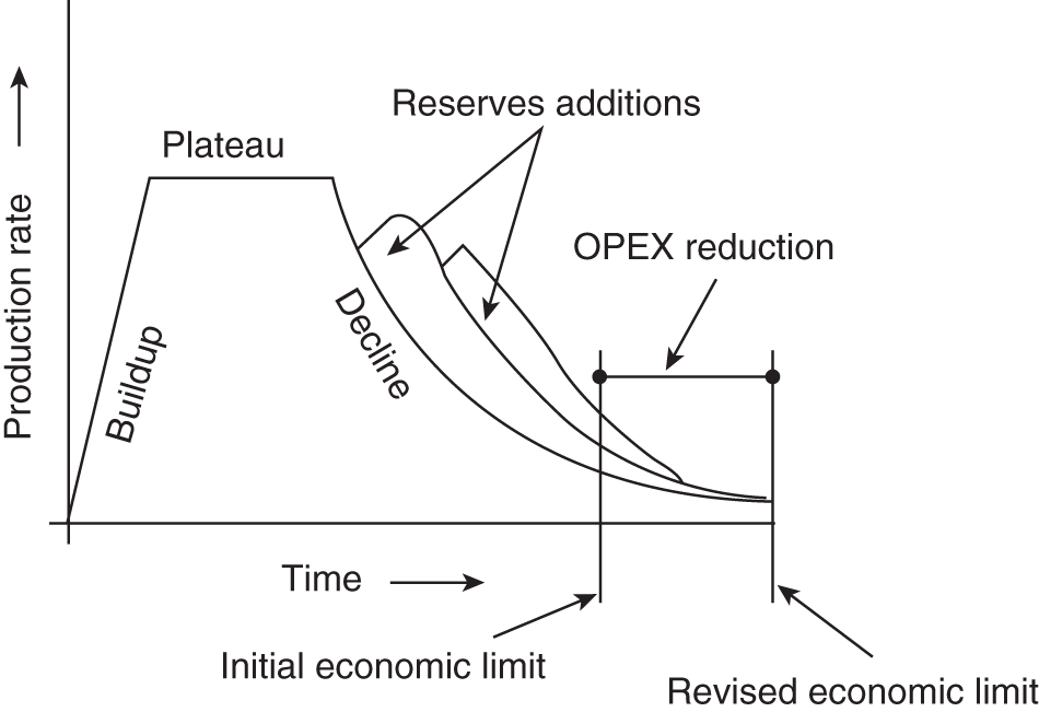
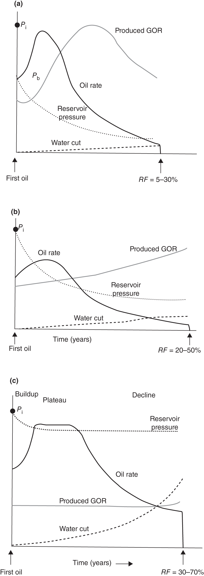
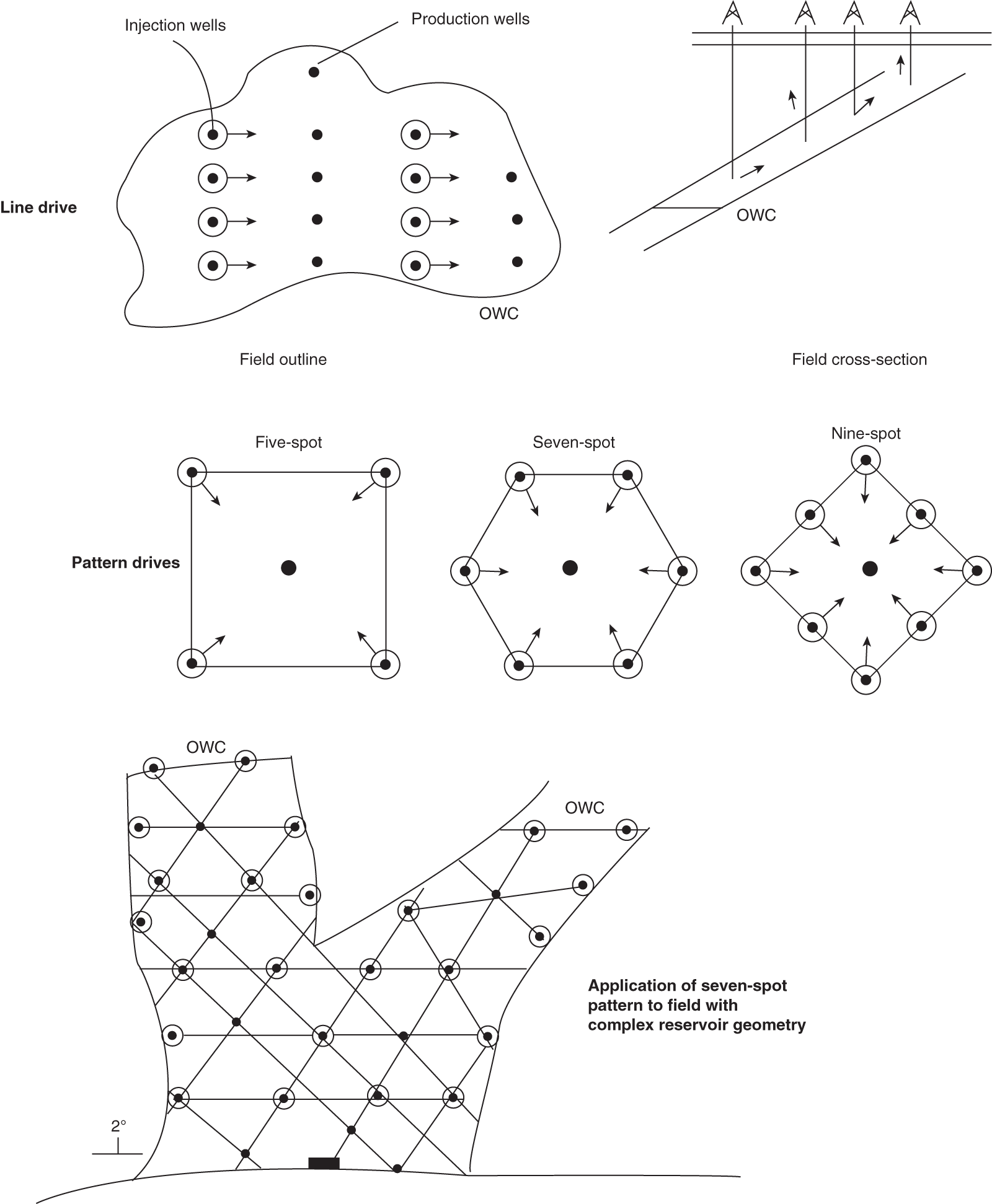
6.2.2 Well Geometries
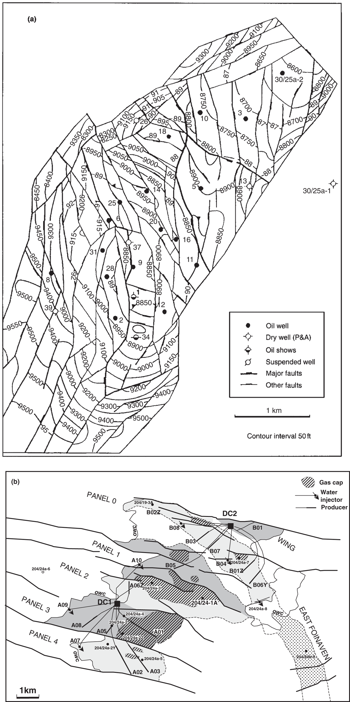
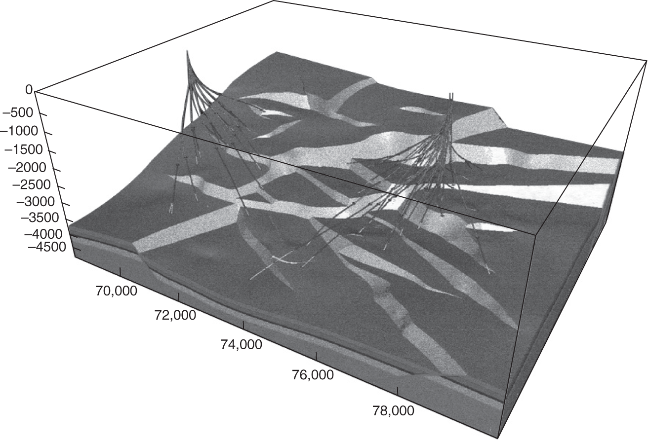
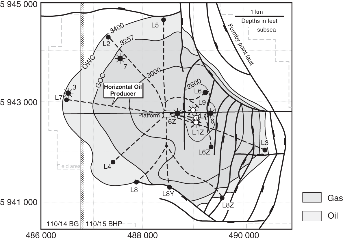
6.2.3 Well Types
6.2.4 Drilling Hazards
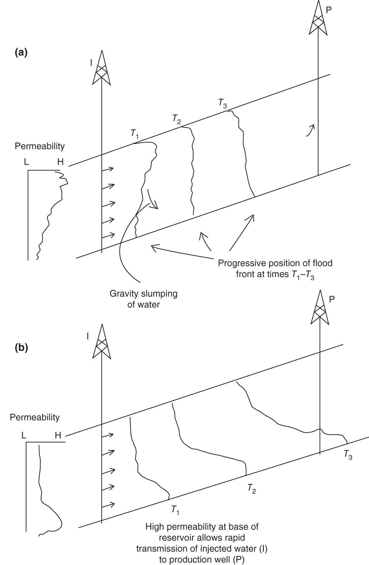
6.2.5 Well Completion and Stimulation
6.2.6 Formation Damage
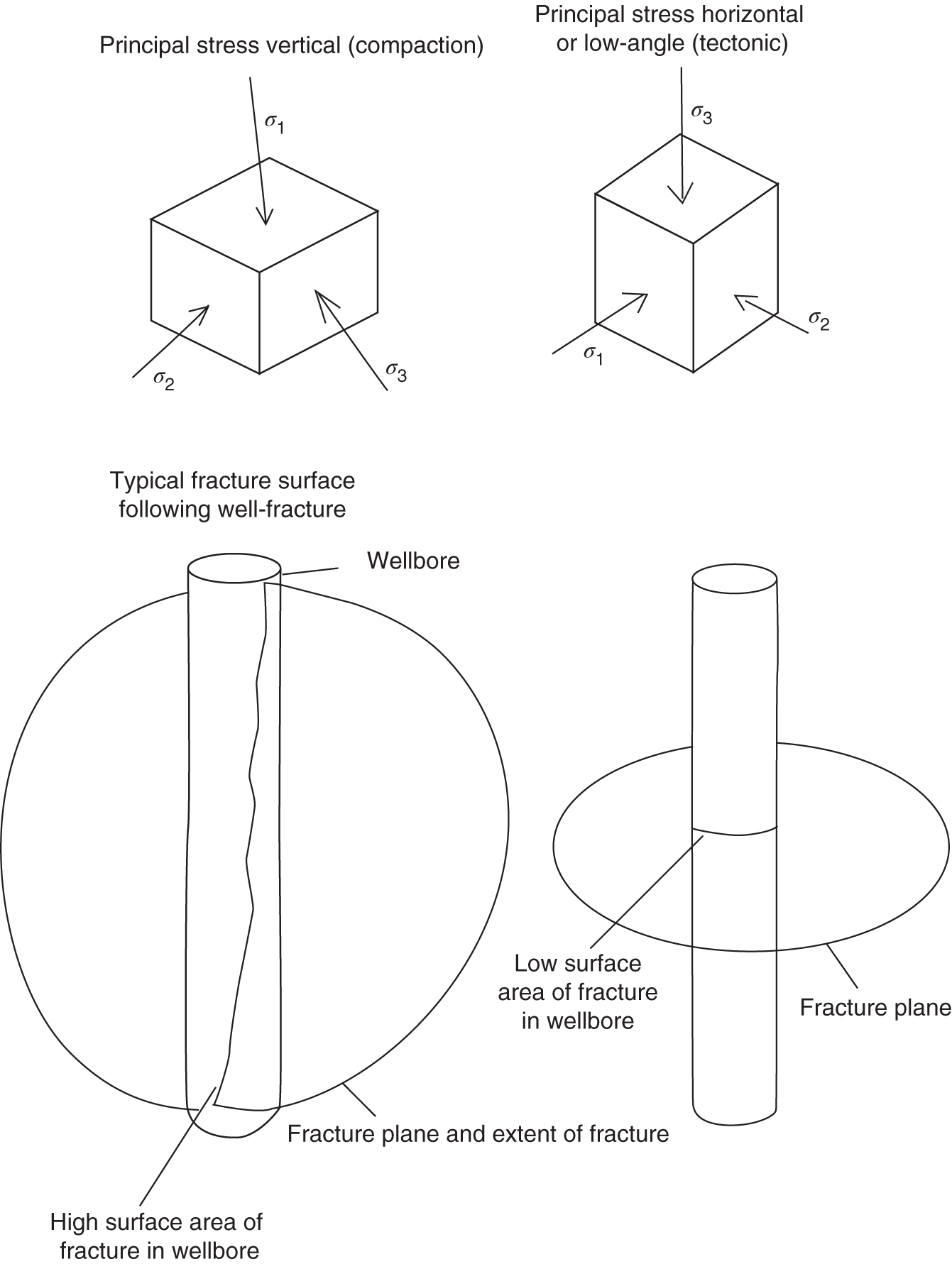
6.2.7 Well Logging and Testing
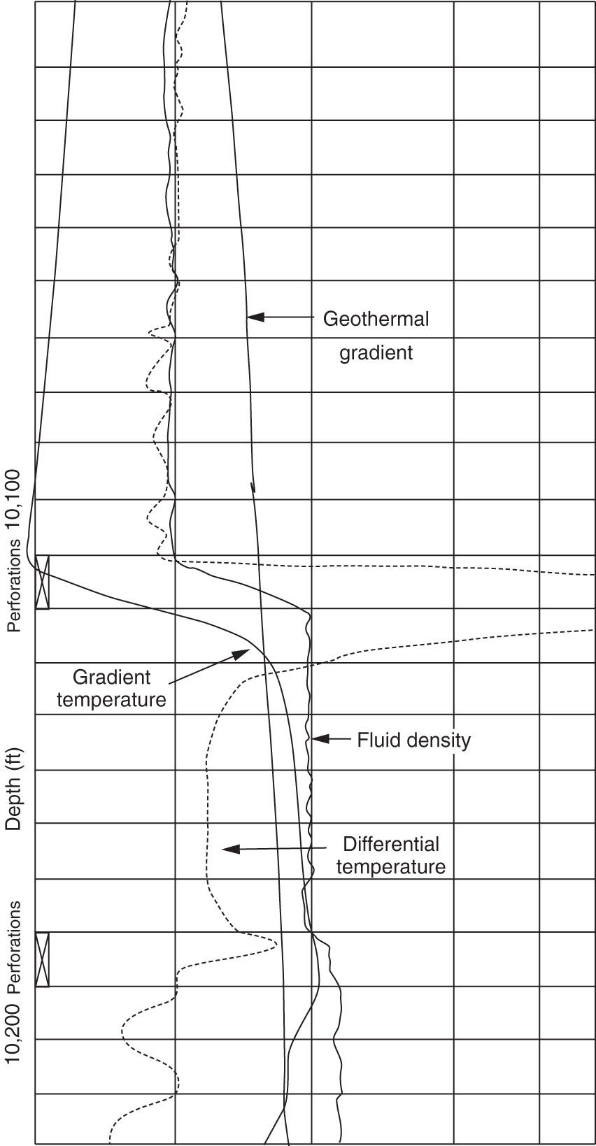
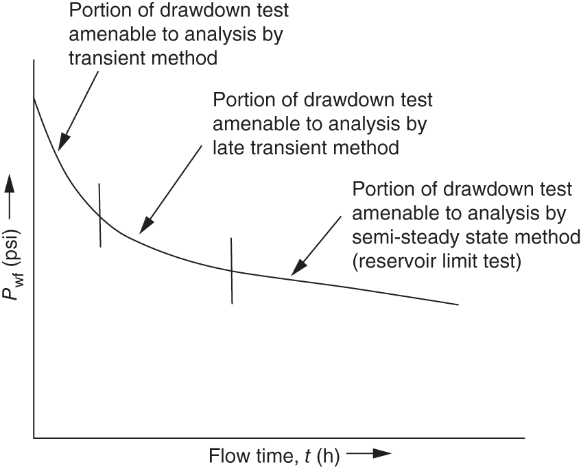
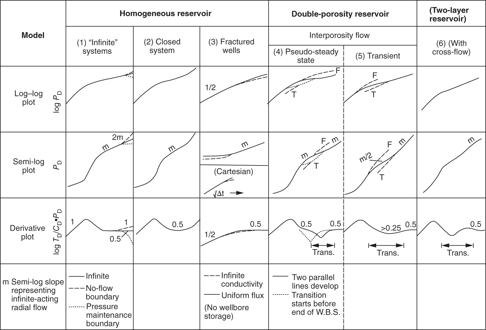
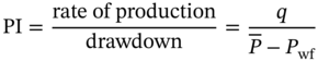
 is the average reservoir pressure; and Pwf is the flowing bottom-hole pressure at the rate q.
6.3 Reservoir Management
6.3.1 Reservoir Description from Production Data
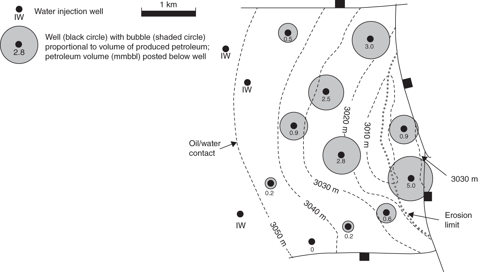
6.3.2 Reservoir Visualization
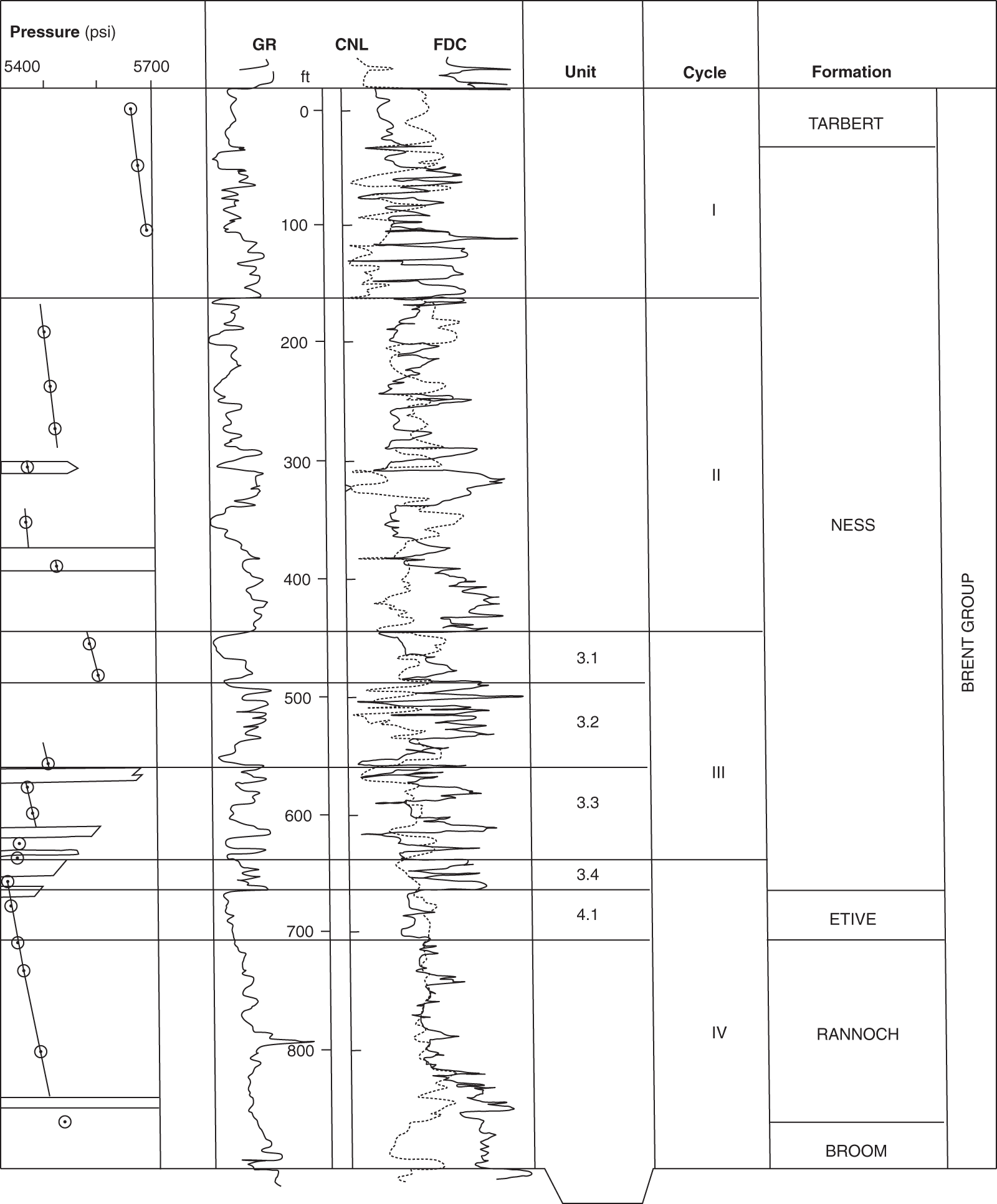
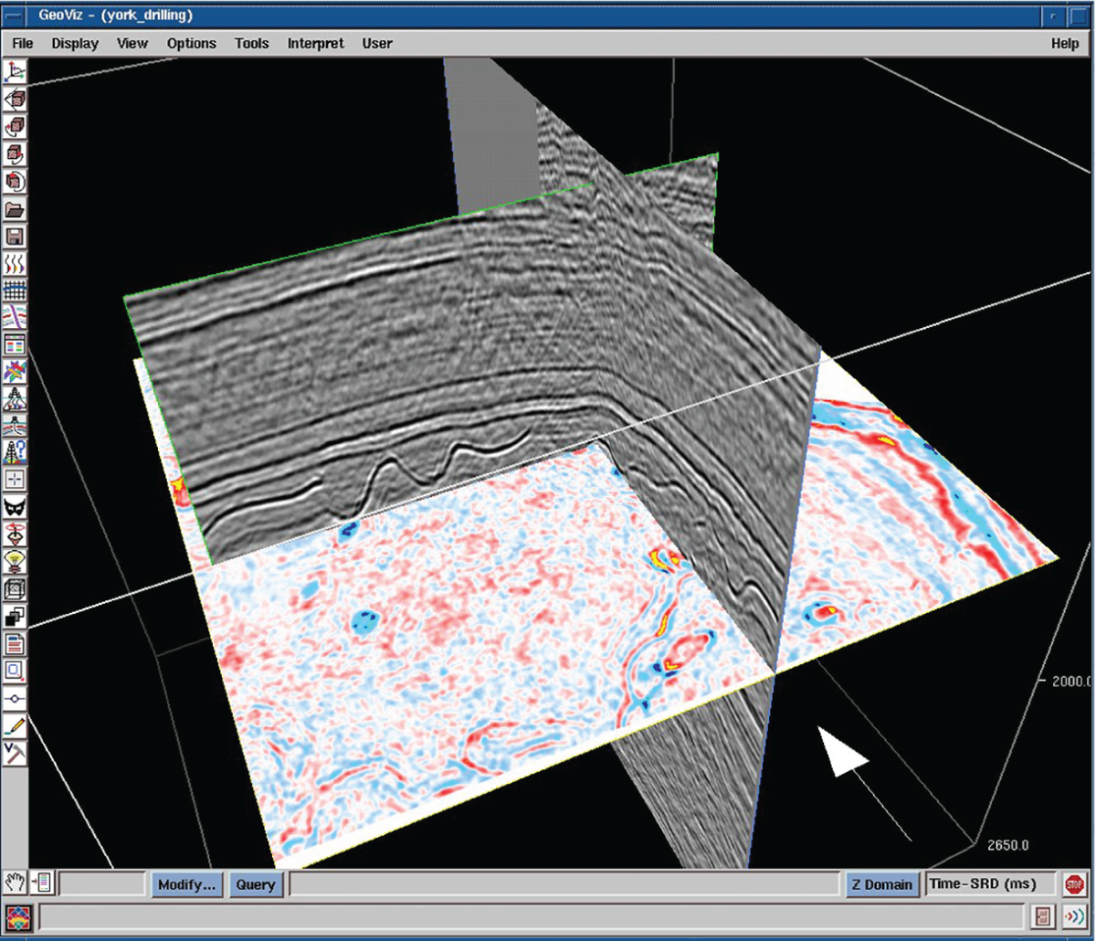
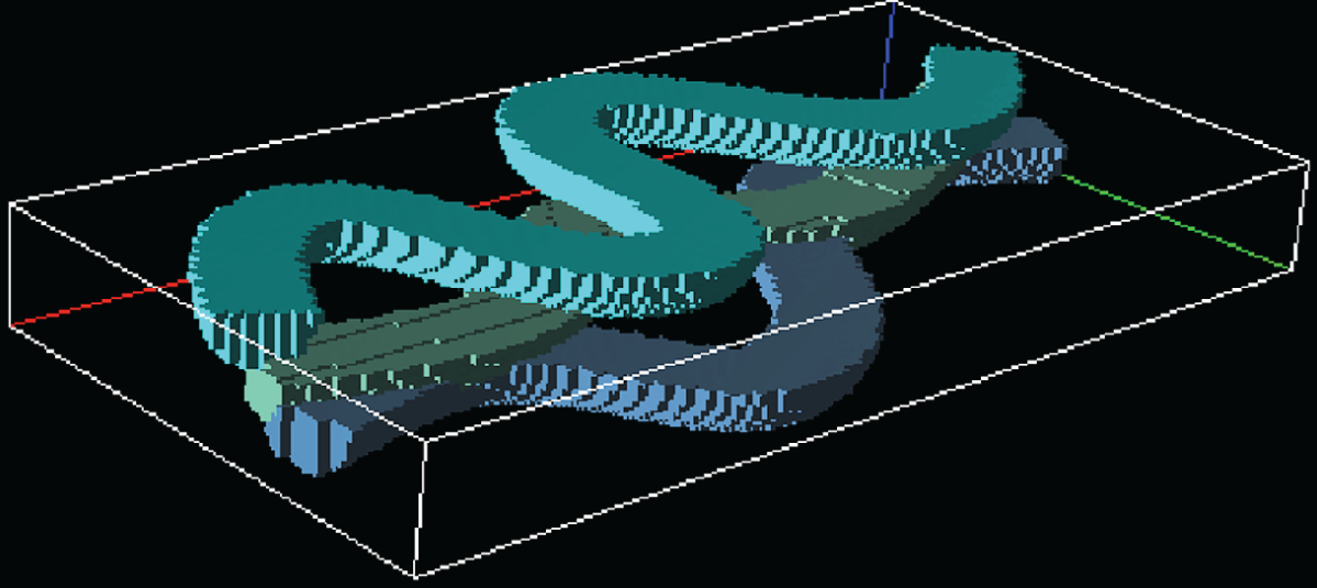

6.3.3 Time-Lapse Seismic
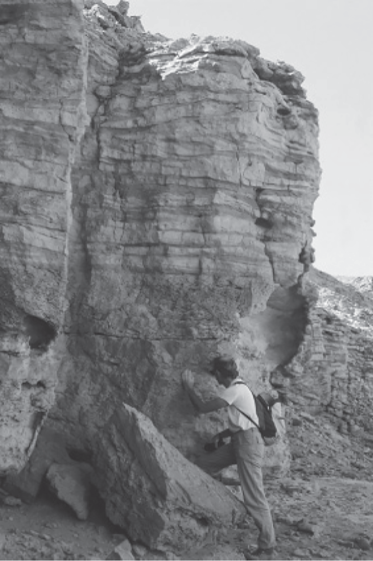
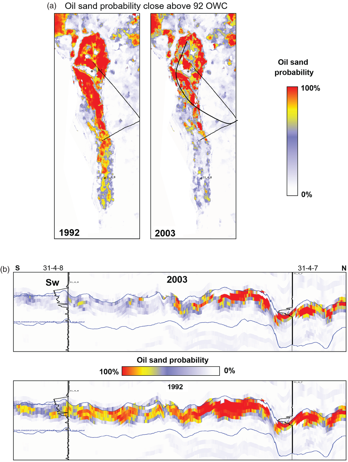
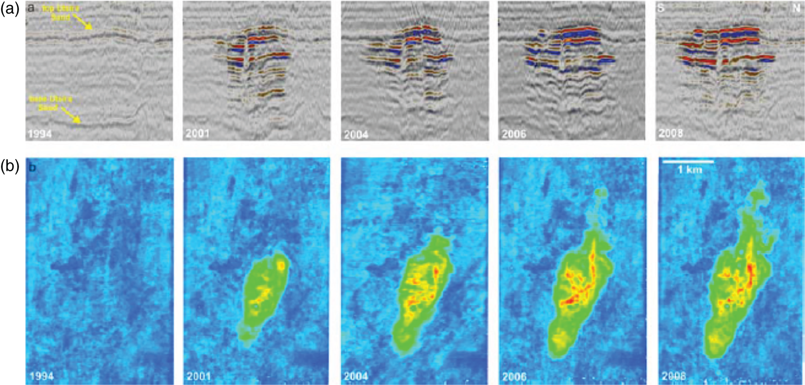
6.3.4 Managing Decline and Abandonment
6.4 Reserves Revisions, Additions, and Field Reactivation
6.4.1 Introduction
6.4.2 Reserves Revisions
6.4.3 Reserves Additions
Well/sand
Activity
Activity cost ($ million)
Expected flow rate (MCF per day)
Gas volume (BCF)
Gas cost ($ per mmscf)
Cash flow ($ thousand per day)
Time to payout (days)
7/G
Perforate
0.5
5–10
5
100
10–20
80
9/G
Perforate
0.1
5
<5
20
10
10
9/F
Perforate
1.5
20
10+
150
40
40
4/E
Sidetrack
5–8
30
15–40
125–530
60
80–130
4/C
Perforate
0.1
10
1
100
20
5
5/E
Perforate
3–4
20–30
1–6
500–4000
40–60
50–100
5/F
Perforate
0.1
10
5–20
20–100
20
5
8/G, D, E
Perforate
5
5–20
5–20
250–1000
10–40
125–500
6/D
Perforate
0.1
5–10
2–5
10–20
10–20
5–10
6/G
Perforate
0.5
5
5
100
10
50
1/F, G, C, D
Perforate
1.0
30
10–20
50–100
60
16
3/G
Perforate
0.5
5
5
100
10
50
3/all
Sidetrack
5–8
25
5–15
300–1600
50
100–160
10/D
Perforate
0.1
5
1–3
33–100
10
10
11/E
New well
8.0
30
30
2.3
60
150
6.4.4 Field Rehabilitation and Reactivation
Case Histories
6.5 Thistle Field, North Sea – Improving Late Field Life Oil Production
6.5.1 Introduction
6.5.2 Field Production Profiles
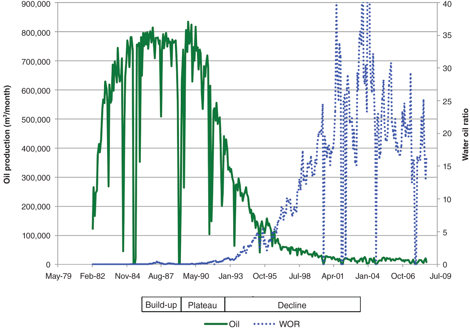
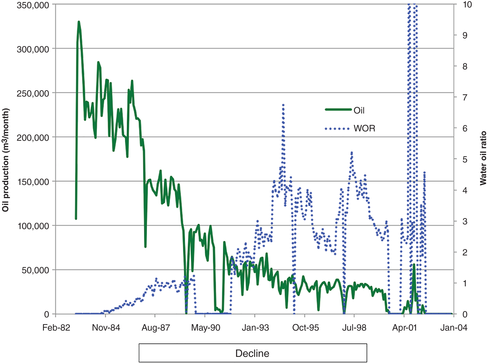
6.5.3 Water Cut and Ultimate Oil Recovery
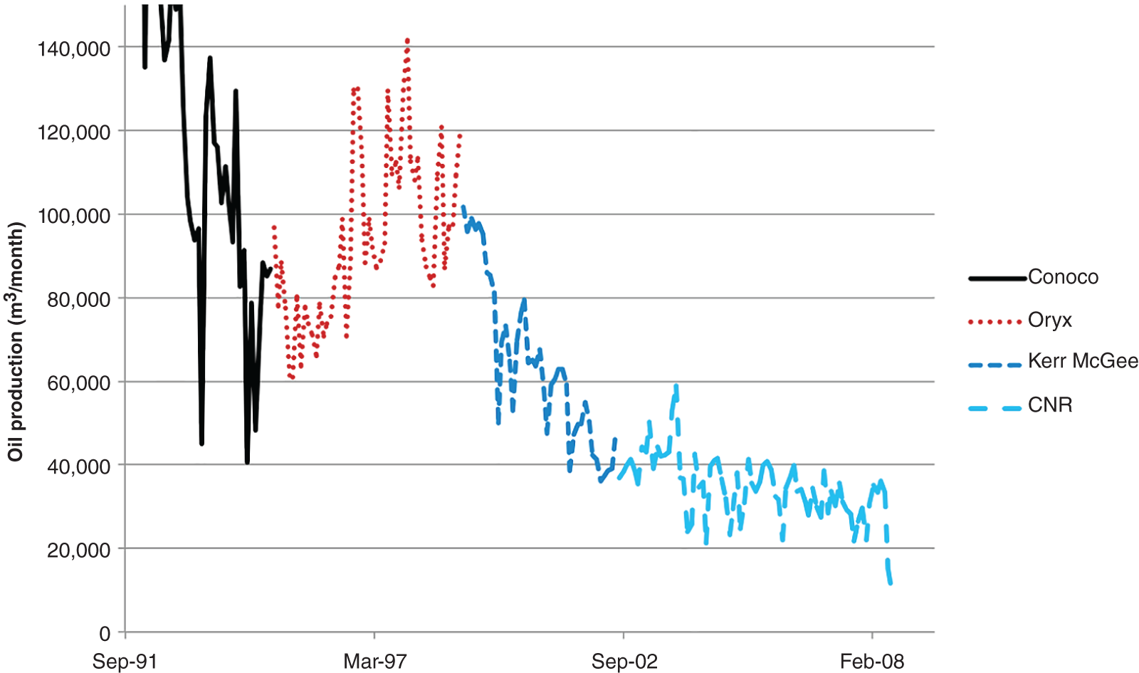
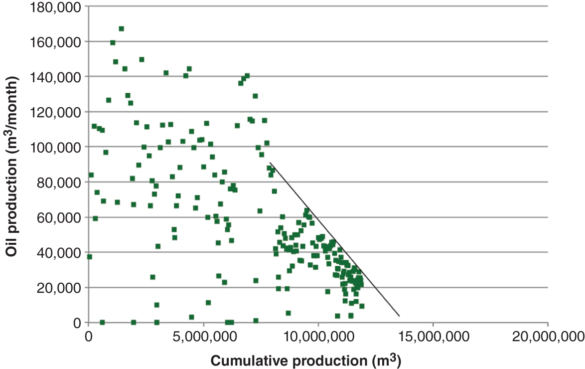
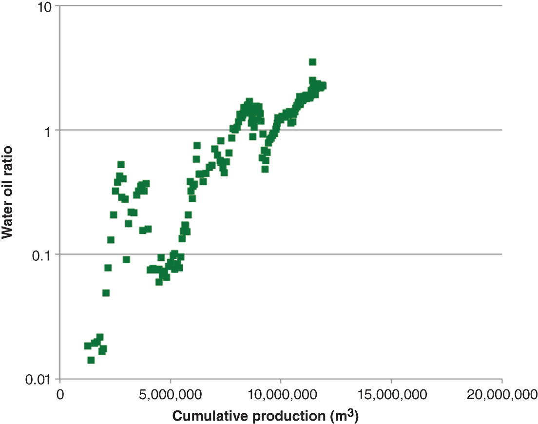
6.5.4 Voidage Replacement, Pressure Maintenance, and Sweep
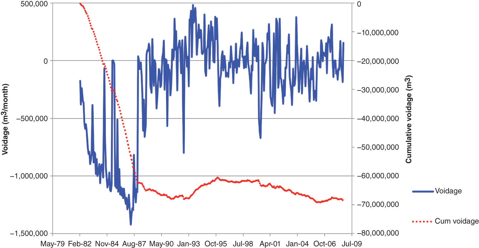
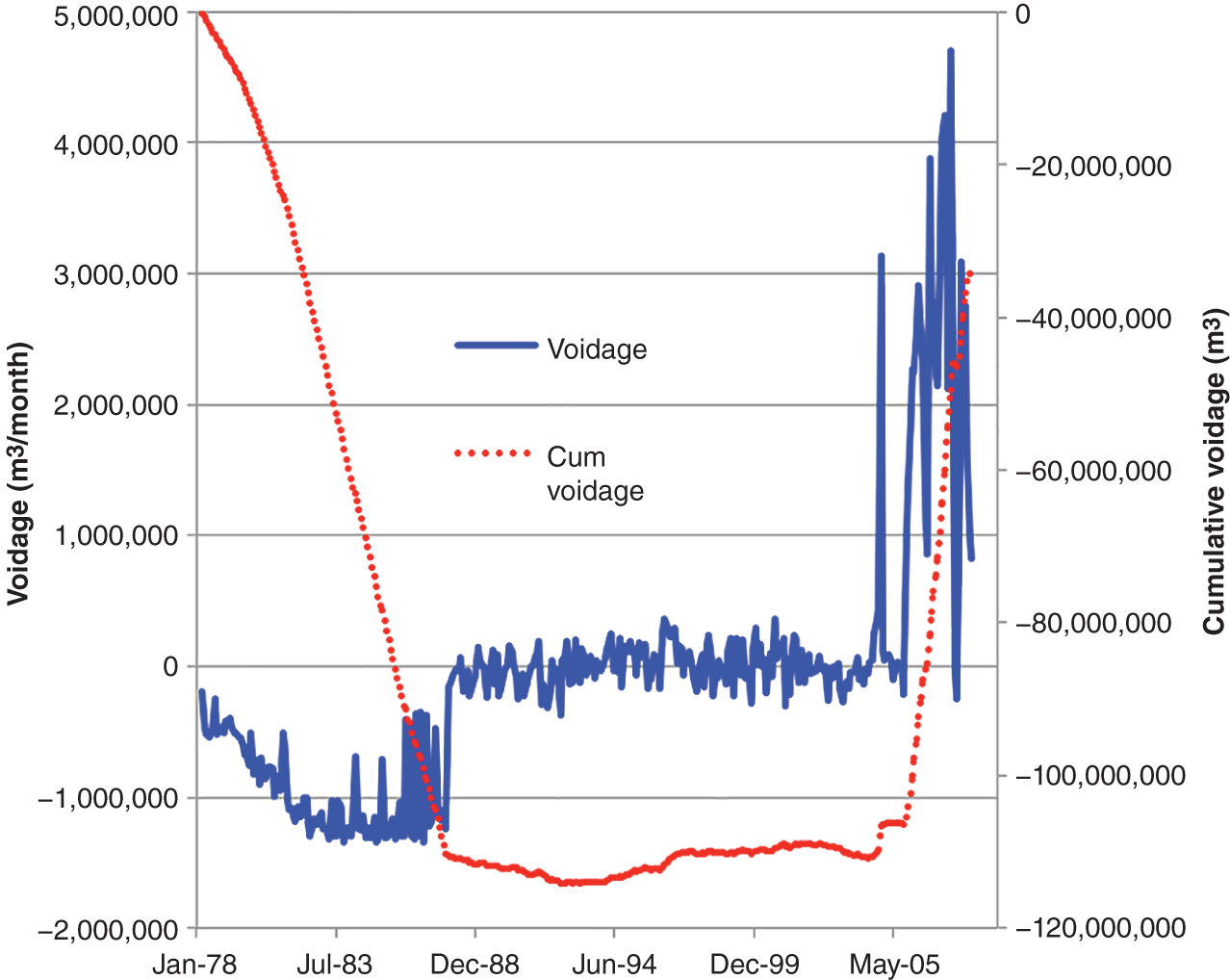
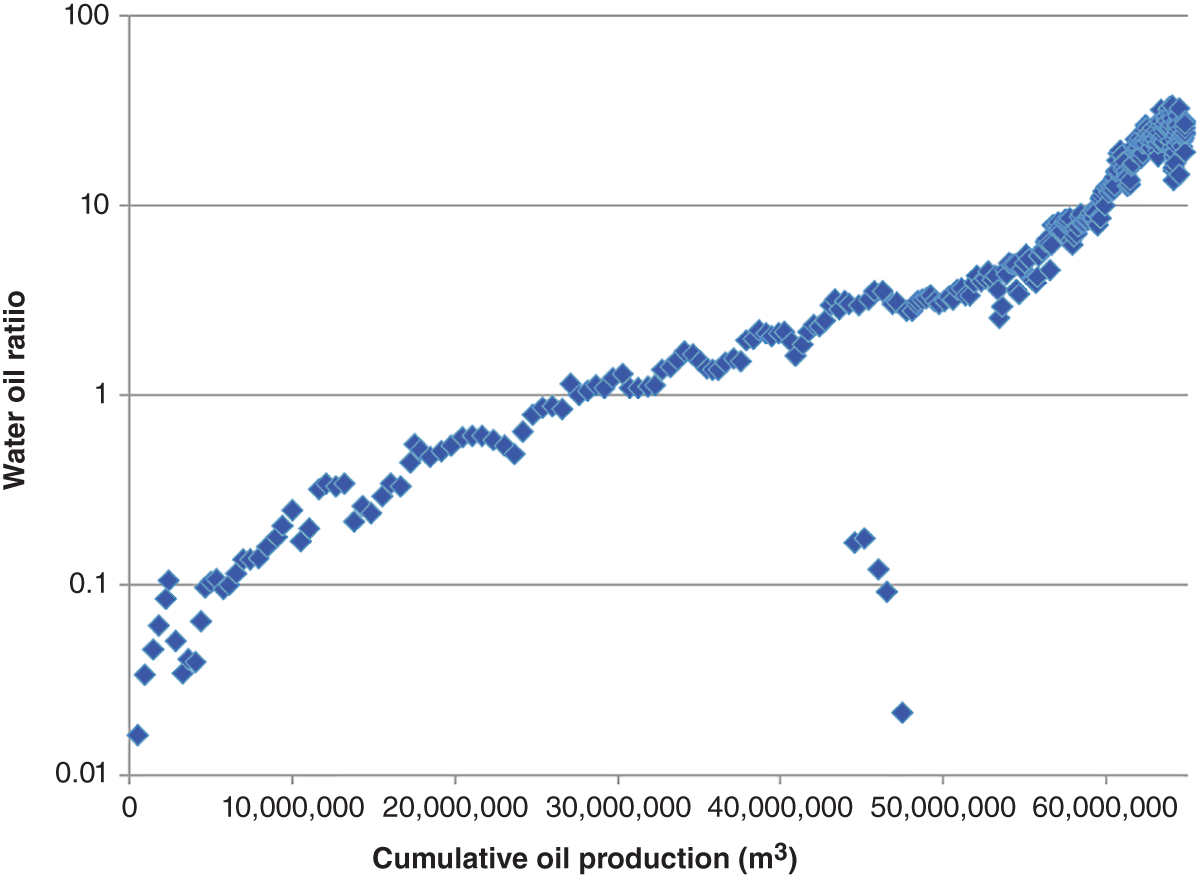
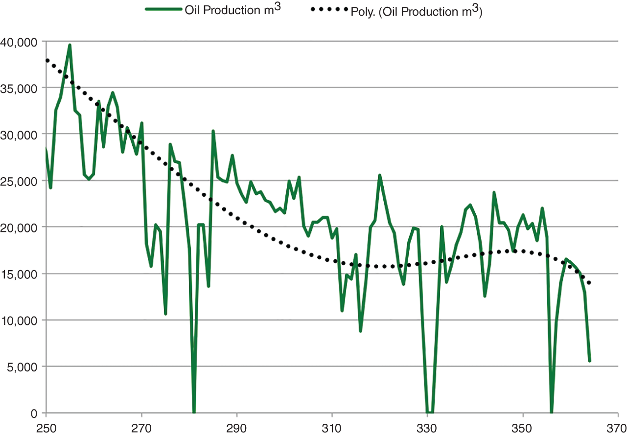
6.5.5 Conclusions
6.6 Ardmore Field, UKCS
6.6.1 Introduction
6.6.2 Location and History
6.6.3 Structure and Stratigraphy
6.6.3.1 Devonian
6.6.3.2 Permian – Rotliegend and Zechstein
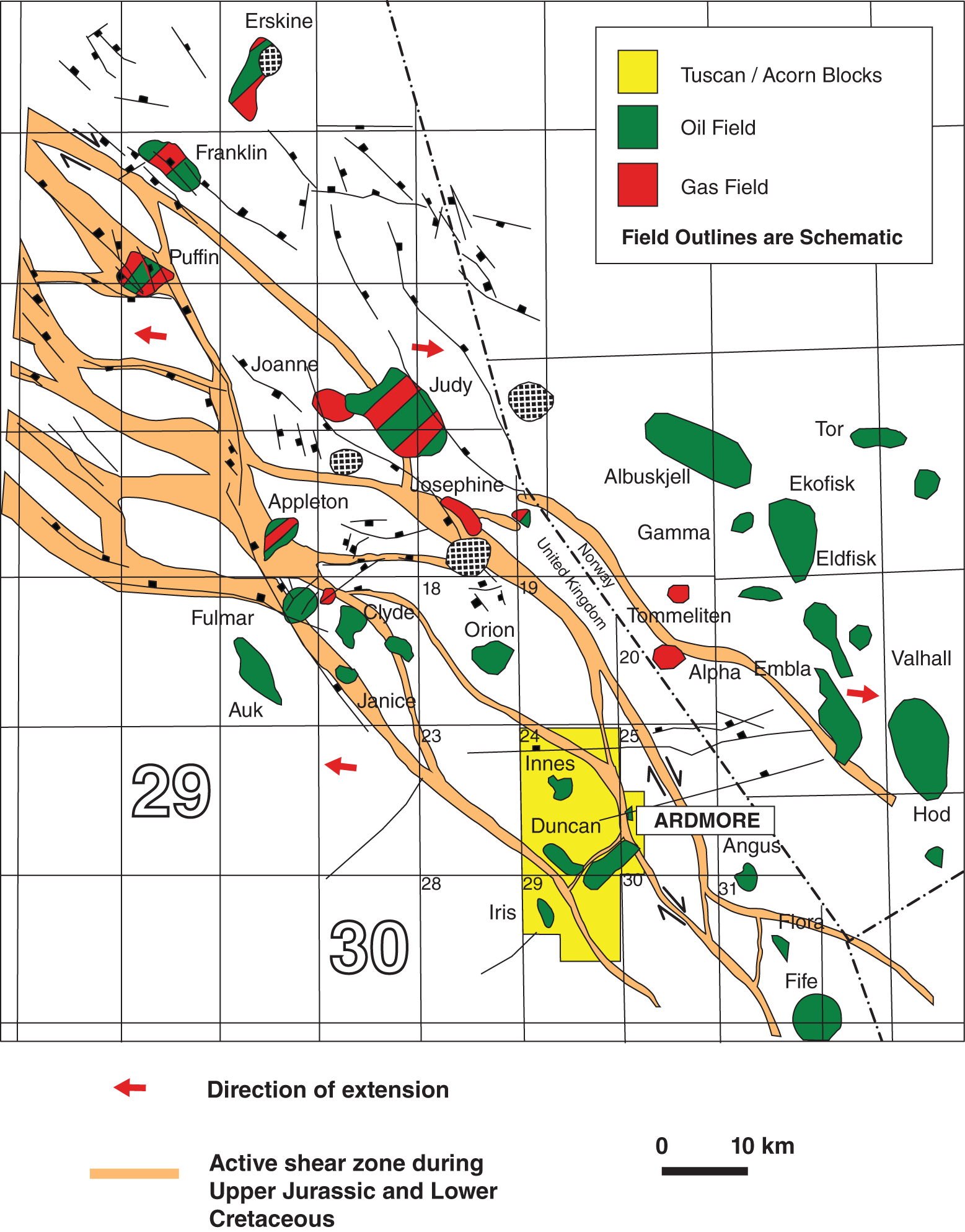
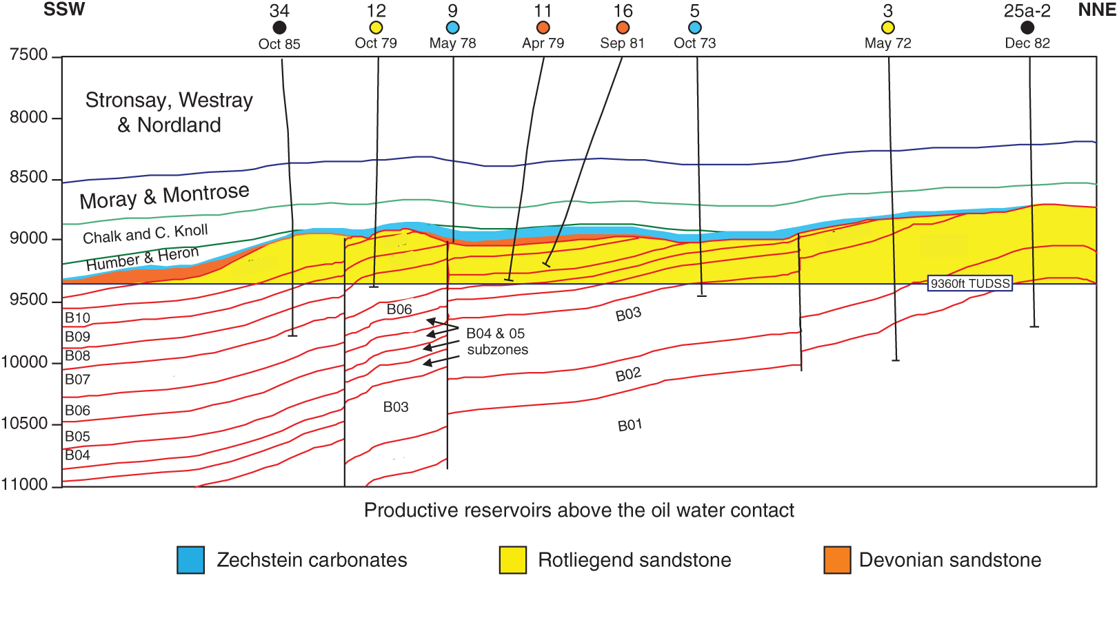
6.6.3.3 Upper Jurassic Humber Group
6.6.3.4 Upper Cretaceous – Paleocene Chalk Group
6.6.3.5 Paleocene/Eocene – Recent Stronsay, Westray, and Nordland Groups
6.6.4 Reservoirs
6.6.4.1 Upper Devonian
6.6.4.2 Rotliegend
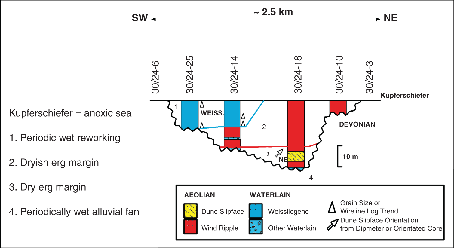
6.6.4.3 Zechstein
6.6.4.4 Upper Jurassic
6.6.5 Source
6.6.6 STOIIP and Reserves
6.6.7 Argyll Production
6.6.8 Ardmore Development and Production
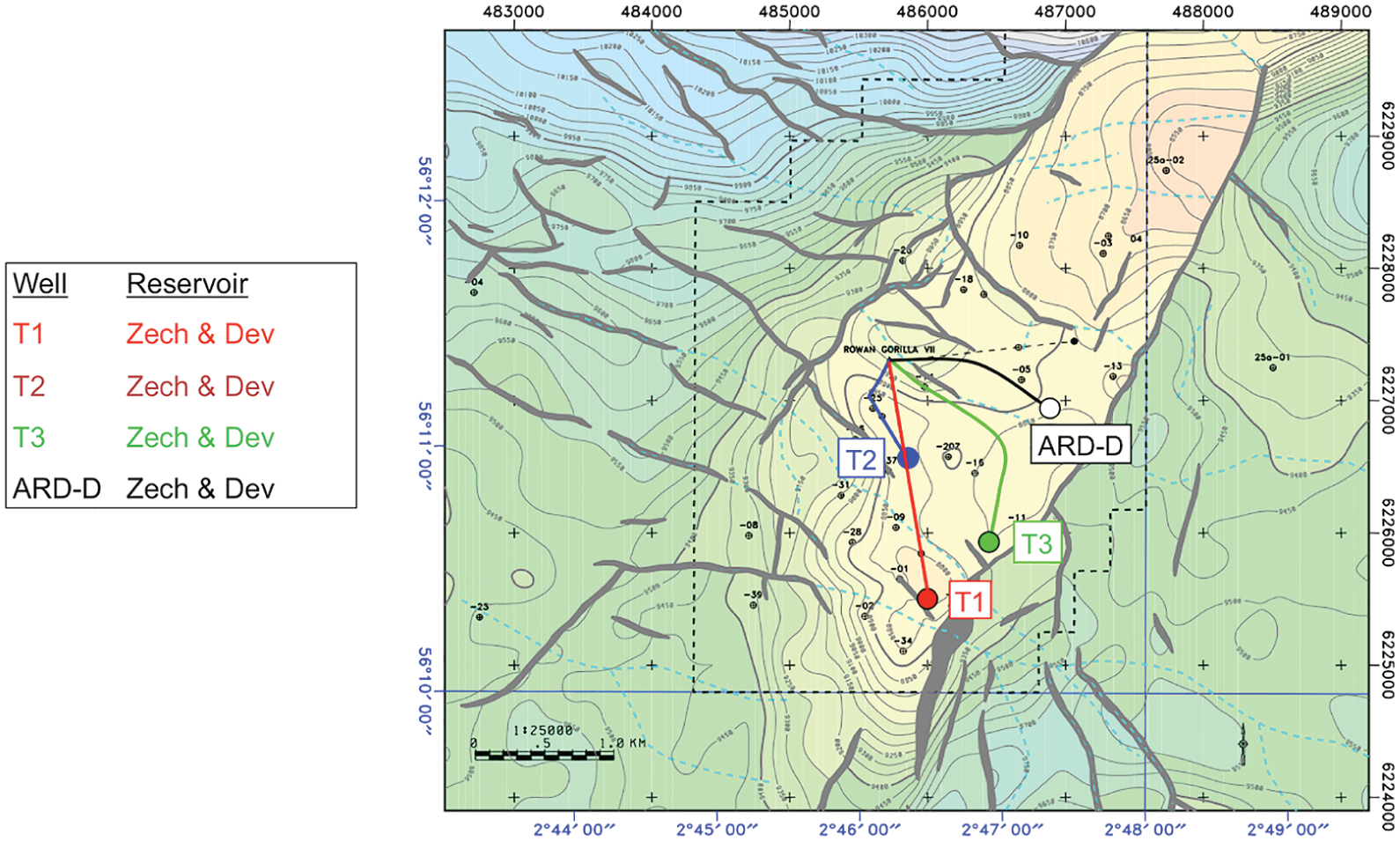

6.6.9 Conclusions
6.6.10 Postscript
Further Reading