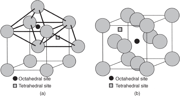
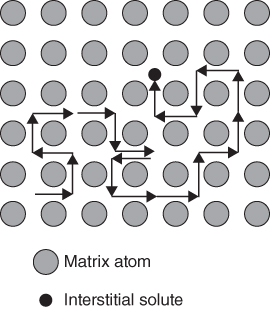
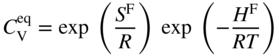
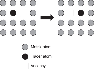
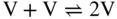
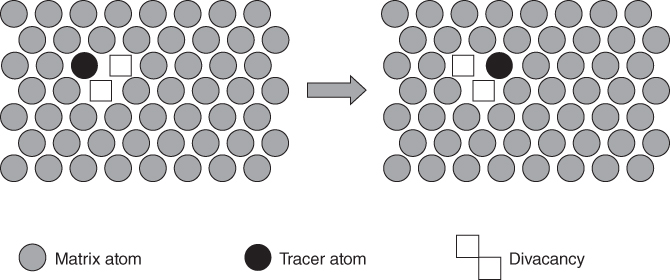
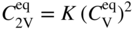
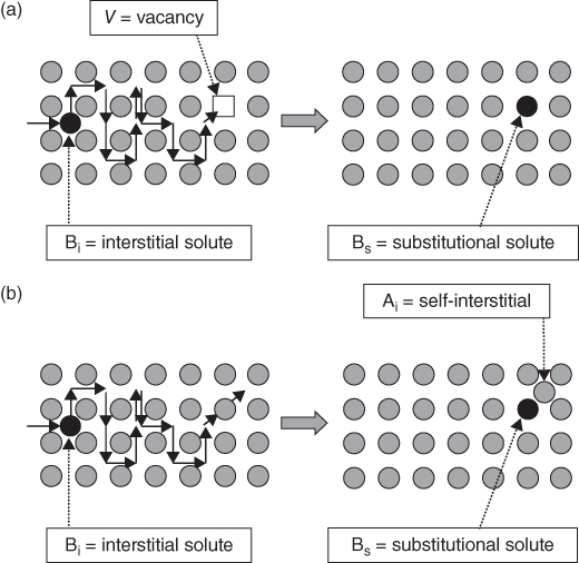
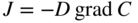
section epub:type=”chapter” role=”doc-chapter”> Diffusion as the process of mitigation and mixing due to irregular movement of particles (atoms, ions, molecules) is one of the basic and ubiquitous phenomena in nature. As this process shows up in all states of matter over very large time and length scales, the subject is still very general involving a large variety of natural sciences such as physics, chemistry, biology, and geology and their interfacial disciplines. Besides its scientific interest, diffusion is of enormous practical relevance for industry and life, ranging from steelmaking, growth of oxide scales, sintering, and high temperature creep of metals to oxide/carbon dioxide exchange in the human lung. It therefore comes as no surprise that the early history of the subject is marked by scientists from diverse communities, e.g. the scottish botanist R. Brown (1773–1858), the scottish chemist T. Graham (1805–1869), the german physiologist A. Fick (1829–1901), the english metallurgist W.C. Roberts‐Austen (1843–1902), and the german physicist A. Einstein (1879–1955). Today, exactly 162 and 112 years after the seminal publications by Fick and Einstein, respectively, the field is flourishing more than ever with more than 10 000 scientific papers per year. The present chapter is confined, of course, to diffusion in condensed matter, namely, in metals, binary alloys, and oxides. Emphasis is on very basic fundamental aspects, the contents being roughly characterized by the headings general theory of diffusion, diffusion coefficients, Matano–Boltzmann analysis, Kirkendall effect, Darken analysis, factors influencing diffusion, impurity diffusion in metals, grain boundary (GB) diffusion in metals, diffusion in solid oxides, morphology of reaction products, and measurement of diffusion parameters. Many references are added at the end of the chapter for readers in the forefront of the subject. Diffusion is defined as “a process whereby particles intermingle as the result of their spontaneous movement caused by thermal agitation.” In the solid state, this manifests itself as the migration of “solute” atoms through a host lattice via the defect structure of that lattice. Since the rate of formation of defects increases with the vibrational energy of the atoms, the diffusion process is enhanced at elevated temperatures. However, the inherently rigid structure of a solid leads to a slow diffusion process as compared with liquids and gases. The basic point defects within a crystal lattice are vacancies and interstitial atoms, and it is via these, and a combination of them, that solid‐state diffusion occurs, in general. Various atomic mechanisms of diffusion in crystals have been identified and are catalogued as follows. Solute atoms that are considerably smaller than the solvent (lattice) atoms (e.g. hydrogen, carbon, nitrogen, and oxygen) are usually incorporated in interstitial sites of a metal. In this way, an interstitial solid solution is formed. Interstitial solutes usually occupy octahedral or tetrahedral sites of the lattice. Octahedral and tetrahedral interstitial sites in the FCC and BCC lattices are illustrated in Figure 5.1. Interstitial solutes can diffuse by jumping from one interstitial site to the next as shown in Figure 5.2. This mechanism is sometimes also denoted as direct interstitial mechanism in order to distinguish it more clearly from the interstitialcy mechanism discussed below. Figure 5.1 Octahedral (a) and tetrahedral (b) interstitial sites in the FCC (left) and BCC (right) lattice. Lattice atoms (open circles); interstitial sites (full circles). Figure 5.2 Direct interstitial mechanism of diffusion. Self‐atoms or substitutional solute atoms migrate by jumping into a neighboring vacant site as illustrated in Figure 5.3. In thermal equilibrium, the atomic fraction of vacancies where SF and HF denote formation entropy and enthalpy of a vacancy (superscript F). Self‐diffusion in metals and alloys and in many ionic crystals (e.g. alkali halides) and ceramic materials occurs by the vacancy mechanism. Figure 5.3 Vacancy mechanism of diffusion. Diffusion of self‐atoms or substitutional solute atoms can also occur via bound pairs of vacancies (denoted as divacancies or as vacancy pairs) as illustrated in Figure 5.4. At thermal equilibrium, divacancies in an elemental crystal are formed from monovacancies according to the reaction Figure 5.4 Divacancy mechanism of diffusion. As a consequence of the law of mass action, we have for the mole fractions CV and C2V of mono‐ and divacancies The quantity K contains the Gibbs free binding energy of the vacancy pair. Since the monovacancy population under equilibrium conditions increases with temperature, the concentration of divacancies In this case, self‐interstitials – extra atoms located between lattice sites – act as diffusion vehicles. As illustrated in Figure 5.5, a self‐interstitial replaces an atom on a substitutional site, which then replaces again a neighboring lattice atom. Self‐interstitials are responsible for diffusion in the silver sublattice of silver halides. In silicon, the base material of microelectronic devices, the interstitialcy mechanism dominates self‐diffusion and plays a prominent role in the diffusion of some solute atoms including important doping elements (Murch and Nowick 1984). This is not surprising since the diamond lattice (coordination number 4) provides sufficient space for interstitial species. Figure 5.5 Interstitialcy mechanism of diffusion. Some solute atoms (B) can be dissolved on interstitial (Bi) and substitutional (Bs) sites of a solvent crystal (A) and diffuse via an interstitial–substitutional exchange mechanism (see Figure 5.6). For some of these so‐called hybrid solutes, the diffusivity of Bi is much higher than the diffusivity of Bs, whereas the opposite is true for the solubilities. Under such conditions, the incorporation of B atoms can occur by the fast diffusion of Bi and the subsequent changeover to Bs. Two types of interstitial–substitutional exchange mechanisms can be distinguished: Figure 5.6 Interstitial–substitutional exchange mechanisms of foreign atom diffusion. (a) Dissociative mechanism. (b) Kickout mechanism. If the changeover involves vacancies (V) according to the mechanism is denoted as dissociative mechanism (sometimes also Frank–Turnbull mechanism or Longini mechanism). The rapid diffusion of Cu in germanium and of some foreign metallic elements in polyvalent metals such as lead, tin, niobium, titanium, and zirconium has been attributed to this mechanism (see Section 5.10). If the changeover involves self‐interstitials (Ai) according to the mechanism is denoted as kickout mechanism. The fast diffusion of Au, Pt, and Zn in silicon has been attributed to this mechanism (Bracht et al. 1995). The considerations above illustrate the main diffusion mechanisms. In the case of semiconducting materials, the simple picture may be complicated to some extent by the wide range of energy values available up to the Fermi level. This range leads to the possibility that the given lattice defect may occur with different states of ionization. However, a useful consequence of this phenomenon is the opportunity to investigate diffusion processes in more detail by using electrical methods. The equation that governs the relationship between the flux J of the diffusing species and the concentration gradient of that species at any point is where D is called the diffusion coefficient of that species. The negative sign indicates a flow from a region of high concentration to that one of lower concentration in an isotropic medium. D may be defined as “the quantity of substance that, in diffusing from one region to another, passes through each unit of cross‐section per unit of time, when the volume‐concentration gradient is unity.” Equation 5.6 is the first Fick’s law. The actual diffusion mechanism, which is operating in a given situation, may be established by the position and the charge state of the diffused impurity, if this information can be obtained. If not, the variation of D in the particular situation may lead to a solution. In particular, the temperature dependence of D is often given by Chitraub et al. (2000) where Q is the activation energy for the jump mechanism while each mechanism has a unique value of Q. Using now the continuity equation for the flow of atoms through a given volume we have with 5.6 which is known as second Fick’s law. For the case of diffusion in one dimension only, this becomes and if D is independent of x, then In order to see which of the above two equations should be applied in any particular case and, further, which boundary conditions must be used in order to find a solution to that equation, it is necessary to consider the possible types of diffusion processes and the ways in which diffusion may be carried out in practical terms. In this case, diffusion occurs in a uniform chemical and defect environment. It is termed self‐diffusion when dealing with solute atoms of the same species as the host lattice and isoconcentration diffusion for the case of foreign atoms. In the latter situation, the crystal must be pre‐diffused to a homogeneous level of impurity concentration prior to the experimental diffusion (Huggins 2001). It is clear that in both cases the solute and solvent atoms must be mutually distinguishable, and this is best achieved by the use of radioisotopes (Section 5.12.3). Under these diffusion conditions, the concentration of the diffusing species is constant, and, consequently, if D is considered to be exclusively a function of C at a given temperature, then D will be independent of position. Therefore, in this case, Eq. 5.11 is always valid. The system is now in a nonequilibrium situation with chemical fluxes being formed by the presence of chemical potential gradients. Diffusion under these conditions is often termed chemical diffusion. Since, in this situation, there exists a concentration gradient ∂C/∂x, Eq. 5.11 is only valid if D is independent of C. Otherwise, one must use the form of Fick’s law shown in Eq. 5.10. However, if it is for the present state assumed that it is valid to use Eq. 5.11, then the boundary conditions, necessary for a solution, are specified by the experimental conditions under which the diffusion is carried out (Vuci and Gladi 1999). In this situation, the total amount of impurity present in the system is small, and the appropriate boundary condition is that the total number of impurity atoms in the diffused region is constant. Experimentally, the impurity is often present as a thin layer, deposited on the surface of the host crystal. The corresponding solution to Fick’s law is where Qi is the number of impurity atoms, per unit area, initially contained in the layer (Labid et al. 1997). Here we have the case in which the number of atoms already diffused into the lattice at any time is small compared with their number available in the source. The appropriate boundary condition is now that the number of impurity atoms per unit volume, C0, at the surface of the crystal is constant for all diffusion times. The corresponding solution is To be more precise, in practice C0 is the solubility of the impurity under the particular conditions of the experiment in question. erfc(y) is a complementary error function given by The most common way of obtaining this condition is to diffuse from a vapor source. This is the method employed for most of the experimental diffusions described in the open literature, and hence the solution shown in Eq. 5.13 is of considerable interest. Provided that the infinite source condition is satisfied, it indicates the theoretical form of the impurity profile for all concentration experiments and those chemical diffusions, where D is independent of C. Any deviation from this profile shape is thus usually an indication that D is a function of C, and Eq. 5.10 must be solved to give the relationship between D and C. The discussion of this problem is presented in a later section. Diffusion in materials is characterized by several diffusion coefficients, which depend on the experimental situation. Our focus is on bulk diffusion in simple binary systems. In this section, we will distinguish the various diffusion coefficients by lower and upper indices. We will drop the indices in the following sections again, whenever it is clear which diffusion coefficient is meant. If the diffusion of A atoms in a solid element A is studied, one speaks of self‐diffusion. Studies of self‐diffusion use a tracer isotope A* of the same element. A typical initial configuration for a tracer self‐diffusion experiment is illustrated in Figure 5.7a. If the applied tracer layer is very thin as compared to the average diffusion length, the tracer self‐diffusion coefficient Figure 5.7 Initial configurations for diffusion experiments: (a) Thin layer of A* on A: tracer diffusion in pure elements. (b) Thin layer of A* or B* on homogeneous alloy: tracer diffusion of alloy components. (c) Thin layer of C* on element A or homogeneous alloy: impurity diffusion. (d) Diffusion couple between metal–hydrogen alloy and a pure metal. (e) Diffusion couple between pure end‐members. (f) Diffusion couple between two homogeneous alloys. The connection between the macroscopically defined tracer self‐diffusion coefficient and the atomistic picture of diffusion is the famous Einstein–Smoluchowski relation. In simple cases, it reads where l denotes the jump length and τ the mean residence time of an atom on a certain site of the crystal. The quantity f is the correlation factor. For self‐diffusion in cubic crystals, f is a numeric factor. Its value is characteristic of the lattice geometry and the diffusion mechanism. In some textbooks, the quantity DE is denoted as the Einstein diffusion coefficient. Equation 5.15 considers only the simplest case: cubic structure, all sites are energetically equivalent, and only jumps to nearest neighbors are allowed. In a homogeneous binary AxB1 − x alloy or compound, two tracer diffusion coefficients for both, A* and B* tracer atoms, can be measured. A typical experimental starting configuration is displayed in Figure 5.7b. We denote the tracer diffusion coefficients by This diffusion asymmetry depends on the crystal structure of the material and on the atomic mechanisms that mediate diffusion. Both diffusivities, of course, also depend on temperature and composition of the alloy or compound and for anisotropic media on the direction of diffusion. When the diffusion of a trace solute C* in a monoatomic solvent A or in a homogeneous binary solvent AxB1 − x (Figure 5.7) is measured, the tracer diffusion coefficients are obtained. These diffusion coefficients are denoted as impurity diffusion coefficients or sometimes also as foreign atom diffusion coefficients. Figure 5.8 shows collected data of self‐diffusion coefficients in sulfides in relation to analogous results obtained for several metal oxides (Mrowec and Przybylski 1984). It becomes clear from this comparison that the rate of self‐diffusion in metal sulfides is generally much higher than in the corresponding oxides. As chemical diffusion coefficients in metal oxides and sulfides are comparable, as shown in Figure 5.9, the significantly higher self‐diffusion rates of cations in the majority of transition metal sulfides result mainly from much higher defect concentration and not their mobilities (see Chapter ). The only known exception is niobium sulfide. Figure 5.8 Comparison of self‐diffusion coefficients in several metal sulfides and oxides. Figure 5.9 Chemical diffusion coefficient in niobium sulfide on the background of analogous data obtained for several metal sulfides and oxides. So far, we have considered in this section cases where the concentration gradient is the only cause for the flow of matter. We have seen that such situations can be studied using tiny amounts of trace elements in an otherwise homogeneous material. However, from a general viewpoint, a diffusion flux is proportional to the gradient of the chemical potential. The chemical potential of a species i in a binary alloy is given by In Eq. 5.16, G denotes Gibbs free energy, ni the number of moles of species i, T the temperature, and p the hydrostatic pressure. The chemical potential depends on the alloy composition. For ideal solutions, the chemical potentials are where Examples of diffusion couples that entail an interdiffusion coefficient are (see Figure 5.7): Interdiffusion results in a composition gradient in the diffusion zone. Interdiffusion profiles are analyzed by the Boltzmann–Matano method or related procedures, as described below. It allows to deduce the concentration dependence of the interdiffusion coefficient from the experimental diffusion profile. As already mentioned, the rate of chemical diffusion and thus the rate of defect mobility in the majority of transition metal sulfides are generally higher than in analogous oxides, but these differences do not exceed 1 order of magnitude (Figure 5.10). Some of the most important results concerning chemical diffusion in transition metal sulfides obtained by Grzesik and Mrowec (2006) are the data describing the mobility of predominant defects in niobium sulfide, being the main product of niobium sulfidation. As it is shown in Figure 5.8, the mobility of these defects is several orders of magnitude lower than that in all other metal sulfides and oxides. It should be noted that one of the most fascinating problems in the case of niobium sulfidation is its extremely high resistance to sulfur attack at high temperatures, in spite of very high concentration of point defects in the growing scale on this metal. The only hypothetical explanation of this unexpected phenomenon was based on the assumption that the mobility of defects in niobium sulfide scale is several orders of magnitude lower than in other transition metal sulfides (Gesmundo et al. 1992). Thus, in spite of a very high concentration of defects, the sulfide scale on niobium shows very good protective properties, comparable with those of the Cr2O3 scale on chromium. Figure 5.10 Comparison of chemical diffusion coefficients in several metal sulfides and oxides. The intrinsic diffusion coefficients (sometimes also component diffusion coefficients) DA and DB of a binary A–B alloy describe the diffusion of the components A and B in relation to the lattice planes. The diffusion rates of A and B atoms are usually not equal. Therefore, in an interdiffusion experiment, a net flux of atoms across any lattice plane exists. The shift of lattice planes with respect to a sample fixed axis is denoted as Kirkendall effect (see Section 5.7). The Kirkendall shift can be observed by incorporating inert markers at the initial interface of a diffusion couple. This shift was observed for the first time for the Cu/Cu–Zn diffusion couples by Smigelskas and Kirkendall (1947). In the following decades, work on many different alloy systems and a variety of markers demonstrated that the Kirkendall effect is a widespread phenomenon of interdiffusion. The intrinsic diffusion coefficients DA and DB of a substitutional binary A–B alloy are related to the interdiffusion coefficient We emphasize that the intrinsic diffusion coefficients and the tracer diffusion coefficients are different. DA and DB pertain to diffusion in a composition gradient, whereas The Matano–Boltzmann analysis is used frequently by researchers to study diffusion in the solid state. By this method, one can measure interdiffusion coefficients, Figure 5.11 (a) Diffusion couple with end‐member compositions where “−” and “+” represent the left‐ and right‐hand end of the reaction couple. Boltzmann (1894) introduced the variable which means that CB is a function of λ only. The relation states that all compositions in a diffusion zone move parabolically in time with respect to one fixed frame of reference. By using the definition of λ, and transforming ∂CB/∂t and ∂CB/∂x in Fick’s second law, using also Eq. 5.20, one can write This treatment is known as the Boltzmann transformation, and this transformation was used for the first time by Matano (1933) to study interdiffusion in the solid state. Initial conditions at time t = 0 can be written as, considering Eq. 5.20, Equation 5.21 contains only total differentials and ∂λ can be canceled from both sides. Integrating from initial composition The data is always measured at some fixed time so that t is constant. If we assume that after annealing the ends of the couple are not affected, then dCB/dx = 0 at and Equation 5.25 defines the plane xM = 0, and the initial contact plane between the end‐members is called Matano plane. The Matano plane position, xM, can be determined from the concentration–penetration curve of the system measured by X‐ray microanalysis by equalizing the areas P and Q as shown in Figure 5.11b. After integrating by parts, Eq. 5.24 can be modified, and, from Figure 5.11c, the interdiffusion coefficient can be expressed in terms of shaded areas as The main disadvantage of this analysis is that one has to find the position of the Matano plane, xM. When the total volume does not change with reaction/mixing, this is easy to determine. However, when the total volume changes, determining the initial contact plane (denoted by x0) is rather confusing. By the Matano–Boltzmann analysis, one can quantify the interdiffusion coefficient, Hartley (1946) was the first to use purposely foreign inert particles, titanium dioxide, in an organic acetone/cellulose acetate system to study the inequality of the diffusing species. Shortly after that, Smigelskas and Kirkendall (1947) used the same technique to examine the inequality of diffusivities of the species in the Cu–Zn system by introducing molybdenum as an inert marker. Researchers dealing with metallic systems at that time were not familiar with Hartley’s work, and the effect of inequality of diffusivities on the inert marker was named the Kirkendall effect (Darken and Gurry 1953). In the experiment by Smigelskas and Kirkendall, a rectangular bar (18 × 1.9 cm2) of 70/30 wrought brass (70 wt%Cu/30 wt%Zn) was taken. This bar was ground and polished, and then 130 µm diameter molybdenum wires, which are inert to the system, were placed on opposite sides of the surfaces. Then a copper layer of 2500 µm was deposited on that, as shown in Figure 5.12. This couple was subjected to annealing at 785 °C. After annealing for a certain time, one small piece was cross‐sectioned to examine, and the rest of the part was further annealed. Following this method, it was possible to get specimens at different annealing times. With annealing, α‐brass grows in between, and after etching, the distance between the markers was measured. If the diffusivities of copper and zinc are the same and there is no change in volume during diffusion/reaction, marker should not move and stay at the original position. Figure 5.12 Schematic representation of a cross section of the diffusion couples prepared by Smigelskas and Kirkendall (1947) before and after annealing at 785 °C. Molybdenum wires moved closer to each other with increasing time, t. However, after measuring, it was clear that with increasing annealing time, the distance between markers decreases parabolically with time. Considering the change in the lattice parameter, it was found that only 1/5 of the displacement occurred because of molar volume change. This shift was explained by Smigelskas and Kirkendall (1947), being possible to draw two conclusions of enormous impact at the time on solid‐state diffusion: Till then, direct exchange or ring mechanisms were accepted as diffusion mechanism in the solid state as shown in Figure 5.13a,b. If any of these mechanisms would be true, then diffusivities of the species should be the same. However, from Kirkendall’s experiment, it is evident that Zn diffuses faster than Cu, which results into the movement of the markers. When zinc diffuses away, all the sites are not occupied by the flow of Cu from opposite direction, and, because of that, vacant sites are left unoccupied. In other sense, there should be a flow of vacancies opposite to the faster diffusing species Zn to compensate for the difference between the Zn and Cu flux. Vacancies will flow toward the brass side, and excess Zn will diffuse toward the Cu side. Ultimately, this results into shrinking in the brass side and swelling in the copper side so that markers move to the brass side. In some diffusion reactions, pores can be found in the product phase. If there is not enough plastic relaxation during the process, vacancies will coalesce to form pores or voids in the reaction layer. Figure 5.13 Atomic diffusion mechanisms: (a) direct exchange mechanism, (b) ring mechanism, and (c) vacancy mechanism. From this experiment, it was clear that diffusion occurs by a vacancy mechanism (Figure 5.13c), and after that the direct exchange and ring mechanisms were abandoned. At first, this work was highly criticized, but later this phenomenon was confirmed from experiments on many other systems (da Silva and Mehl 1951; Nakajima 1997; Sequeira and Amaral 2014). The impact of Kirkendall’s work, at that time, can be realized from Mehl’s comment on his work (Mehl 1947). From Kirkendall’s experiment, it was clear that the diffusion process in solid solutions cannot be described by one diffusion coefficient; rather one has to determine the diffusivity of both species. This was treated mathematically by Darken (1948). Almost at the same time, Hartley and Crank (1949) studied the same subject, and they named the diffusivities of species as intrinsic diffusion coefficient. Seitz (1948) studied the solid‐state diffusion process more extensively. Let us consider a binary diffusion couple of species A and B of the compositions Figure 5.14 Schematic representations of a diffusion couple with the end‐members The intrinsic molar flux at the Kirkendall plane can be expressed by Fick’s first law as This Kirkendall reference plane, xK, is not fixed but moves relative to the laboratory frame of reference. If we consider that this Kirkendall plane moves from xM/0 = 0 with a velocity vK, then the relation between interdiffusion fluxes where In terms of volume flux (volume flux = partial molar volume of component, Vi × molar flux), In an “infinite” diffusion couple (where ends of the couple are not touched by diffusion) from Eq. 5.29, From Eqs. 5.27, 5.30, and 5.31, it follows that By using the standard thermodynamic relations CAVA + CBVB = 1 and VA dCA + VB dCB = 0, Substituting Eq. 5.33 in Eq. 5.28 and comparing with equations CAVA + CBVB = 1 and 5.29 leads to In the special case when partial molar volumes of the components are equal and do not change with the composition so that Vm = VA = VB, Eq. 5.34 reduces to Equation 5.35 is known as the Darken equation. It should be noted that interdiffusion coefficients can be measured at any composition in a concentration profile; however, intrinsic diffusivities can only be measured at compositions indicated by inert markers introduced in the couple prior to annealing. It is well known that diffusion coefficients in solids generally depend rather strongly on temperature, being low at low temperatures but appreciable at high temperatures. Empirically, measurements of diffusion coefficients over a certain temperature range may be often, but by no means always, described by an Arrhenius relation: In Eq. 5.36 D0 is denoted as pre‐exponential factor and ΔH (or Q) as activation enthalpy of diffusion. The pre‐exponential factor can be written as where ΔS is the diffusion entropy and Equation 5.36 is often also written as Eq. 5.7. If the first version of the Arrhenius equation is used, the unit ΔH is kJ mol−1. If the second version is used, the appropriate unit of ΔH is eV per atom. Note that 1 eV per atom = 96.472 kJ mol−1. The gas constant R and the Boltzmann constant kB are related via R = NAkB = 8.314 × 10⁻³ kJ mol−1 K−1, where NA denotes the Avogadro constant. Note that the symbol Q for the activation enthalpy is also widely used in the literature. In an Arrhenius diagram, the logarithm of the diffusivity is plotted versus the reciprocal temperature T−1. For a diffusion process with a temperature‐independent activation enthalpy ΔH, the Arrhenius diagram is a straight line with slope −ΔH/R. From its intercept for T−1 → 0, the pre‐exponential factor D0 can be deduced. Such simple Arrhenius behavior should, however, not be considered to be universal. Departures from it may arise for many reasons, ranging from fundamental aspects of the atomic mechanism, temperature dependence activation parameters, effects associated with impurities, or microstructural features such as GBs. For example, thermodynamics tells us that a temperature‐dependent enthalpy according to automatically entails a temperature‐dependent entropy and vice versa. If enthalpy and entropy increase with temperature, the Arrhenius diagram will show some upward curvature. Nevertheless, Eq. 5.36 provides a very useful standard. The variation of diffusivity with hydrostatic pressure p is far less pronounced than with temperature. Usually, the diffusivity decreases as the pressure is increased. Typical pressure effects range from factors of 2–10 for a pressure of 1 GPa (10 kbar). This variation is largely due to the fact that the Gibbs free energy of activation ΔG varies with pressure according to where ΔV denotes the activation volume and ΔE the activation energy of diffusion. Using Eqs. 5.37 and 5.39, the Arrhenius equation 5.36 can also be written as Thermodynamics tells us that Equation 5.41 can be considered as the definition of the activation volume. Using Eqs. 5.40 and 5.41, the activation volume can be obtained from measurements of the diffusion coefficient at constant temperature as a function of pressure via The term arising from the pressure dependence of We emphasize that a complete characterization of the diffusion process requires knowledge of the three activation parameters ΔH = ΔE + pΔV (valid only for p = const.), ΔS, and ΔV. For solids, the term pΔV becomes significant only at high pressures. At ambient pressure, it is negligible and hence ΔH ≈ ΔE. The various diffusion coefficients in solid systems vary, in general, with the composition of the materials system. However, even in systems where D has a strong concentration dependence, little error is involved in assuming D as a constant, providing that diffusion occurs in a dilute solution or over a small range of concentration. The diffusion in ferritic iron is about 100 times faster than in the austenitic form. This is mainly due to the open BCC structure in the former as compared with a close‐packed FCC structure in the latter. Another effect of crystal structure is the variation of the diffusion coefficient with crystal orientation in a single crystal of the solvent metal. Such anisotropy is nearly or completely absent in cubic metals, but bismuth (rhombohedral space lattice) has a self‐diffusion coefficient about a thousand times larger in the direction parallel to the C‐axis compared with that in a direction perpendicular to it. A significant effect on the diffusion constant has also been noticed if the crystal structure is distorted by plastic strains or by extensive plastic deformation. The strong influences of alloying elements on the hardenability of steels might be the result of factors other than large changes in the rate of diffusion of carbon. That is, impurities usually have a small effect on the diffusion of solute atoms in a solvent metal. In the usual range of grain sizes, it is not necessary to take grain size into account in making diffusion calculations. On the other hand, at lower temperatures, GB diffusion will generally dominate since the bulk or lattice diffusion rate will be small. The arrangement of atoms is different at GBs, near a free surface and adjacent to a dislocation, from that in a regular crystal lattice. As a result, diffusion via vacancy mechanism is greatly enhanced in these regions. Both the number of vacancies and their mobility may be larger as a result of local disruption of crystal regularity. For this reason, activation energy for GB diffusion is less than that of lattice diffusion. In this context, Atkinson et al. (1982) have reported that the oxidation of Ni is controlled by the outward diffusion of Ni ions along GBs in the NiO film at temperatures below 1100 °C. From diffusion results collected for NiO, Atkinson et al. (1986) extracted the boundary diffusivities by assuming a “GB width” of 1 nm. The lattice diffusion coefficient for Ni ions is much larger than that for O ions, as would be expected from the defect structure of NiO. However, the diffusion coefficients for Ni ions in low‐single and high‐single GBs are still larger. The relative contributions to scale growth of bulk and GB diffusion will depend on temperature and oxide grain size. It is generally observed that oxide scales growing on metals have rather fine grain sizes (on the order of a micrometer) so boundary diffusion can predominate to quite high temperatures. It is reported for NiO that boundary diffusion has a similar oxygen pressure dependence to bulk diffusion, which suggests that similar point defects control both processes. In summary, the diffusion coefficient is a function of many variables, such as temperature, pressure, concentration, crystal structure, impurities, grain size, and short circuit along the GBs, dislocations, or surfaces, but also of an electric field or a local state of stress. Let us now consider a very dilute substitutional binary alloy of metals A and B with the mole fraction of B atoms much smaller than that of A atoms. Then A is denoted as solvent (or matrix), and B is denoted as solute. Diffusion in a dilute alloy has always two aspects: solute diffusion and solvent diffusion. In this section we consider only solute diffusion in very dilute FCC alloys. This is often denoted as impurity diffusion. It implies that the solute is isolated from other solutes in the matrix. In what follows, we consider only fast solute diffusion in some polyvalent metals, which are sometimes also denoted as open metals (Wenwer et al. 1989). Open refers to the large ratio between atomic and ionic radius of the solvent. This solvent property leads to solutes with relatively small radii to the occurrence of fast solute diffusion. Fast solute diffusion in metals has been attributed to the dissociative mechanism (Nowick and Burton 1975). This mechanism operates for solutes that are incorporated not only on substitutional sites but also to some extent to interstitial sites of the solvent metal. As discussed above, the dissociative reaction involves vacancies. Provided that local equilibrium is established, the concentrations of the three involved species must fulfill the law of mass action: where Ci, Cs, and CV denote molar fractions of interstitial solute, substitutional solute, and vacancies, K(T) is a constant that depends on temperature, and the superscript eq denotes thermal equilibrium. A metal crystal with a normal density of dislocations has a sufficient abundance of vacancy sources or sinks to keep the vacancies everywhere at equilibrium. Then, the effective diffusivity of solutes is given by Murch and Nowick (1984): where Di denotes the diffusivity of the solute in its interstitial state and Ds its vacancy‐mediated diffusivity on substitutional sites. For solutes with dominating interstitial solubility and diffusivity ( For so‐called hybrid solutes, the substitutional solubility dominates ( This relation contains the factor where Gis denotes the Gibbs free energy difference between the interstitial and substitutional positions of the solute. The rather wide diffusivity dispersion of fast solute diffusers can be largely attributed to this factor. Fast diffusion of solutes is well known for the semiconducting elements silicon and germanium (Seeger and Chik 1968). It has been also attributed to interstitial–substitutional exchange mechanisms. The kickout mechanism is dominating diffusion of Au, Pt, and Zn in silicon (Bracht et al. 1995), whereas the dissociative mechanism is operating, e.g. for Cu and germanium (Franck and Turnbull 1956). From a chemical viewpoint, these similarities are not surprising. Silicon and germanium are group IV elements such as the “open” metals lead and tin. Fast diffusion is also observed for compound semiconductors (e.g. Zn in GaAs [Stolwijk et al. 2001]). Actually, the concepts growing out from studies of fast diffusion in semiconductors have strongly influenced the interpretation of fast diffusion in metals (Murtagh et al. 2001). GB diffusion plays an important role in many processes taking place in engineering materials at elevated temperatures. Such processes include Coble creep, sintering, diffusion‐induced GB migration, discontinuous reactions (such as discontinuous precipitation, discontinuous coarsening, etc.), recrystallization, and grain growth. The fact that GBs provide high‐diffusivity (“short‐circuit”) paths in metals has been known since a few decades. First indications of enhanced atomic mobility at GBs were obtained as early as in the 1920–1930s, for example, from grain size dependence of creep and sintering rates in polycrystalline materials. However, the first direct proof of GB diffusion was obtained in the early 1950s using autoradiography: the additional blackening of autoradiographic images along GBs indicated that the radiotracer atoms penetrated into GBs much faster than in the regular lattice. These observations were immediately followed by two important events: the appearance of the nowadays classic Fisher model of boundary diffusion, on one hand, and the development and extensive use of the radiotracer serial sectioning technique, on the other hand. It was largely due to these events that GB diffusion studies were put on a quantitative basis and GB diffusion measurements became the subject of many investigations and publications (Kaur et al. 1989, 1995). This section presents a brief review of fundamentals of GB diffusion on metals and metallic alloys. Most mathematical treatments of GB diffusion are based on the Fisher model (1951) describing diffusion along a single GB. In the Fisher model, a GB is represented as a high‐diffusivity uniform and isotropic slab embedded in a low‐diffusivity isotropic crystal perpendicular to its surface (Figure 5.15). The GB is thus described by two physical parameters: the GB width δ and the GB diffusion coefficient Db such that Db > D, D being the volume diffusion coefficient. In a typical diffusion experiment, a layer of foreign atoms, or tracer atoms of the same material, is created at the surface, and the specimen is annealed at a constant temperature T for a time t. During the anneal, the atoms diffuse from the surface into the specimen in two ways: directly into the grains and, much faster, along the GB. In turn, the atoms that diffuse along the GB eventually leave it and continue to diffuse in the lattice regions adjacent to the GB, thus giving rise to a volume diffusion field around the GB. Figure 5.15 Schematic geometry of the Fisher model of grain boundary diffusion. Mathematically, the diffusion process is described by two coupled equations: These equations represent diffusion in the volume and along the GB, respectively. C(x,y,t) is the volume concentration of the diffusing atoms, and Cb(y,t) is their concentration in the GB. The second term in the right‐hand side of 5.49 takes into account the leakage of the diffusing atoms from the GB to the volume. Any solution of 5.48 and 5.49 should meet the surface condition, which can be different in different experiments (see below), as well as the natural initial and boundary conditions at x → ±∞ and y → ∞. The joining condition between functions C(x,y,t) and Cb(y,t) depends on whether we study self‐diffusion of impurity diffusion. For self‐diffusion, the joining condition simply reflects the continuity of the concentration across the GB: For impurity diffusion, the joining condition involves the equilibrium segregation factor s and reads where s is the segregation factor. The determination of the triple product sδDb of impurity diffusion is relatively easy if s is constant. In the case of self‐diffusion, we can only determine the product δDb. We thus need to know δ if we want to determine the GB diffusion coefficient Db. The assumption δ = 0.5 nm introduced by Fisher (1951) seems to be a good approximation. This value of δ is well consistent with evaluations of GB width by high‐resolution transmission electron microscopy, field ion microscopy, and other techniques (Howe 1997; Kaur et al. 1995). Furthermore, recent combined B‐regime and C‐regime measurements of self‐diffusion in silver indicate that δ = 0.5 nm is a very good estimate of δ in metals. Atomistic computer simulations also confirm that the enhanced diffusivity at GBs is confined to the GB core of around 0.5 nm in thickness (Keblinski and Yamakov 2003; Suzuki and Mishin 2003). It should be noted that type B kinetics is the regime in which where d is the spacing between the GBs. In this type, GB diffusion is accompanied by volume diffusion around GBs, but volume diffusion fields of neighboring GBs do not overlap. If, starting from the B regime, we go toward lower temperatures and/or shorter anneal times, we eventually arrive at a situation when volume diffusion is almost “frozen out” and diffusion takes place only along GBs without any leakage to the volume. In this regime, called type C, we have and then the concentration profile is either a Gaussian function (instantaneous source) or an error function (constant source) Atomistic computer simulations (Sörensen et al. 2000; Suzuki and Mishin 2003) suggest that the full description of GB diffusion should include both the vacancy and interstitial‐related mechanisms. Simulations also reveal that vacancies can move by “long jumps” involving a simultaneous displacement of two or more atoms. Interstitials move by the interstitialcy mechanism in which two or more atoms jump in a concerted manner. On some (although rare) occasions, even the ring mechanism was found to operate in certain GBs (Sörensen et al. 2000). Which mechanism dominates the overall atomic transport depends on the particular GB structure. Atomistic modeling also suggests that at high temperatures, GBs can develop a significantly disordered, “liquid‐like” structure (Keblinski et al. 1999). Diffusion in such GBs is believed to occur by mechanisms similar to those in liquids. Many technologically important kinetic processes occurring in systems containing oxides are dependent on the mobility of atoms and ions through the oxide phases. In order to determine the rate and the atomic mechanisms by which processes such as sintering, oxidation, creep, grain growth, and various solid‐state reactions occur, it is essential to determine the nature and the rate of diffusion of the several species contributing to the process of interest. In general, diffusion‐controlled processes, such as the oxidation of metals, occur, not in homogeneous oxides, but under conditions where a chemical potential gradient exists. These gradients may result from the oxide being in contact with several different oxygen potentials, thermal energy sources, or phases of varying chemical composition. In such cases, the process is controlled by chemical diffusion, which takes into account the existing chemical potential gradient, rather than by self‐diffusion. A number of investigations have been conducted, therefore, with the goal of measuring chemical diffusion in oxides. In addition, a number of equations have been developed to relate self‐diffusion to chemical diffusion. Many of these aspects are treated in sections above, in this chapter. Moreover, in Chapter , the nature of the point defects in oxides is described, and examples of the relationships that exist among these imperfections are presented. The influence of stoichiometry and foreign atom concentration on the point defect disorder is also emphasized. In general, diffusion mechanisms are discussed, the various kinds of diffusion coefficients are defined, the main equations relating these diffusivities are presented, etc., but many subjects are omitted because there is a great diversity of information that has been obtained from diffusion studies. Being impossible to be further comprehensive, here we will turn to a brief overview of diffusion in oxides, and then more attention will be placed on the influence of external forces on the diffusion in oxides. Studies of cation self‐diffusion in oxides have been most fruitful when directed toward those compounds that have homogeneity regions greater than about 0.01%. In these cases, it has been possible to measure intrinsic diffusivities as a function of oxygen pressure under conditions where impurity levels were low. By comparing results obtained from studies with “pure” intrinsic crystals with those for specimens doped with aliovalent foreign atoms, it has been possible not only to establish the nature of the type and charge of the atomic point defects controlling diffusion but also to separate the enthalpies and entropies of defect formation and migration. In addition, diffusion studies, together with measurements of other defect structure‐dependent properties, have revealed the complex nature of atomic disorder that occurs in many oxides. In some cases, a satisfactory interpretation of experimental results requires the invocation of defect models that include the existence of defects with several different charge levels as VCo′, Attention has been directed toward understanding the atomic defect structures of oxides with very narrow homogeneity ranges, such as Al2O3. For these cases, careful studies with known aliovalent foreign atom additions can be employed to establish the nature of the diffusion mechanisms for such impurity‐sensitive compounds. Conversely, it is clear that large discrepancies in diffusivities obtained by different investigators can often be traced to differences in purity of specimens used in the various studies. It is apparent that the results of some early studies of oxygen diffusion in oxides may be in error because of the many difficulties involved in the use of the 16O–18O exchange method. Nevertheless, diffusion data obtained in recent years has been the single most important source of information available for the development of our understanding of the oxygen sublattice defect structure. This is particularly true for the oxygen‐excess p‐type conductors for which the primary disorder is on the cation sublattice. Available evidence shows that both oxygen vacancies and oxygen interstitials exist in appreciable concentrations in different oxides. From studies on compounds such as CoO and CdO, it has been further established that the defects on the oxygen sublattice are charged and that their concentrations may be influenced by aliovalent foreign atom additions. A subject of great importance is the role of defect complexes in anion and cation diffusion. It is clear that clusters of two or more defects must be the primary defects in oxides such as FexO and UO2+x, which have wide homogeneity ranges. While diffusion measurements can provide some clues regarding the nature of these defects, it is obvious that such measurements cannot provide unambiguous evidence for their specific composition. Studies of oxygen diffusion in α‐Nb2O5 have been taken as an indication that all changes in composition of oxides cannot be attributed to simple unassociated atomic defects. It is likely that for the oxides of niobium, titanium, and others, whole series of ordered compounds exist, each of which can tolerate only small concentrations of unassociated point defects. Our current understanding of interphase chemical diffusion is not very good. Absolute values for chemical diffusivities are, in general, several orders of magnitude greater than tracer diffusion coefficients for either species of simple oxides. This behavior is not surprising, since interphase chemical diffusivities are equated with atomic defect diffusivities and do not include defect formation contributions. Furthermore, tracer diffusion coefficients calculated from chemical diffusivities through Darken’s equation or C. Wagner’s equation are often in good agreement with experimentally determined tracer diffusivities. The observed dependence of interphase chemical diffusion rates on oxygen pressure and dopant concentration has not been satisfactorily explained, however. From first principles, it might be expected that such diffusion coefficients would be independent of oxygen partial pressure and dopant level. While this is true for some systems, such as CoO, for which excellent reproducibility has been obtained by different investigators using different experimental techniques, there is ample evidence that chemical diffusivities in other oxides, such as FeO and MnO, increase with decreasing oxygen pressure. This is opposite to the oxygen dependence observed for cation tracer diffusion in these compounds. Similarly, the chemical diffusion rates and cation tracer diffusivities have opposite dependencies on aliovalent foreign atom additions. A number of suggestions have been offered to qualitatively interpret this behavior, but more convincing quantitative analyses of the phenomena have to be presented. While some of the data may have been influenced by surface reaction control of the equilibration process, it appears that some of the apparently anomalous results represent diffusion‐controlled processes. The magnitude and dependence on defect concentration of interphase chemical diffusivities, as measured from interdiffusion of oxide couples, are well understood in relation to tracer diffusion data. Many studies have been published on those systems in which the oxygen sublattices can be assumed to be rigid, while interdiffusion occurs by coupled motion of the cation species. In such cases, interdiffusion rates have been found to increase with increasing cation vacancy concentration. If trivalent cations such as Cr3+ or Al3+ are diffused into divalent oxides such as MgO, self‐doping of the trivalent diffusant results in increasing diffusivities with increasing trivalent cation concentration. Furthermore, the diffusion activation energies for interphase chemical diffusion can often be equated with the activation energy for diffusion of the more slowly diffusing species in the oxide under study. Activation energies reflecting both intrinsic and extrinsic diffusion have been found, depending on the influence of diffusant on the vacancy concentration. In some cases, such as Fe–MgO interdiffusion, chemical diffusion activation energies are found to depend on diffusant concentration as a result of structural changes that take place in the oxide. There have also been many careful studies of interphase or interphase chemical diffusion in oxides. Many of the still unexplained observations will undoubtedly be clarified when additional experimental data are available from which theoretical considerations can be substantiated, modified, or rejected. If an oxide is exposed to external thermodynamic forces, e.g. an oxygen potential gradient or an electric potential gradient, defect fluxes are induced, which again cause fluxes of the chemical components. In oxides where the oxygen ions are much more mobile than the cations, essentially only oxygen is driven through the oxide. For pure oxygen ion conductors, this situation corresponds to an electrolyte in a solid oxide fuel cell (applied oxygen potential gradient) or an electrochemical oxygen pump (applied electrical potential gradient). For mixed conductors, this situation corresponds to oxygen permeation cells (Gellings and Bouwmeester 1996). In oxides with dominating cation disorder, external forces act on the mobile cations. The implications for the cases of chemical diffusion in an oxygen potential gradient and for electron transport in oxides are considered below. If an oxide A1−δO of thickness Δz is exposed to an oxygen potential gradient, established, e.g. by different gas mixtures on both sides of the disk, different concentrations of cation vacancies, Thus, lattice planes are removed from the low oxygen potential side and added to high oxygen potential side. As a result, the crystal surfaces move relatively to the immobile oxygen sublattice to the side of the higher oxygen activity. The crystal displacement and the vacancy concentration profile can be calculated by solving the diffusion equation (Martin and Schmalzried 1990). After a short transient period, the crystal moves with a constant velocity. A steady‐state solution can be calculated by transforming from the laboratory reference frame to a moving coordinate system (coordinate z) that is fixed at one surface. The steady‐state vacancy fraction profile in the moving system, xv (z), is linear in position, z, to a very good approximation, and the steady‐state velocity, v, is given by with Experiments with the model system CoO exposed to an oxygen potential gradient confirm the shift of the crystal surfaces relatively to immobile oxygen sublattice (Martin and Schmalzried 1990). Electron transport in oxides, i.e. the motion ions due to an external electric potential gradient, ∇Φ, will be discussed as follows. As above, where diffusion in an applied oxygen potential gradient was analyzed, the fluxes of the mobile components i (ions and electronic defects) can be written as a sum of a diffusion and a drift flux, where Lii and Lik are transport coefficients. The sum in parentheses is usually denoted as effective charge, zi, eff. It is identical to the formal charge, zi, only if the cross coefficients Lik (i ≠ k) are zero and, consequently, the fluxes are independent of each other. The effective charges are thus a measure of the cross coefficients, which are again indicating defect–defect interactions. In homogeneous oxides exposed to an electric field, (radioactive) tracers can be used to measure the drift velocities of ions from which their effective charges can be calculated. During demixing experiments, however, the oxide becomes chemically inhomogeneous, resulting in drift and diffusion fluxes as well. Figure 5.16 shows the typical experimental setup that can be used to measure the effective charges, zi, eff, of the host cation A or of impurity cations B in an oxide AO using radioactive tracers, A* and B*. The tracer source is located between two single crystals of the oxide in a sandwich arrangement, and the electric potential gradient is applied by two reversible electrodes. Diffusional broadening of the tracer source results in a Gaussian profile from which the tracer diffusion coefficient can be obtained. Superimposed is a drift of the tracer concentration profile due to the applied electric field. As shown in detail in Schroeder and Martin (1998), the drift velocity of the tracer concentration profile, Figure 5.16 Schematic experimental setup for the measurement of the effective charge in a constant electric potential gradient (sandwich experiment). The Gaussian curve shows the broadening and shift of a tracer concentration profile that has developed from a point source located originally in the middle of the crystal. The effective charge of cation A, zA, eff, contains the cross coefficient, LAh, which indicates the flux coupling between cations and electron holes. zA, eff is often called “charge of transport.” For impurity tracer cations, B*, the result is The effective charge of cation B, zB, eff, contains two cross coefficients, LBh and LBA, which indicate flux coupling between B and h and between B and A. This brief analysis shows that apart from a fundamental interest, diffusion in oxides exposed to external forces is of great practical importance, e.g. for long‐term degradation processes of oxides in technical applications, such as fuel cells, sensors, etc. Initial attempts to provide theoretical models for the oxidation of metals, and the reduction of oxides, sulfides, etc., usually assumed that the reaction products formed in layers normal to the chemical potential gradient and diffusion flux (topochemical description). Microstructural examination, however, often revealed a more complex situation with extended reaction zones, and an aggregate (or lamellar) arrangement of initial and product phases often intersected with a network of pores. Any analysis of the formation of extended reaction zones must take into account such factors as nucleation and growth mechanism, interfacial stability (coherent and non‐coherent), accommodation of volume changes by plastic deformation, strain, or fracture. If the overall rate‐determining step is solid‐state diffusion, then in favorable situations, it is possible to predict whether a layered or aggregate morphology should be produced. For example, Wagner (1956) analyzed the diffusion processes involved in the oxidation of alloys containing noble metals and concluded that an oxide layer of uniform thickness is stable only if interdiffusion in the alloy is relatively rapid compared with diffusion in the oxide of the less noble metal. This situation is illustrated in Figure 5.17, where the alloy–oxide interface in a layered arrangement is tentatively assumed to have an uneven profile. If the growth of the Meν phase is limited by cation diffusion within the MeνO phase, then the flux of cations arriving at position I exceeds that at position II. With a higher growth rate at position I, a flat M/MeνO interface would be stable, and the interface would become flat. Alternatively, if the growth of the MeνO phase were limited by a step in advance of the M/MeνO interface (the relatively difficult transport of oxygen through the metal as considered here or in general a slow reaction at the M/MxO interface), then the flux of oxygen arriving at position II would exceed that at position I. Under these conditions, the more rapid growth at position II would lead to a clefted or serrated interface, and a flat growth interface for MeνO would be unstable; a two‐phase product zone (i.e. the aggregate morphology) would result. The oxidation of Cu–Au alloys (Wagner 1956), for example, can result in the formation of a composite scale of the lamellar type. Rapp et al. (1973) have analyzed the growth kinetics and morphology associated with simple solid‐state displacement reactions of the type Figure 5.17 Schematic illustration of a displacement reaction with a layered morphology and a tentatively assumed uneven interface. The product morphology can again be either of a layered or aggregate (e.g. lamellar) type depending upon the relative diffusion rates of oxygen in the metal M and cations in the oxide MO. If growth of MyO is limited by diffusion of oxygen in the metal M phase, then an aggregate morphology will be produced. Available thermodynamic and kinetic data suggested that this situation should prevail for the Cu2O/Fe reaction. Subsequent investigation confirmed this prediction. Aggregate morphologies are also often observed in the reduction of oxide and sulfide minerals. The microstructure of hematite, for example, reduced in CO/CO2 mixtures near 1000 °C exhibits a distinct lamellar texture (Matyas and Tighe 1972). The fact that magnetite plates grow at an angle to the surface at a rate faster than along the surface might be attributed to the higher vacancy fluxes associated with the faster chemical diffusion expected in magnetite (Rapp et al. 1973; Yurek et al. 1973). The situation would be similar to that with lamellar growth expected to be stabilized. As the Fe3O4/Fe2O3 interface is only semi‐coherent with the misfit accommodated by plastic deformation, it is possible that the lamellar growth mechanism is also aided by relatively rapid interfacial diffusion of oxygen (Matyas and Tighe 1972). When hematite samples are reduced at lower temperatures (400–700 °C), the growth of the magnetite phase is accompanied by the formation of tunnels (∼100 Å diameter), which are well visible by transmission electron micrography. The tunnels could grow by a vacancy mechanism similar to that postulated by von Bogdandy and Engell (1971) for the formation of tunnels in wüstite and the subsequent production of porous ion. This model takes into account that, at the beginning of reduction, the vacancy content in the interior of the wüstite is greater than that which would correspond to equilibrium with iron. As the reduction of wüstite proceeds by a surface reaction of the type then there will be a flux of cation vacancies ( Modern techniques providing useful information regarding the nature and composition of corrosion films and transport processes in corrosive thin films and scales grown at high temperature are described in Chapter . The two basic parameters, which specify a given diffusion distribution, are the surface concentration, Co, and the diffusion coefficient, D, at any point within the material. This section is mainly concerned with the evaluation of these parameters. Given the specificity of the described procedures, these measurements are described here and not in Chapter . In general, the diffusion of an impurity into a crystal will lead to a change in the physical properties of the diffused region. A definition of the boundary between the two regions so formed can lead to considerable information about the impurity distribution. Firstly, one can consider the particular case of an impurity diffused into an n‐type semiconductor, producing a p–n structure with an intrinsic region at the junction. In this case, a measurement of the junction depth, xj, will simply lead to the value of the acceptor concentration in the n‐type material. To progress further, it is necessary to assume the shape of the impurity profile and to make the measurement of C0. This will enable the calculation of D using, for example, an equation of the form The necessity to measure C0 may be removed by using the two‐specimen method, after Fuller (1952). He diffused two specimens of differing resistivities under identical experimental conditions. Measurement gave identical values of surface concentration and enabled the elimination of C0 from the two equations of the above type, each with a different value of xj. D was then calculated from the values of xj, the diffusion time, the resistivity, and the carrier mobility of each specimen. This method does not, however, remove the need to know or assume the form of the profile. This major drawback of the technique may be overcome by simultaneously diffusing into several samples, each one having a different background donor concentration, CB. Measurement of xj for each sample then gives a value of C for varying depths within the crystals for a given set of experimental conditions. The plot of C versus x may now be directly made, and this is the form of the impurity profile. C0 is determined by extrapolation of the profile to the surface, and D is directly calculated as shown in Section 5.12.5. This particular method requires the use of a large amount of semiconductor crystal to produce one profile. More importantly, the profile produced will only be a true representation of the impurity atom concentration throughout the material if there is a complete ionization with each atom being associated with one shallow acceptor over the entire range of concentration values. In the above procedures, the important step is the measurement of the junction depth, xj. Several methods have been used for this purpose, chemical etching being the most common. Two other ones are electrochemical displacement plating and the scanning light spot method. This method simply requires the exposure of a surface of the diffused crystal, across which the variation in impurity concentration is evident, to a chemical solution that will distinguish between the n‐ and p‐type materials, for example. This surface may be formed by cleaving the crystal perpendicularly to the original large area faces, parallel to the direction of diffusion. Since the junction depth is, in general, of the order of microns, a metallographic microscope is usually necessary to measure xj in this case. Because cleavage produces a clean and sharp break, it is possible to use the line of the original surface as a reference in this technique. Care must be taken not to confuse a junction with cleavage lines on the newly produced surface. The effective width of the diffused region may be increased by using angle‐lapping techniques. Here, a beveled surface is produced on the crystal at an angle θ to the horizontal plane. This increases the “width” by a factor 1/sin θ. The value of θ typically lies between 1° and 5°. Problems of this method are the determination of the bevel start, measurement of the lapping angle, and a less smooth surface than that produced by cleaving. A fair degree of accuracy may still be maintained; however, the measurement of the junction depth is usually carried out with a traveling microscope. A comprehensive study of the various etches, which are suitable for a wide selection of materials, is given by Gatos and Lavine (1965). The way in which junction delineation actually takes place is, to a great extent, uncertain, but falls essentially into two categories. Some etches work at different rates on the two types of material on one side of the junction by the production of a thin layer, often an oxide or hydride. This method is essentially similar to the staining technique outlined above but involves the plating out of a metal from a solution of one of its salts, preferentially onto one side of the junction. By scanning a small spot of light across a beveled surface containing a p–n junction, the exact position of the junction can be determined by means of the photoinduced voltage, generated at the junction (Tong et al. 1969). Similarly, an electron beam may be used in the scan, and hence the junction may be detected using a scanning electron microscope. This general technique has the advantage of better reproducibility over the chemical methods, the latter being very sensitive to the ambient experimental conditions. Problems can occur, however, with the electrical contacting of the material. Also, the usual problems associated with the angle lapping are relevant. One of the first uses of the electrical measurement on diffused layers was to produce a value for the surface concentration C0 and hence complement the p–n junction methods of determining the diffusion coefficient D. The method involves the measurement of the sheet resistivity, ρs, of the diffused layer, using a four‐point probe arrangement of the type shown in Figure 5.18. The p–n junction acts as an insulating boundary between the two regions. This value of ρs may then be used to give a value of C0 by reference to the published curves, provided that certain conditions are satisfied. Irvin (1962) and Backentoss (1958) produced such curves for silicon and germanium by finding analytical solutions to an equation of the form Figure 5.18 A “four‐point probe” arrangement on a diffused layer. where CB is background donor concentration, C(x) =C0f(x), and μ(C + CB) is mobility as a function of total carrier concentration. The solutions were only valid for one particular distribution function f(x), and hence the use of the curves is subject to question unless the form of the impurity profile is well established. The situation is considerably simplified by assuming the value of mobility, μ, to be constant throughout the layer. Busen and Shirn (1964) shown for p‐type silicon and germanium that such an assumption leads to a small error in the evaluation of C0. Since the curves of Irvin and Backentoss are plots of σ versus C0, it is generally necessary to know the value of xj as well as ρs to establish a surface concentration for a given measurement. In the mentioned plots, σ is the diffused layer conductivity. However, it has been shown that in certain cases (σs > σB xj), it is possible to find C0 directly from a measurement of ρs, without evaluating the junction depth. The need to make assumptions about the profile form may be eliminated by using a successive layer removal technique. Tannenbaum (1961) used a differential resistivity method to produce a profile of phosphorus in silicon by repeatedly measuring the sheet resistivity of the diffused layer at different depths, removing successive thin layers from the surface. Her technique still relied, however, on published ρ versus C curves (Irvin 1962), and so it is limited in application. The majority of such information is available only for Ge, Si, and GaAs and is generally derived from experiments using homogeneously doped materials. This makes its use, in the analysis of concentration gradient profiles, questionable. Fuller and Ditzenberger (1952) developed a technique of layer removal and four‐point probe measurements, which did not rely on any empirical relationship except the variation of mobility with concentration. For simplicity, they regarded μ as a constant for all C. The analysis of their results considers that the change in sheet conductance, as each layer is removed, is dependent on the average carrier concentration in that layer. The method was later modified by Lamorte (1960) to produce more accurate results. However, this method does not completely eliminate the necessity to make certain assumptions about the profile shape. The geometrical factors affecting analysis by four‐point probe techniques have been extensively studied. The dependence on “ρ versus C” information may also be removed by a change in the contact geometry from four in‐line probes to a square array. This makes it possible to combine measurement of resistivity with that of Hall voltage in a magnetic field (Biggeri et al. 1997; Vickers et al. 1992). The latter leads directly to a value for carrier concentration, which, in conjunction with the measured resistivity, leads to a value for mobility. For carrier concentration, n, and mobility, μ, it holds where I is the current in the specimen, B the magnetic field, VH the Hall voltage, RH the Hall coefficient, and b the specimen thickness. The signs of VH and RH in the second case are generally dependent on the type of dominant carrier, p‐type material giving a positive value for RH and n‐type material a negative value. However, it can be seen from Eq. 5.69 that even if nh > ne (p type), RH may still be negative if μe > μh. This is particularly important in the case of III–V compounds where the ratio μe/μh is generally large and can be of the order of 100 or greater. Thus, a low concentration of uncompensated donors in a p‐type region may cause a Hall voltage indicative of n‐type carriers. The fact that the two types of carriers oppose each other in producing the Hall voltage, but are additive for conduction (Eqs. 5.68 and 5.69), can lead to an evaluation of their concentrations by measurement of both the conductivity and Hall voltage for the given specimen. The technique is, once again, very sensitive to changes in the geometry of the specimen, and correction factors have been derived by Green and Gunn (1972) for samples of both arbitrary and given shape. A method developed by Van der Pauw (1958) enables the measurement of resistivity and Hall coefficient on a sample or arbitrary shape using only one empirical correction factor. This factor depends on the measured specimen resistance. Errors due to contact geometry are also shown to be reduced by the use of a “cloverleaf” specimen as illustrated in Figure 5.19. Figure 5.19 A “cloverleaf” Hall specimen. Coding 1, 2, 3, 4 describes the different contacts used in the Van der Pauw technique. Analysis of experimental results, using the above equations, is perfectly straightforward for the case of a homogeneous specimen, but more consideration is required when dealing with a diffused layer with a carrier concentration gradient. Now, the magnitude of the measured voltages is indicative of the average carrier concentration throughout the diffused region. Without assuming a particular profile form, it is therefore necessary to use a serial sectioning technique to find absolute values of concentration at any given depth. The accuracy of these values will depend on the thickness of removed layers. The situation may be further complicated by the variation of carrier mobility with concentration. If the form of this variation is not known, an iterative technique may have to be employed to calculate the values of n, ρ, and μ for a given penetration in the diffused layer, these parameters being interdependent. Carrier concentrations in a diffused semiconductor crystal can be calculated from the measurement of the capacitance associated with a p–n junction depletion region and its variation with applied bias. For a linearity‐graded junction, an impurity carrier profile can be determined (Sze 1969), while for an abrupt junction, the carrier concentration on the “low” side of the junction can be found (Carter et al. 1972). Similarly, the formation of a metal–semiconductor junction on the crystal surface, in combination with a layer removal technique, can lead to the determination of a complete impurity profile through the crystal. The measurement penetration of these methods is limited by the possible width of the depletion region, which decreases with the carrier concentration within the semiconductor. This limits the range of the p–n junction profiling method, but, for the layer removal technique, it means that the measured value of carrier density is restricted to a thin layer beneath the surface. This negates the need to convert average values over a region to absolute values at a point. Considerable problems may arise for these techniques over suitable contacting procedures and the formation of good metal–semiconductor “Schöttky” diodes (Wartlick et al. 2000). If, by some means, the atoms diffusing into a crystal can be directly viewed, no assumptions need to be made about the form of the diffusion profile and D and C0 may be found directly from the plotted distribution. Radiochemistry provides such a possibility, since atoms of interest may be “tagged” by using them in the form of radioisotopes. This method of analysis may be adopted if there exists, for the impurity of interest, a radioactive isotope with suitable half‐life and emission strength. It simply consists of using the radioisotope as the diffusing species and measuring the activity present at successive points through the crystal, with some form of sectioning and counting techniques. Sectioning is most often achieved by grinding or etching, and the analysis may be performed by calculating either the activity of the removed layers or the residual activity in the crystal after the removal of each layer, by comparison with a known standard. The methods of analysis in this procedure are basically the same as those described above (Polyakov et al. 2005). However, the radioisotope is now produced by irradiation of the entire crystal after a nonradioactive diffusion. This has the disadvantage of producing unstable isotopes in addition to those of particular interest, and the technique is therefore made essentially redundant by radiotracer analysis. In recent years, the detection of impurity levels in crystals has been accomplished using plasma resonance techniques and electron microprobe analysis (Bellegia et al. 2000; Dzhafarov et al. 1998). The first method relies on the resonant absorption of infrared radiation at a frequency, wp, which is a function of the free‐carrier concentration in the material. In the second case, the characteristic secondary X‐ray emissions from a surface bombarded by electrons are an indication of the element present on the surface and below it. The resonance method suffers from calibration problems, and the microprobe has a limited resolution of about 1019 cm−3. Certain qualitative information may be obtained by the use of autoradiographic techniques. The use of Auger spectroscopy is also being investigated. It is very important to note at this point that in choosing a method for measuring diffusion parameters, care should be taken when assessing what physical characteristic is actually measured. For instance, radiotracer analysis measures the total amount of impurity present in the crystal, whereas a Hall effect measurement will give the concentration of free carriers. The two values may be different and, indeed, may lead to an understanding of the diffusion process by pinpointing the types of site on which the impurity atoms sit, by indicating their state of ionization. If one is able to produce an experimentally derived diffusion profile as, for example, with radiotracer analysis, C0 can be found by extrapolation and D evaluated quite easily. Firstly, if the profile has a simple mathematical form as shown in Eqs. 5.12 and 5.13, D follows immediately. For the limited source condition, a plot of ln C(x) versus x2 yields a straight line with the slope –(4Dt)−1, and for the infinite source, D is calculated from a plot of C versus x that is a straight line on arithmetical probability paper. However, the profile will not have a simple form if D is a function of C, and, in this situation, Eq. 5.10 must be employed to calculate the value of D. One method frequently used is known as the Boltzmann–Matano analysis (Shewmon 1963). Here, the diffusion is described in terms of a single variable xt−1/2, and Fick’s law is transformed into an ordinary homogeneous differential equation. It can then be shown that and the value of D for any value of concentration C′ can be determined from the slope and area under the experimentally determined profile at point C′. This method is difficult and inaccurate to perform since steep gradients are often involved. More importantly, great care must be taken to ensure that it is valid to describe the diffusion in terms of the single variable xt−1/2. This involves the execution of a preliminary set of experiments with time as the variable. The problem of a concentration‐dependent value of D may be overcome by using the isoconcentration techniques (Hannay 1976; Manning 1968; Metselaar 1984, 1985).
Chapter 5
Diffusion in Solid‐State Systems
5.1 Introduction
5.2 General Theory of Diffusion
5.2.1 Basic Concepts, Laws, and Mechanisms
5.2.1.1 Interstitial Mechanism
5.2.1.2 Vacancy Mechanism
 in a monoatomic crystal is given by
5.2.1.3 Divacancy Mechanism
 becomes more significant at high temperatures. Divacancies in FCC metals have a higher mobility than monovacancies (Cahn and Haasen 1996). Therefore, self‐diffusion of FCC metals usually has some divacancy contribution in addition to the vacancy mechanism. The latter is, however, the dominating mechanism at temperatures below 2/3 of the melting temperature (Seeger et al. 1970).
5.2.1.4 Interstitialcy Mechanism
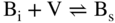
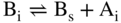
5.2.1.5 Interstitial–Substitutional Exchange Mechanisms
5.2.2 Diffusion at Chemical Equilibrium
5.2.3 Diffusion in a Net Chemical Flux
5.2.4 Condition of Limited Source
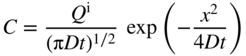
5.2.5 Conditions of Infinite Source
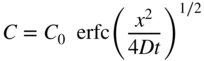
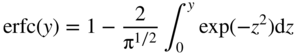
5.3 Diffusion Coefficients
5.3.1 Tracer Diffusion Coefficients
 is obtained from such an experiment.
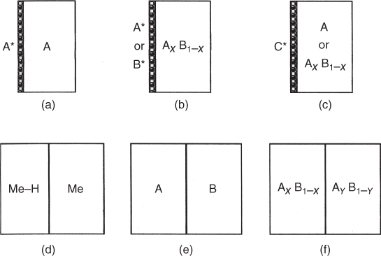
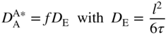
 and
and  . Both tracer diffusion coefficients will in general be different.
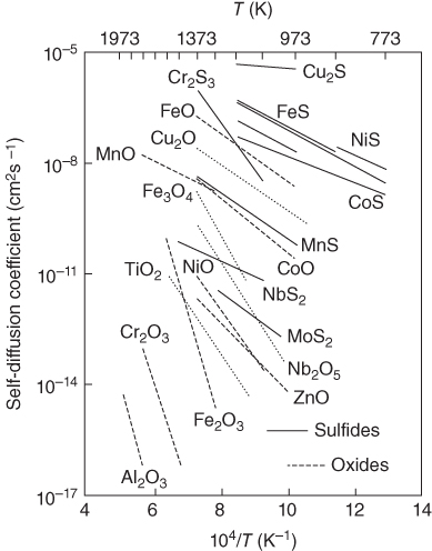
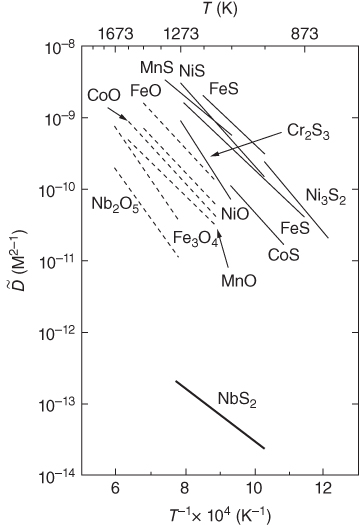
5.3.2 Chemical Diffusion (or Interdiffusion) Coefficient
 depend on T and p only. In this case, the gradient of the chemical potential is directly proportional to the logarithmic gradient of the concentration. In nonideal solutions, the gradient of the chemical potential gives rise to an “internal” driving force. As a consequence, the interdiffusion coefficient is concentration dependent, and Fick’s equation in the form of 5.10 must be used.

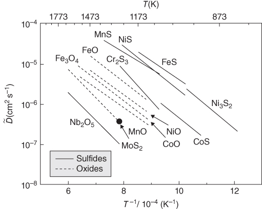
5.3.3 Intrinsic Diffusion Coefficients
 and the marker velocity vK (Kirkendall velocity). These relations were deduced for the first time by Darken (1948) and refined later on by Manning (1968). They will be discussed in Section 5.8. If the quantities
  and vK are known from experiment, the intrinsic diffusion coefficients can be deduced.
 and
and  are determined in a homogeneous alloy. In a metal–hydrogen system usually only H atoms are mobile. Then the intrinsic diffusion coefficient and the chemical diffusion coefficient of hydrogen are identical.
5.4 Matano–Boltzmann Analysis
 , at different compositions from the concentration profile measured by microprobe analysis. However, this method is restricted to systems where the partial molar volumes of the components are constant, i.e. the total volume does not change with reaction and mixing. Consider the case when two materials with initial compositions
  and
and  are coupled and annealed for reasonably short time, t, such that after annealing, still some part of the end‐members is not affected by the diffusion process as shown in Figure 5.11a. Boundary conditions can be written as

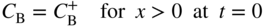
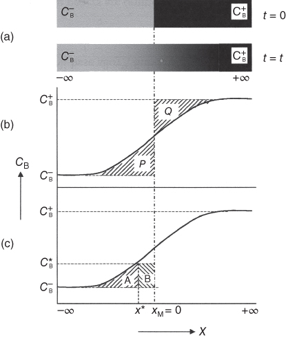
 and
and  before and after annealing for time t. (b) Matano plane xM = 0 can be found by equalizing the areas P and Q. (c) The value of the integral in Eq. 5.24 is equal to the shaded area (A + B) as shown in Eq. 5.26.
 to the concentration of interest to measure the interdiffusion coefficient,
 , at
, at  (
( ) leads to
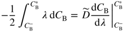
 and
and  . Using Eq. 5.20 one can write
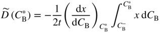
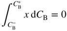
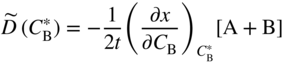
5.5 Kirkendall Effect
 , which is, in fact, a kind of average diffusivity of the elements, and it does not shed light on the diffusivities of the species, separately. In the early stage, it was common belief among researchers that diffusivities of the species are the same.
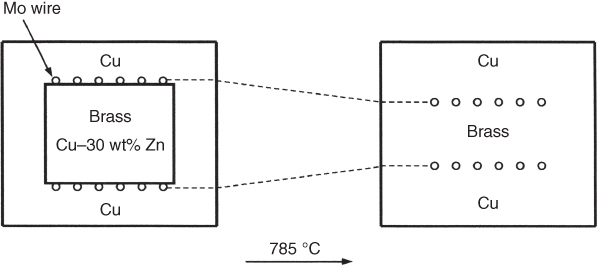
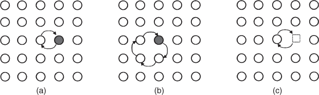
5.6 Darken Analysis
 and
and  as shown in Figure 5.14. Before annealing fiducial (inert) markers are introduced at the initial bonding interface and annealed at elevated temperature so that interdiffusion takes place. When interdiffusion starts, the markers will be trapped at a certain fixed composition and cannot escape at a later stage so that they move along with that fixed composition. If the intrinsic diffusivity of B (DB) is higher than the intrinsic diffusivity of A (DA) at that marker plane (called Kirkendall plane), then the Kirkendall marker plane will move to the right‐hand side from the initial contact interface, xM/0. The Matano plane, xM, is the initial contact interface when there is no change in total volume and is fixed with respect to the ends of the diffusion couple. This initial contact plane is denoted by x0 when volume changes upon reaction/mixing.
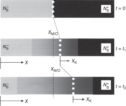
 and
and  demonstrating the Kirkendall effect. Inert markers (white spots) placed at initial contact interface before annealing are shifted with increasing annealing time (t2 > t1) to the right (from xM/0) as the diffusion of the species B is higher than the species A. The Kirkendall frame of reference, xK, moves with time, with respect to one end of the unreacted part of the specimen or with respect to xM/0 = 0.
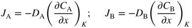
 and
and  (measured with respect to xM/0) and intrinsic fluxes JA and JB (measured with respect to the Kirkendall frame of reference at the position xK) can be written as

 and
and  are related by (using the relation VA dCA + VB dCB = 0)
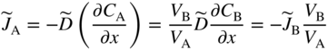
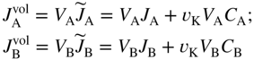
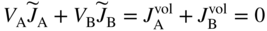
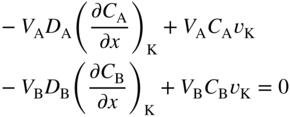
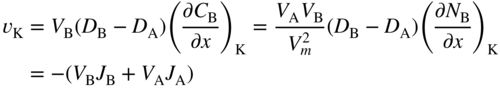
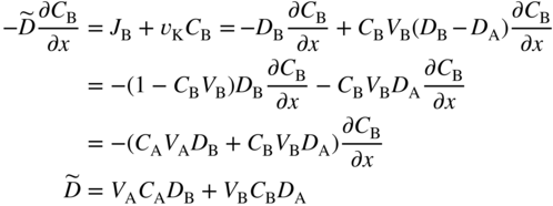
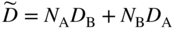
5.7 Factors Influencing Diffusion
5.7.1 Temperature Dependence
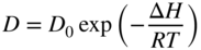
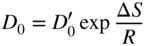
 contains geometric factors, the correlation factor, the lattice parameter squared, and an attempt frequency of the order of the Debye frequency.
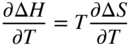
5.7.2 Pressure Dependence

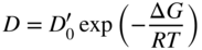
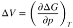
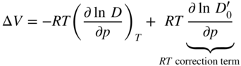
 can be estimated from the isothermal compressibility and the Grueneisen constant of the material. It is often negligibly small (a few percent of the molar volume Vm or of the atomic volume Ω = Vm/NA, respectively). Typical values for the activation volume for various metals lie between 0.5 and 0.9 Ω.
5.7.3 Other Factors Dependence
5.8 Impurity Diffusion in Metals
 and Di > Ds) the effective diffusivity reduces to the trivial case of interstitial diffusion:

 ), but the interstitial diffusivity is much faster than the substitutional one (Di ⋙ Ds). Then, the effective diffusivity (Eq. 5.44) approaches
5.9 Grain Boundary Diffusion in Metals
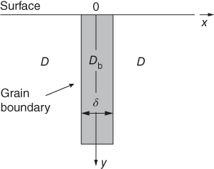
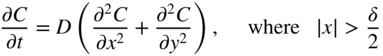
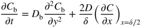

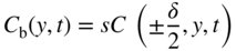

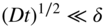
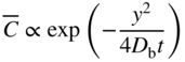
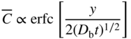
5.10 Diffusion in Solid Oxides
5.10.1 Brief Overview
 , and
, and  in CoO. In addition, the presence of a stoichiometric imbalance must, in some cases, be attributed not simply to one kind of defect, but rather to a combination of vacancies and interstitials. The predominant kind of defects and the change of those defects are a function of the oxide purity and of the temperature and oxygen pressure at which the oxide was prepared. Cation self‐diffusion studies have been particularly useful in aiding in the understanding of defect structures on the cation sublattice for oxides where cation defects are the minority atomic disorder, as in the case of UO2+x. For such oxides, little can be learned from measurements of electrical conductivity and weight change, which reflect effects due to the majority defects.
5.10.2 Diffusion in External Forces
 and
and  , are established on both sides of the oxide disk. As a consequence, a vacancy flux, jV, occurs from the high to the low oxygen potential side. Due to the flux coupling,
  , cations are driven in the opposite direction. When vacancies and cations arrive at the oxide surfaces, reduction and oxidation of the oxide occur at the low and high oxygen potential side, respectively:
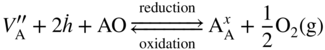
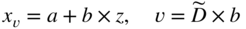
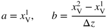
 . In a chemically homogeneous oxide without any gradients in chemical potentials, the diffusion fluxes vanish, and the drift flux can be written as
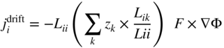
 or
or  , allows the determination of the effective charges of the corresponding cations, A or B. For self‐diffusion, i.e. tracers A*, we obtain
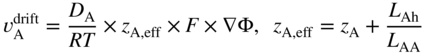
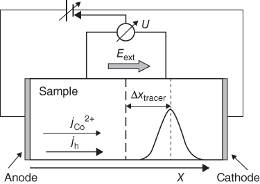
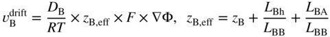
5.11 Morphology of Reaction Products
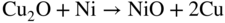
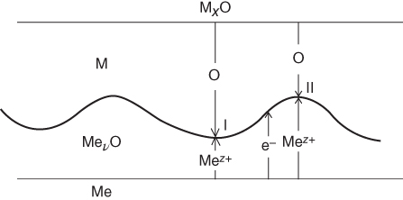
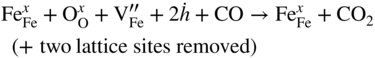
 ) toward the surface, which will be greater in the vicinity of a surface depression because of the shorter diffusion path. The higher concentration of vacancies in this region will be accompanied by a faster surface reaction as this process is proportional to the vacancy concentration (oxygen activity) (Engell 1958). According to this self‐enhanced reaction mechanism, a tunnel could readily develop from an initial depression on the surface. The enlargement of the surface area during the reduction of wüstite can proceed by this mechanism until the vacancy concentration in the wüstite approaches the value associated with the Fe/FeO equilibrium. While a similar model could be responsible for the tunnel structure produced in hematite, there is insufficient data about the surface reaction mechanism to confirm whether it would be enhanced by a flux of cation vacancies although this is probable. The reason for the change in mechanism responsible for the reduction of hematite as the temperature increases is not yet fully understood and provides an interesting problem for solid‐state chemistry.
5.12 Measurement of Diffusion Parameters
5.12.1 Junction Methods
5.12.1.1 Impurity Profiles
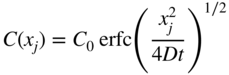
5.12.1.2 Chemical Etching
5.12.1.3 Electrochemical Plating
5.12.1.4 Scanning Light Spot
5.12.2 Electrical Methods
5.12.2.1 Four‐point Probe
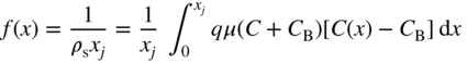

5.12.2.2 Hall Effect
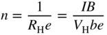

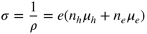
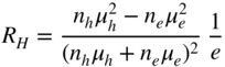
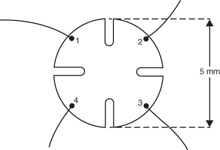
5.12.2.3 Diode Capacitance
5.12.3 Radiochemical Techniques
5.12.3.1 Radiotracer Analysis
5.12.3.2 Neutron Activation
5.12.4 Other Techniques
5.12.5 Calculation of D from a Profile

5.13 Questions and Problems
Temperature (°C)
Diffusion coefficient D (m3 s−1)
1380
3.11 × 10⁻¹⁴
1300
7.1 × 10⁻¹⁵
1250
4.1 × 10⁻¹⁵
1200
1.74 × 10⁻¹⁵
References
Further Reading
Diffusion in Solid‐State Systems
5.1
5.2
5.3
5.4
5.5
5.6
5.7
5.8
5.9
5.10
5.11
5.12
5.13
5.14
5.15
5.16
5.17
5.18
5.19
5.20
5.21
5.22
5.23
5.24
5.25
5.26
5.27
5.28
5.29
5.30
5.31
5.32
5.33
5.34
5.35
5.36
5.37
5.38
5.39
5.40
5.41
5.42
5.43
5.44
5.45
5.46
5.47
5.48
5.49
5.50
5.51
5.52
5.53
5.54
5.55
5.56
5.57
5.58
5.59
5.60
5.61
5.62
5.63
5.64
5.65
5.66
5.67
5.68
5.69
5.70