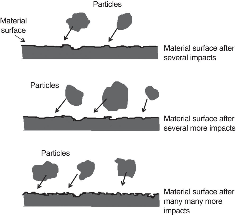
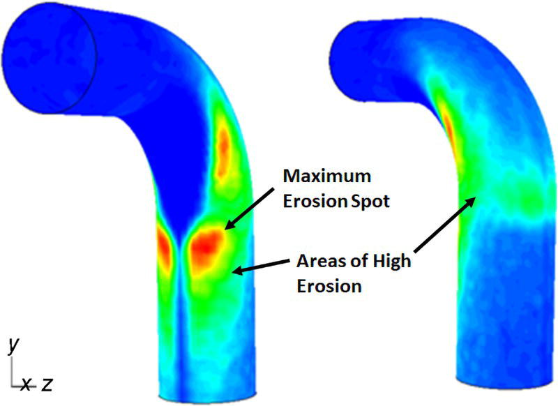
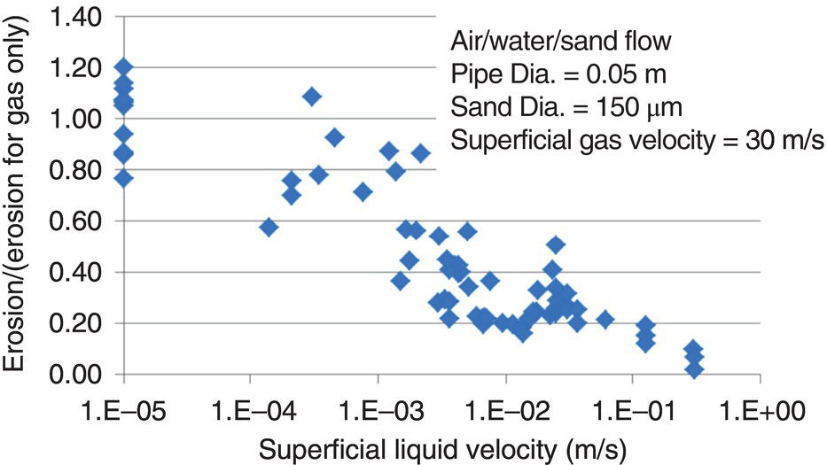
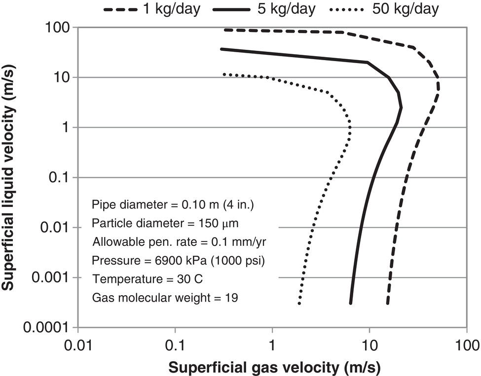
Siamack A. Shirazi1, Brenton S. McLaury1, John R. Shadley1, Kenneth P. Roberts1, Edmund F. Rybicki1, Hernan E. Rincon2, Shokrollah Hassani3, Faisal M. Al-Mutahar4 and Gusai H. Al-Aithan4 1Erosion/Corrosion Research Center, The University of Tulsa, Tulsa, OK, USA 2ConocoPhillips Company, Houston, TX, USA 3BP America Inc., Houston, TX, USA 4Saudi Aramco, Dhahran, Saudi Arabia Erosion–corrosion has many definitions. In all definitions of erosion–corrosion, there is a mechanical component—erosion, and an electrochemical component—corrosion, the two components working together to degrade metallic piping, tubing, and many other types of equipment. One of the most costly problems facing oil and gas production is related to material performance. According to a 2-year study conducted by the U.S. Federal Highway Administration (FHWA) on the cost of corrosion, the annual direct cost of corrosion in the oil and gas exploration and production industry is as high as $1.4 billion [1]. Also, the Department of Transportation Pipeline and Hazardous Materials Safety Administration (PHMSA) in significant incident files from 2012 reported corrosion to be the cause of 17.9% of all pipeline-reported incidents recorded from 1992 to 2011 [2]. Erosion–corrosion is not as common as other corrosion-related issues faced by the oil and gas industry, but it has been reported to be among the five main causes of failure with a 9% incidence of erosion–corrosion-related failures, following pitting (12%), preferential weld corrosion (18%), H2S-related (18%), and CO2 corrosion (28%). Thus, the understanding of erosion–corrosion in the oil and gas industry is indeed, quite relevant [3]. In most cases, the rate of metal loss is greater for the combined processes than for either erosion or corrosion working alone. Also, there are often significant interactions between erosion and corrosion. One useful way of defining the participation of the main components and their interactions in the total erosion–corrosion process is shown in Equation (61.1). In Equation (61.1), “erosion rate” refers to the rate of mechanical erosion of the metal, which would occur under the given conditions in the absence of an electrochemical corrosion component, and “corrosion rate” refers to the corrosion rate of the metal that would occur under the given conditions in the absence of a mechanical erosion component. For the two interaction terms in Equation (61.1), “effect of erosion on the corrosion rate” refers to the increment, positive or negative, that the corrosion rate undergoes when the full effect of the mechanical erosion component is considered, and “effect of corrosion on the erosion rate” is the increment, positive or negative, that the erosion rate undergoes when the full effect of the electrochemical component is considered. The term “synergy” is often used to describe cases for which the sum of the interaction terms ≠ 0.0, that is, when the erosion–corrosion rate given in Equation (61.1) is different from simply the sum of the erosion rate and corrosion rate. In oil and gas pipelines, the erodent is usually sand or another solid particle that is produced along with the production fluids. The most prevalent corrosion agent in oil and gas production and transportation is carbon dioxide gas dissolved in produced water. The presence of H2S gas, even in small quantities, is a major factor in the degradation of piping in production, gathering, and transportation systems, but is not so much associated with erosion–corrosion as is CO2. In many cases, the effect of corrosion on the erosion rate term in Equation (61.1) is small compared with the rates of the other erosion–corrosion components and can be neglected. In some erosion–corrosion systems, however, the effect of erosion on the corrosion rate can be very substantial, for example, when erosive forces strip away a corrosion product layer that would otherwise provide protection from corrosion. In these cases, the combined erosion and corrosion metal loss rate is larger than the sum of the loss rates from erosion and corrosion acting individually and often very much larger. Because the synergistic effect can be quite large, indeed, much larger than either the erosion or corrosion component, research on erosion–corrosion has favored systems involving a significant interaction term, and, usually this interaction term is the effect of erosion on the corrosion rate. In oil and gas pipelines, the erodent can be various produced particles or liquid drops entrained in a gas carrier fluid. However, the most common, and most destructive erodent is sand, so the mechanical partner in oilfield erosion–corrosion is most often sand erosion. In these cases, what is ultimately important is the so-called erosivity. Erosivity refers to the severity of the erosion conditions. Erosivity factors do not include properties of materials, but they include properties of the sand and carrier fluids, sand rate, flow conditions, and geometry. For example, increasing the sand rate would generally increase the erosivity. Because of the importance of solid particle erosion to understanding erosion–corrosion, the next section of this chapter focuses on the factors influencing solid particle erosion and on models developed to predict the erosion rate. Following the section on solid particle erosion, three erosion–corrosion processes are discussed, each involving an effect of erosion on corrosion that can result in an erosion–corrosion rate significantly greater than the sum of the erosion and corrosion rates taken separately. The first of these three erosion–corrosion systems, for which the effect of erosion on corrosion rate can be strong, involves erosion of a protective scale. In CO2-saturated systems, bare metal corrosion rates of carbon steel can be more than 800 mpy (20 mm/yr). However, under certain environmental conditions, an iron carbonate (FeCO3) scale can form on metal surfaces, which can reduce corrosion rates to a few mpy (0.1–0.2 mm/yr) [4]. Environmental conditions for which the protective iron carbonate scale is likely to form include pH > 5.0, temperature >150 °F (66 °C), plus a significant concentration of Fe2+ ions. When sand is entrained in the flow, impingement of the sand particles onto the iron carbonate scale can prevent the scale from forming or removing it completely or partially. As a result of this erosion of the scale, corrosion rates rise significantly or possibly return to bare metal values. A second example of a potentially very substantial effect of erosion on the corrosion rate involves corrosion-resistant alloys (CRAs). CRAs represent a class of iron-based materials that exhibit resistance to corrosion in many environments. Typically, a CRA will have a significant chromium alloying component and possibly many other alloying components as well. Most materials in this class work well in oil and gas production and transportation applications. When exposed to a corrosive environment, an oxide layer forms on the surface of the CRA, forming a barrier to the reactant species. In most particle-free oilfield fluids, the oxide layer is able to keep corrosion rates of the CRA at very low values. However, if sand or another solid particle is entrained, impingement of the particle onto the CRA can damage or partially remove the oxide layer, and increased corrosion rates may result. Erosion rate also can affect corrosion rate strongly in systems that are protected by a chemical inhibitor. The inhibitor in a liquid carrier fluid is injected into the system at the upstream end of the segment of piping that is to be protected. Typically, the inhibitor molecule attaches itself to the metal piping surface through adsorption. At a high enough inhibitor concentration, a barrier is created that sharply reduces the cathodic reactant penetration to the metal surface, keeping corrosion rates low. However, even at moderately high-flow velocities, entrained sand particles impinging on the metal surfaces can mechanically dislodge the inhibitor molecules from the surface, thereby exposing the bare metal, which leads to high corrosion rates. While much has been done to better understand erosion–corrosion and identify conditions where it will occur, it is important to note that attention to erosion–corrosion is relatively new when compared with the attention directed at understanding and controlling erosion and corrosion individually. Research on erosion and corrosion has helped build the foundation for the work on erosion–corrosion. The following sections introduce the reader to current testing and modeling approaches to better understand and mitigate metal loss in pipelines due to solid particle erosion and erosion–corrosion. During the production of oil and gas, solid particles are often present in the production fluids. The particles can be of sand or carbonate, which is released from the reservoir, or a material such as magnetite resulting from scale. The particles are a detrimental by-product of production and serve no favorable purpose. One potentially catastrophic result of the presence of particles is solid particle erosion, which can be defined as the mechanical removal of wall material by the impact of solid particles. Several removal mechanisms have been proposed, with three of the most common being cutting, fatigue, and brittle fracture. The authors have examined scanning electron microscopy (SEM) images from specimens eroded by sand for several materials used in the oil and gas industry such as carbon steels, stainless steels, titanium, and other materials such as aluminum, and the eroded surfaces look similar and provide insights into the typical erosion mechanism process. An SEM image of 316 stainless steel eroded by silica flour with a nominal diameter of approximately 25 μm, which has a wide range of particle sizes ranging mostly from 5–100 μm, is shown in Figure 61.1. Particles impinge the surface, creating craters pushing the material to the edges of the craters, creating lips of the material that are removed through subsequent impacts. Note that impingement of irregularly shaped 5–100 μm particles onto a steel surface can result in surface scratches and craters that are approximately 2–3 μm in length or diameter. Figure 61.2 shows a schematic of this process. However, removal of grains through fracture along grain boundaries has also been observed. Solid particle erosion is complex and not well understood. This is primarily due to the large number of factors that affect erosion and the difficulty in isolating the effect of a single factor. Considering particles flowing in a single-phase fluid, particle properties such as size, shape, density, and hardness; fluid properties such as density and viscosity; and characteristics of pipe wall material such as density and hardness all affect the severity of erosion. The problem becomes substantially more complex when particles flow in a multiphase carrier fluid due to the wide range of possible flow structures. When considering the effects of only particles and materials on wear process, Meng and Ludema [5] performed a literature study of wear equations and found 182 acceptable for analysis, 28 of which were specific to solid particle erosion. There were 33 different parameters in the 28 equations, with an average of five parameters in an equation. This demonstrates the level of incongruence among researchers. Figure 61.1 SEM image of Type 316 stainless steel (UNS No. S31600) eroded by silica flour. Figure 61.2 Schematic of the erosion mechanism commonly observed for ductile materials used in the oil and gas industry. Even though solid particle erosion is not fully understood, it is still necessary to estimate erosion rates or at least predict production velocities that would not cause excessive erosion. Historically, American Petroleum Institute-recommended practice 14E (API RP 14E) [6] has been used as a guideline to prevent significant erosion damage. This guideline provides an equation to calculate an “erosional” or a threshold velocity, presumably a flow velocity that is safe to operate. The recommended practice states that “The following procedure for establishing an ‘erosional velocity’ can be used where no specific information as to the erosive/corrosive properties of the fluid is available. The velocity above which erosion may occur can be determined by the following empirical equation: where: Industry experience to date indicates that for solids-free fluids values of c = 100 for continuous service and c = 125 for intermittent service are conservative.” The recommended practice adds “If solids production is anticipated, fluid velocities should be significantly reduced. Different values of ‘c’ may be used where specific application studies have shown them to be appropriate.” Unfortunately, this equation only considers one factor, the density of the medium, and does not consider many other factors that can contribute to erosion/corrosion in multiphase flow pipelines. It is obvious that Equation (61.2) is very simple and easy to use, but factors such as environmental conditions, fluid properties, flow geometry, type of metal, temperature, pH, sand production rate and size distribution, and flow composition are not accounted for. The only physical variable accounted for in Equation (61.2) is the fluid density. The equation suggests that the limiting velocity could be higher when the fluid density is lower. This does not agree with experimental observations for sand erosion or even for erosion caused by liquid droplets because sand and liquid droplets entrained in gases with lower densities will cause higher erosion rates than liquids with higher densities and viscosities. Therefore, the form of Equation (61.2) does not seem to be appropriate for many oilfield situations, including those involving sand production. Moreover, the basis for the development of the API RP 14E is not very clear. Salama [7] provides a review of many ideas and suggestions for the basis of the equation. Jordan [8] and McLaury and Shirazi [9] have compared the threshold velocities that were predicted by the API RP 14E to field data for c = 100 and concluded that the API equation is not conservative enough at high gas velocities and very low liquid rates. Recognizing the complexities involved in determining a suitable threshold velocity for controlling erosion and erosion/corrosion, many investigators are developing data and models for predicting erosion–corrosion. The API RP 14E equation with slightly different values of c is also proposed in ISO 13703 [10]. The origin of the expression is unclear, but it is unlikely that the original intent was to provide a criterion for solid particle erosion. However, this became the calculation of choice for oil and gas producers for many years probably due to ease of use and lack of other models, but it is apparent that many factors are not considered in the equation. In an attempt to overcome the shortcomings of API RP 14E, many companies developed tables of c values for use under various operating conditions. As a replacement for API RP 14E, other researchers developed other approaches to predict erosion or determine an erosional velocity specifically for solid particle erosion. Salama and Venkatesh [11] proposed an equation to predict the erosion rate as a function of sand rate, fluid velocity, material hardness, and pipe diameter. They further showed that the expression could be rearranged to provide an equation for erosional velocity for steel pipes with an allowable penetration rate of 10 mils/yr, as shown in Equation (61.3), where V is the erosional velocity in ft/s, d is the pipe diameter in inches, and W is the sand rate in barrels/month. The authors do note that this assumes the particles impact the pipe wall at velocities similar to the flow velocity, which may only be true for gases at low densities. Bourgoyne [12] also developed expressions for erosion rate prediction based on his experimental work. Equation (61.4) is his equation for penetration rate for dry gas or moist flow, where h is the erosion rate in m/s, Fe is a specific erosion factor (kg/kg) based on experimental results, ρa is particle density, ρs is the density of the wall material, qa is the volume flow of particles in m3/s, A is the cross-sectional area of the pipe in m2, Vsg is the superficial gas velocity in m/s, and Fg is the fractional volume of gas. A similar equation is also provided for liquid continuous flows replacing Vsg and Fg with Vsl, superficial liquid velocity, and Fl, fractional volume of liquid. Svedeman and Arnold [13] rearranged Bourgoyne’s equation to provide an erosional velocity assuming an acceptable erosion rate of 0.13 mm/yr (5 mils/yr), as shown in Equation (61.5), where Ve is the erosional velocity in ft/s, Ks is a fitting erosion constant, d is pipe diameter in inches, and Qs is the volumetric flow of solids in ft3/day. Ks accounts for several factors such as geometry type and material and phases present such as gas–sand, liquid–sand, or gas–liquid–sand. Salama [7] extended his work in erosion to develop an expression for erosion rate for particles in gas-liquid flows as a function of sand rate, mixture velocity, particle diameter, pipe diameter, mixture density, and an empirical value that accounts for geometry type and material. Assuming a sand size of 250 μm and an allowable erosion rate of 0.1 mm/yr (4 mils/yr), he rearranged the expression to solve for the erosional velocity in m/s, as shown in Equation (61.6), where S is a geometry-dependent constant, D is the pipe diameter in mm, ρm is the fluid mixture density in kg/m3, and W is the volumetric sand rate in kg/day. The models discussed to this point either assumed that particles impact at velocities close to the flow velocity or required empirical coefficients based on data, so applicability is extremely limited. In order to develop a more general approach, the particle impact velocity must be modeled. Currently, the most sophisticated approach to calculate erosion is the use of computational fluid dynamics (CFD). The larger, commercially available CFD programs have frameworks in place to predict erosion. The most common use of CFD for erosion prediction is an Eulerian–Lagrangian approach. The carrier fluid flow field is determined using an Eulerian method, and then individual particle paths are determined using a Lagrangian approach. Particle impact information, such as location, speed, and angle, is extracted during particle tracking and applied in an erosion equation. However, an Eulerian–Eulerian approach to predict erosion is also used where particles are treated as another phase instead of discrete entities. The CFD approach allows for calculation of erosion in complex three-dimensional geometries and provides a surface contour of erosion. Figure 61.3 displays a predicted erosion contour plot for a bend carrying liquid and sand particles. The areas pointed by arrows in the downstream section of the bend indicate the regions of high and maximum erosion. The maximum erosion for this specific condition is along the surface of the inner radius due to strong secondary flows that redirect particles to this location. The location of maximum erosion on an elbow for many cases is also expected to be on the outer radius of the elbow, but unusual cases such as that shown in Figure 61.3 could also occur. Figure 61.3 CFD prediction showing contour plot of erosion intensity in a bend carrying liquid and sand particles (left image is a view of the inner radius of the elbow; right image is a view of the outer radius of the elbow). CFD users must perform computational grid refinement studies to ensure that the flow field and particle motion are independent of the grid. For the Eulerian–Lagrangian approach, particle number studies must also be performed to ensure that a sufficient number of particles are examined to obtain statistically representative results. Another important factor for CFD simulations is an appropriate erosion equation. Erosion equations are typically determined experimentally and ideally are performed with the particles and wall material of interest. Data are commonly collected using a direct impingement (blasting) device at a variety of impact angles, as described in ASTM G-76 [14]. In order to control impact speed and angle, testing is normally performed in air. The particle rate in the tests must be low enough to avoid concentration effects such as particle–particle interaction or particles shielding the material being eroded. It is also mandatory that the particle velocity (if possible, impact velocity) be measured since the particle impact velocity can be significantly different than the average fluid velocity leaving the nozzle of the testing device. Zhang et al. [15] provide details on two forms of erosion equations commonly used in CFD simulations. The first form was developed by the Erosion/Corrosion Research Center (E/CRC) and is shown in Equations (61.7) and (61.8). ER is the erosion ratio in terms of mass loss of materials per mass of sand, Fs is the sand sharpness factor, Vp is the particle impact velocity, and F(θ) is the angle function. n = 2.41 is suggested by E/CRC, but others have suggested values between 1.5 and 3. C and A are empirical coefficients. BH is the Brinell hardness of the wall material. It is important to note that a general function of erosion with material hardness is not observed experimentally except within carbon steels for which this function was originally developed. So, for other materials, C(BH)−059 can be combined into one empirical coefficient. The second form was developed by Oka and is shown in Equations (61.9)–(61.11). E(θ) is the volume loss of the material divided by the mass of sand, E90 is the erosion at the normal impact angle; Hv is the Vickers hardness of the wall material; Vp and Dp are the particle impact speed and diameter, respectively; V ′ and D′ are the reference impact speed and reference particle diameter, respectively; n1, n2, and k2 are empirical functions of wall hardness; and K, k1, and k2 are empirical constants. It is apparent that there are several empirical constants contained in the equations to account for specific conditions used in the testing, but there are a couple of important similarities. Knowledge of the particle impact speed and angle is imperative. While CFD is an incredibly useful erosion prediction tool, there are disadvantages. Access to CFD programs must be available, and users must have a level of expertise. Additionally, significant progress has been made in the simulation of gas–liquid flows, but simulation of particles in gas–liquid flows still needs substantial development. So other simpler models or guidelines have been developed. One guideline is provided in DNV RP O51 [16]. This guideline provides erosion prediction in various geometries and states that the models presented are based on experiments and modeling efforts but warns that the data were generated at low pressures for relatively small pipe diameters. It appears that CFD was one of the tools used to generate the proposed models and for gas–liquid flows, mixture properties were used in the simulations. Due to difficulties of simulated gas–liquid flows, this is a common approach but often does not capture the effect of flow regime on erosion. Consider the erosion data shown in Figure 61.4 that are normalized to the gas-only condition, where erosion is shown as a function of superficial liquid velocity with constant superficial gas velocity. Superficial velocity is defined as the volumetric flow of that phase divided by the cross-sectional area of the pipe. The maximum erosion occurs for the gas-only condition and then decreases with the addition of liquid until the flow becomes annular, and then there is a slight increase and then decrease with further increase in the liquid rate. The increase and then decrease in liquid rate can be explained by examining the liquid film and the entrainment of liquid. As the liquid rate increases in this region, both the liquid film and the entrainment of liquid (and particles) increase. Initially, the increased entrainment is the dominant factor, so erosion increases since more particles are entrained in the gas core where velocities are higher. When the liquid rate increases further, the increased film thickness becomes the dominant factor, and the particle impact velocities reduce due to the increased film thickness. This behavior cannot be simulated assuming mixture properties. For low liquid rates, the predicted erosion values actually increase slightly from the gas-only conditions when applying mixture properties. Figure 61.4 Effect of liquid rate on erosion for a gas dominant flow. Another tool for erosion prediction is a program developed by the E/CRC at the University of Tulsa called Sand Production Pipe Saver (SPPS). This model has its origins in the early 1990s but has remained under continued development. The goal of the model is to predict a representative particle impact velocity for a set of conditions and then use this information in an erosion ratio equation to predict erosion. A simple one-dimensional particle tracking routine is used to predict the velocity of the particle as it passes through a one-dimensional fluid velocity field as the particle approaches the wall. When the particle is a radius away from the wall, the particle tracking routine is stopped and the particle velocity at that position is the impact velocity [17]. The length for which the particle tracking is performed is a function of the geometry type and size. Treating a three-dimensional flow in a one-dimensional manner has its limitations, especially for small particles and liquids, so a two-dimensional approach was also developed [18]. For gas–liquid flows, a similar approach to a single-phase carrier fluid is applied for flow patterns that are considered homogeneous, including churn and dispersed bubble. For annular [19] and slug flows [20], specific models are applied that account for the multiphase flow characteristics such as liquid film thickness and entrainment fraction for annular flow. Figure 61.5 shows the normalized predicted results using DNV RP O51 and SPPS for the data shown in Figure 61.4. Figure 61.5 DNV RP O51 and SPPS prediction trends of erosion for gas flow with low liquid loading. Figure 61.6 Comparison of allowable flow rates in an elbow using API RP 14E, SPPS, and DNV RP O501. SPPS and DNV RP O501 can also be used to predict flow rates that result in an allowable penetration rate. In this manner, results from SPPS can be compared with those of API RP 14E. Figure 61.6 displays such a comparison. In this figure, operating to the left of the curves is considered safe and operating to the right of the curves results in excessive erosion. Figure 61.6 illustrates a danger in applying API RP 14E. At low liquid rates, the allowable gas rate predicted by API RP 14E is too large. As the liquid rate reduces, the flow approaches gas only, which is a very erosive condition. It is important to mention that the API RP 14E results are independent of pipe diameter, sand size and rate, and allowable penetration rate. However, SPPS can be used to predict variations in threshold flow rates with these parameters. Figure 61.7 demonstrates the effect of sand rate using SPPS. The other conditions are the same as those used in Figure 61.6. Under some oil and gas production conditions involving a CO2 environment, an FeCO3 (iron carbonate) scale can form on carbon steel piping surfaces and provide considerable corrosion protection to the pipeline. But, if sand is entrained in the production fluids, sand particles impinging the walls of the piping and pipe fittings can cause erosion of the protective FeCO3 scale at particle impingement points and permit corrosion at bare metal rates. This type of erosion–corrosion is a particularly menacing form of metal loss because it can be more severe than either erosion or corrosion acting alone. Whether erosion–corrosion will be a problem in a particular oil and gas production situation depends on environmental (relating to corrosion) and mechanical (relating to erosion) factors. Figure 61.7 Effect of sand rate on threshold flow rates in an elbow using SPPS. For an iron carbonate scale to form, Equation (61.12) has to be satisfied at the surface of the metal where [Fe2+] and With the introduction of sand into the flow stream, erosion of the scale ensues. The scale may be thinned by the erosion, in which case some corrosion protection may be lost. At the same time, the FeCO3 scale is precipitating with the effect of growing the scale. Eventually, steady-state conditions are reached at which the scale deposition rate is equal to the erosion rate. Of course, for extremely high erosivities, the scale may be removed completely, in which case the corrosion rates return to bare metal values. Among the factors that determine the erosion rate of the scale are flow velocity, flow geometry, sand properties and sand rate, and erosion resistance of the scale. Factors that determine the deposition rate of the scale are the temperature and the supersaturation factor, SS, at the metal surface. The higher the value of SS, the higher the precipitation rate. The SS is given in Equation (61.13). Flow velocity is a parameter affecting both scale formation and scale reduction through dissolution and erosion. In many oilfield situations, flow velocity can be controlled to some extent by operational procedures. Shadley et al. [4] used a solid particle erosion model developed by Shirazi et al. [21] and results of erosion–corrosion testing in a laboratory flow loop to develop a semiempirical prediction model for erosion–corrosion in a carbon steel elbow in a CO2 environment with sand. The model provided an estimate of the “threshold velocity,” that is, the minimum flow velocity that would remove the scale for the given erosion and corrosion conditions. Figure 61.8 shows an example of how the threshold velocity and corrosion rate would change with increasing sand size. Threshold velocity falls sharply with sand size initially and then begins to level off for larger sand sizes. For a flow velocity of 3.8 m/s, the corrosion rates in this scenario would be very low for sand sizes <100 μm because an iron carbonate scale is providing good corrosion protection. Above 100 μm, the protective iron carbonate scale would be eroded away, eventually leading to bare metal corrosion rates for larger sand sizes. Figure 61.8 Threshold velocity and corrosion penetration rate (without considering the erosion rate) as a function of sand particle size. Test conditions were as follows: 205 kPa CO2, 74 °C, 5.5 pH, 10 ppm Fe2+, 5.0 kg/day sand production in a 76.2 mm diameter elbow, and 3.8 m/s flow velocity. One unexpected, but important outcome of the laboratory work behind the threshold velocity model was the finding that for flow velocities just above the threshold velocity, where the protective scale was intact in most places, but completely removed at sand impingement points, pitting was observed; and, in most cases, the pitting was quite severe. Figure 61.9 shows a photograph of two such specimens. These specimens formed the inner surface of the outside radius of elbows through which the sand-laden fluid flowed. The arrow in the photograph indicates the direction of flow. Often, at the test end, the iron carbonate scale would be observed on the upstream end of the elbow, but at the downstream end, the scale would be partially or completely removed by impinging sand. This finding defined three regions for corrosion behavior under scale-forming conditions: (1) low corrosion rates for flow velocities below the threshold velocity; (2) bare metal corrosion rates for flow velocities well above the threshold velocity; and (3) potential for severe pitting for flow velocities just above the threshold velocity. Figure 61.9 Examples of severe pitting in elbow specimens for cases slightly above the threshold velocity where the iron carbonate scale was removed at sand particle impingement points. For this geometry and other conditions tested, pitting most often occurred when pH was in the range 5.0 to 6.0. Test conditions were as follows: 80 °C, 450 kPappCO2, 0.5 wt% sand, 155 μm sand, 20 ppm Fe2+, 16 mm diameter elbow, 2% NaCl solution, 5.0 m/s flow rate at pH 5.5, and 2.0 m/s flow rate at pH 5.0. CO2 (sweet) corrosion is one of the major causes of tubing and piping failure in the oil and gas industry. In 2002, the total cost of failures due to corrosion was estimated to be approximately $7 billion annually in the United States [1]. Knowledge of damage risks is the first step in a program for controlling the costs of corrosion. Anticipating where corrosion is likely to happen, estimating its severity, and implementing suitable corrosion controls have become increasingly important in all phases of oil and gas extraction and transportation. Acquiring knowledge of the damage risks is the first step in an erosion–corrosion control program, and a model to predict where erosion–corrosion damage may occur and how severe the damage may be is an important tool toward achieving that objective. A model for an erosion–corrosion system in which iron carbonate scales provide significant corrosion protection must compare the rate at which iron carbonate scales are being deposited on the metal surface to the rate at which iron carbonate scales are being eroded from the metal surface. The rate at which iron carbonate scales are being eroded away depends on the erosivity of the system and the erosion resistance of the scale. The factors affecting the erosivity include sand properties, sand rate, carrier fluid properties, and flow rate. There are many factors that contribute to the formation and physical properties of the iron carbonate scale. These are discussed in the following sections. Increasing CO2 partial pressure increases the concentration of carbonate ions both in the bulk and at the metal surface due to increased corrosion rate, which in turn increases supersaturation. When supersaturation exceeds 0.0, the FeCO3 precipitation rate is proportional to supersaturation. The pH of the solution influences the formation of an iron carbonate scale in two ways: First, FeCO3 scales do not readily form when the pH is much lower than about 5.0 [22], and second, the scales formed at high pH are likely more protective and more erosion-resistant than scales formed at lower pH. When the temperature is lower than about 140 °F (60 °C), iron carbonate scales may not be observed due to the high solubility of iron carbonate [22]. For conditions for which supersaturation exceeds 0.0, the precipitation rate of the iron carbonate increases with increasing temperature. The higher the temperature, the more dense and protective is the scale. Shear stresses impressed on the metal surface by high flow velocity may mechanically disturb the formation of the iron carbonate scale. Furthermore, high flow velocity may reduce the supersaturation level at the metal surface through increased mass transfer of iron and carbonate ions away from the metal surface. Supersaturation increases by two ways, either increasing the concentrations of ferrous ions and carbonate ions at the metal surface or by decreasing the solubility product, Ksp. The solubility product is given by Equation (61.14) [23]. The solubility product increases with increasing absolute temperature, T, and solution ionic strength, I where ci are the concentrations of the various species in the aqueous solution in (mol/l) and zi are ion charges. The relations between the solubility product and temperatures for different ionic strengths are shown in Figure 61.10. Based on the aforementioned discussion, the scale is formed and deposited on the steel surface at different rates. Several models were developed for predicting scale precipitation and deposition rate [24–27]. The most influential factors controlling FeCO3 deposition rate (and supersaturation) are temperature and solubility product. When environmental conditions are right for forming the iron carbonate scale (FeCO3), the scale will deposit onto the metal surface. The scale microstructure and mechanical properties vary dependent upon the conditions under which the scale was formed [28, 29]. For example, the scale formed at 190 °F, 10 ft/s, pH 6.4, 2 wt% NaCl, 1900 parts per million (ppm) NaHCO3 eroded 5 times faster than bare mild steel tested under the same conditions of temperature, velocity, and erosivity. However, the scale formed at 150 °F, 10 ft/s, pH 6.24, 2 wt% NaCl, 1900 ppm NaHCO3 eroded 15 times faster than bare mild steel. The erosion rate was determined by the difference in weight and volume before and after the erosion. Test results are shown in Figure 61.11. Figure 61.10 The relation between the solubility of iron carbonate at different temperatures and ionic strength 0, 0.002, and 0.004 mol/l. Figure 61.11 Scale erosion rates and bare G10180 mild steel erosion rate. (Adapted from Ref. [30].) In the erosion–corrosion process, two different mechanisms contribute to the metal loss of the pipe or tubing. The first one is through the anodic reaction in the corrosion process. The second mechanism is the removal of the metal surface as a result of erosion by sand particle impingement. The sand particles in the carrier fluid impact the pipe surface, causing chipping and gouging. Under scale-forming conditions, the iron carbonate scale may cover the metal surface. In this case, it is the FeCO3 scale that is eroded, and the corrosion that is taking place is merely replacing the scale at places where the scale has been thinned due to the erosion. Figure 61.12 shows the results of many tests, in which FeCO3 scales were formed, and then sand was entrained in the flow stream. The figure shows that when sand erosion rates were 0 or low, the corrosion rate (corrosion part of erosion–corrosion) was very low. However, when erosion rates were increased, corrosion rates increased sharply. In some cases, the iron carbonate scale was completely removed, allowing corrosion to take place at bare metal rates. Al-Mutahar et al. [31] developed a model to predict steady-state erosion–corrosion rates. A flowchart of the erosion–corrosion model procedure is shown in Figure 61.13. A sand erosion prediction model [31] is used to estimate the erosion rate of the iron carbonate scale. A CO2 corrosion rate prediction model [31] was modified to estimate the corrosion rate under scale-forming conditions. A third model was developed that combined the erosion and corrosion models and computed the corrosion rate under steady conditions. The sequence of the computational process can be summarized in the following steps for thermodynamic conditions that are favorable for iron carbonate scale formation: Figure 61.12 Corrosion part of the erosion–corrosion process showing increase with increase of erosivity at two different testing conditions. (Adapted from Ref. [30].) Figure 61.13 Flow chart of the erosion–corrosion model computational procedure. (Adapted from Ref. [31].) As a further illustration of how the erosion–corrosion model works, a sample calculation is presented in this section for a multiphase flow in a 90° elbow. For the case described in Table 61.1, the CO2 corrosion model predicts that the scale was likely to form under these thermodynamic conditions. The erosion rate of the scale was then predicted using the erosion rate prediction model. Figure 61.14 shows the erosion rate of the iron carbonate scale computed for a range of superficial gas velocities. Next, the steady-state scale thickness is calculated. The steady-state scale thickness is the thickness at which the formation rate of the iron carbonate scale equals the erosion rate of the scale. Figure 61.15 shows the formation rate of the scale computed over a range of scale thicknesses. For a formation rate of the scale equal to 0.27 mm/yr (equal to the predicted erosion rate), the steady-state scale thickness is predicted to be 6 μm. Finally, the corrosion rate is calculated for the steady-state scale thickness of 6 μm, which is much thicker than that of stainless steel oxide, which is <10 nm. Figure 61.16 shows the corrosion rate computed over a range of scale thicknesses. For a 6 μm scale thickness, the predicted material corrosion rate is 1 mm/yr (≈40 mpy). Table 61.1 Flow Conditions for Multiphase Case Figure 61.14 Prediction of the erosion rate of the scale for the multiphase case described in Table 61.1. (Adapted from Ref. [31].) Figure 61.15 Prediction of the formation rate of the scale and steady-state scale thickness for the multiphase case described in Table 61.1. (Adapted from Ref. [31].) Further details of model development are described by Al-Mutahar et al. [31] and Al-Aithan [30]. Figure 61.16 Prediction of the steady-state corrosion rate for the multiphase case described in Table 61.1. (Adapted from Ref. [31].) In general terms, CRAs are defined by the Specification API 5CRA/ISO 13680:2010 as “alloy intended to be resistant to general and localized corrosion and/or environmental cracking in environments that are corrosive to carbon and low-alloy steels.” This definition is very broad, including the alloy families of martensitic, duplex, austenitic, and precipitation-hardened stainless steels and Ni alloys as well as titanium alloys. Most of these alloy groups have excellent resistance to CO2 corrosion, but they may suffer from other damage mechanisms such as pitting corrosion by oxidants, environmental-assisted cracking, and other depassivation-related damage mechanisms, including erosion–corrosion. For some applications, it may be more economical in the long term to use CRA instead of the more commonly used carbon steel with inhibitors. Recently, the industry has witnessed the increasing use of CRAs in oil and gas production tubing. In a sweet environment, the most widely used CRA for downhole tubular application is martensitic stainless steel 13Cr-L80 and its modified types. The main reason for its broad usage is its excellent corrosion resistance to flow-assisted CO2 corrosion. In fact, the effects of high gas velocity on carbon steels in carbon dioxide environments are reduced to a low level or virtually eliminated by alloying with 12% or more chromium [32]. Also, the relatively low cost of 13Cr stainless steel compared with that of alloys such as Duplex stainless steel or more costly Ni Austenitic alloys makes the martensitic stainless steel a very attractive option. Some studies have been conducted on 13Cr to explore the interactions between sand particle erosion and CO2 corrosion in a flowing two-phase (water/CO2 gas) system. Erosion corrosion resistance of the 13Cr alloy family may be significantly better than that of carbon steel under certain conditions (see Figure 61.17 [33]). At low erosivity conditions such as low velocities, single-flow liquids with sand concentrations as high as 5–7%, 13Cr has shown erosion–corrosion rates within industry acceptable limits for long-term service (as low as 5 mpy). At similar erosivity conditions, carbon steel may experience erosion–corrosion rates much higher than bare metal CO2 corrosion rates and as high as 1 inch of wall thickness lost per year. In such conditions, erosion–corrosion rates are dominated by the corrosion component of the damage mechanism. Even at low erosivity conditions, removal of pseudo-protective iron carbonate layers on carbon steel by the mechanical action of solid particle impingements can increase metal loss rates to rates higher than bare metal corrosion rates (see Figure 61.18 [34]). Figure 61.17 Comparison between the erosion–corrosion penetration rate for carbon steel and 13Cr in single-phase liquid conditions. ([33]/with permission of NACE International.) Figure 61.18 Corrosion rate (LPR on horizontal to down plugged tee) for carbon steel under scale-forming conditions (Vsg = 10 ft/s (3.1 m/s), Vsl = 3.5 ft/s (1.1 m/s), T = 195 °F (91 °C), pH 6.2, and initial [Fe2+] = 10 ppm). (Adapted from Ref. [34].) At similar conditions, the 13Cr is still able to either maintain its passivating film or to repassivate fast enough (re-healing of the Cr–Fe oxide layer) to hold the total metal loss rate to within acceptable limits. This remains true for multiphase flows involving CO2 and sand as long as the erosivity of the sand-bearing fluid is relatively low. Figure 61.19 [35] shows the similarity between the pure erosion rates and erosion–corrosion rates of 13Cr exposed to multiphase flow conditions at background (very low) sand concentrations. Note that the 95% confidence intervals of the total metal loss rate based on five measurements for both pure erosion (distilled water, sand, and inert N2) and erosion–corrosion (CO2-saturated brine and sand) overlap to a large extent. At these flow rates and sand concentration combinations (erosivities), both pure erosion and erosion–corrosion remain low and well within acceptable long-term penetration rate limits. Figure 61.19 Penetration rates for pure erosion and erosion–corrosion tests of 13Cr in the multiphase flow at 76 °F (24.4 °C). The error symbols for the average of the data represent the 95% confidence interval on the mean value. (Adapted from Ref. [35].) When erosivity conditions are severe enough, that is, either flow rates are too high or solid particle concentrations are high, the removal of passive films in some CRAs could overcome the ability of the passive film to reform enabling large erosion–corrosion rates. When the erosion–corrosion rates are larger than the pure erosion rates and the pure corrosion rates added as if they were taking place separately, the system is said to behave synergistically, that is, the whole is greater than the sum of the parts. Figure 61.20 illustrates this concept for 13Cr L80 exposed to high flow rates combined with high sand production rates at room temperatures. At lower pH and higher temperatures, the effect would likely be larger [35]. Other researchers have found similar behaviors in other martensitic stainless steel tested under different sets of conditions [36]. This mechanism has been of concern to the industry. Erosion–corrosion damage of this type and the likelihood of failure can be controlled by limiting flow rates (but, with great economic impact due to limiting of the production rate), or by better down hole sand control measures or through appropriate material selection if the potential problem can be recognized in the early stages of the project. Figure 61.20 Annular flow: VSG = 97 ft/s; VSL = 0.2 ft/s sand rate ~48 lb/day; N2 or CO2, T =76 °F; 13Cr. (Adapted from Ref. [35].) Other, higher alloyed CRAs, such as super martensitic stainless steel, have shown reduced synergistic effects of erosion–corrosion as compared with the 13 Cr-L80; and at similar conditions, higher-grade alloys such as cold-worked duplex stainless steels can completely curb the synergistic effect at severe erosivity conditions for pure erosion rates as high as 100 mpy. Of course, at erosion rates this high, it would likely be necessary to control flow rates and/or solid concentrations to reduce the pure erosion rates to acceptable limits as well [37] (see Figure 61.21). On a side note, it is worth taking notice from this figure of the proximity of the values of pure erosion rates for 13Cr-L80, Super 13Cr-95, and 22Cr-110 in spite of their differences in Rockwell C hardness values (22 HRC, 28 HRC, and 36 HRC, respectively). Hence, although the erosion–corrosion resistances of different CRA grades could be significantly different, their pure erosion resistance is very similar. Therefore, it is not recommended to anticipate better resistance to erosion due to higher hardness when working within this range of engineering alloys. In fact, the typically higher mechanical properties of the CRAs have justified the use of thinner piping for a given mechanical design requirement. A thinner wall permits less reaction time to avoid loss of containment should a severe erosion event occur due to temporary production of sand, thus increasing the risk of failure. These considerations should be taken into account, while designing high production facilities or service with risk of sand production. Figure 61.21 Erosion–corrosion (EC), pure erosion (pureE), and corrosion component of the erosion–corrosion (CEC) penetration rates at 150 °F. (Adapted from Ref. [37].) Significantly greater hardness may yield significant reductions in erosion rates as in the use of Co, Ni, and tungsten carbides alloys in the form of intermetallic laves phase alloys, hard facing alloys, or carbide-strengthened alloys, hence their success when used as inserts in choke valves in high flow or sandy services or drilling tools in severe wearing service [38]. The effect of hardness on erosion resistance alloys has also been proved, but once again, even large changes in hardness for low-alloy steels with diverse heat treatments have shown little effect on erosion resistance [39] (see Figure 61.22). A laboratory method previously introduced by McMahon and Martin [40] was also used by Rincon [35] to study the effect of pH and temperature on the repassivation behavior of CRAs in CO2-saturated brine. The laboratory method was conducted in a glass cell. Data were collected based on an electrochemical technique. The working electrode (CRA) is scratched, while the potential and current are recorded. After some simple mathematical calculation, Rincon et al. [37] showed that thickness loss and repassivation time can be estimated. The scratch made on a well-defined area of the working electrode may be interpreted as similar to the removal of the passive layer due to a single-particle impingement, and, it is believed that this approach can be used to study the effect of erosion on the corrosion response. With scratch tests, the mechanical process making the scratch and the repassivation process of a CRA can be viewed as nearly separate events. The sand erosion process bears some similarity to a simple scratch test, except that mechanical and electrochemical processes involved are taking place simultaneously and continuously. The goal of investigating the simple scratch test was to shed some light on the erosion–corrosion behavior of CRAs. The effects of pH and temperature on the repassivation of 13Cr, Super 13Cr, and 22Cr were examined in previous research periods. Figure 61.22 Erosion resistance (1/volume eroded in mm3) as a function of Vickers hardness for several pure metals and steels with diverse work hardening and heat treatments. (Adapted from Ref. [39]. Data from Finnie, I., Wolak, J. and Kabil, Y., 1967, Journal of Materials, 2, 682–700.) Figure 61.23 Decay of the anodic current for three different alloys. (Adapted from Ref. [37].) For a typical scratch test of an active passive alloy, the anodic current is very high immediately after making the scratch. How fast the current decays with time depends on the healing rate of the oxide film, which depends on the alloy grade as well as environmental conditions such as corrosive agent, pH, and temperature (see Figures 61.23–61.25). Figure 61.23 shows a comparison of current responses among the three CRAs at a temperature of 150 °F. Scratch tests made at 76 and 200 °F indicate that the ranking of the alloys is the same regardless of the temperature. For a given pH and temperature, the current response, and thus the corrosion rate, for Super 13Cr, is much lower than the one for 13Cr but not as low as for 22Cr. As expected, the Super 13Cr is performing better than 13Cr, but not as well as 22Cr. Figure 61.24 shows the current decays for 13Cr at 76 °F for different pH conditions. A couple of trends can be seen in this figure. The current decays at faster rates at higher pHs, as indicated by the greater (more negative) initial slopes shown for pH 5.25 and 6 as compared with lower pH (3.5 or 4). Also, the value of the current observed is lower for higher pH (5.25 or 6) than for lower pH (3.5 or 4) over the entire interval of 200 s shown in the figure. Since the corrosion rates are proportional to the current, these results suggest very high corrosion rates immediately after making the scratch and exposing the bare metal to the corrosive solution. Then, the corrosion rates decay with time, while the healing process takes place on the metallic surface. The passivated state is achieved sooner for higher pH. For higher temperatures, namely, 150 and 200 °F, similar trends are observed (results were presented by Rincon et al. [33, 35]). However, the initial currents obtained immediately after making the scratch for these temperatures are much higher than the current obtained for 76 °F. Figure 61.25 shows the comparison of the current decays at different temperatures; 76, 150, and 200 °F at pH 4. As expected, at higher temperatures, higher healing rates were found, as suggested by the steeper slopes shown by the current versus time curves at 200 °F. However, the higher temperature always causes a current that is initially higher and remains higher over the entire test period. As a result, at higher temperatures, it takes longer time for the current to return to its original level. It has been shown that the anodic current decay over an initial repassivation period can be characterized as approximately following the second-order behavior expressed by Equation (61.15): Figure 61.24 Effect of pH on the decay of the anodic current after scratching the surface of a 13Cr Alloy. ([41]/Rincon, Hernan E.) Figure 61.25 Effect of temperature on the decay of the anodic current after scratching the surface of a 13Cr Alloy. ([41]/Rincon, Hernan E.) where I is the measured current, t is time, and m is a constant that depends on material and environmental conditions. Integration of Equation (61.15) yields a convenient form for characterizing the healing process (repassivation process). The first integration yields where I0 is the initial current at t = 0. Equation (61.17) can be used to compare the repassivation responses of a particular alloy under different environmental conditions or to compare the repassivation responses of several alloys exposed to a particular environment. The comparison of material B (or environment B) to material A (or environment A) can be done according to the thickness loss (TL) accumulated by the time the corrosion rate reduces to (near) 0 as follows: where the subscripts A and B refer to materials (or environments) A and B, respectively, TLRB/A is the ratio of thickness losses between the two materials (or environments), C is a units conversion factor, and I* is the value of the current at a given time lapse, t* after the scratch has been made. This means that knowing m and I0, one can predict the time required for the corrosion current to return to the value of interest, I*. If I* is set to correspond to a corrosion rate of, for instance, 1 mpy, Equation (61.17) can be used to estimate the cumulative metal loss experienced by the alloy during the repassivation process between the time of the scratch and the time the corrosion rate returns to 1 mpy. Taking the limit of the thickness loss ratio as the final current I* approaches 0 yields the thickness loss ratio simply equal to mA/mB. IA and IB in Equation (61.17) refer to the initial (t = 0) corrosion currents for material (or environment) A and material (or environment) B, respectively. The second-order model was found to be a very good approximation to describe the repassivation process of stainless steels such as 13Cr and 22Cr under all pH and temperature combinations for a CO2-saturated solution for at least the first 200 s after the scratch. Figure 61.26 shows the cumulative thickness losses from current responses shown in Figure 61.25. As expected, and proved elsewhere ([33, 35]) with flow loop testing data, thickness losses are shown to be higher for higher temperatures. The same trends are obtained for pH 3.5, 5.25, and 6.0, but results are not shown in this chapter. Table 61.2 shows flow loop test values and predicted values of the corrosion component (Ce–c) of the erosion–corrosion penetration rates for three alloys tested at similar conditions (76 °F (24.4 °C), pH 4). The predicted values were obtained by means of Equation (61.17) where material A is 13Cr and material B is S13Cr or 22Cr. As can be seen, the loop test and predicted Ce–c values match very well for both S13Cr and 22Cr, suggesting that scratch data as used in Equation (61.17) may be useful to predict erosion–corrosion penetration rates, provided that data from at least one loop test are available for similar erosivity and environmental conditions. Similar analysis has been done for other temperatures and pHs using Equation (61.17) and scratch test slopes, m, indicating reasonable agreement between flow loop test values and predicted values. The testing predicting methodology already discussed has been used as an effective and efficient procedure for investigating the erosion–corrosion behavior of CRAs in oilfield environments. The main idea was to reduce the need for expensive and time-consuming loop tests by using a simplified scratch test. Figure 61.26 Comparison of the cumulative thickness loss of the 13Cr alloy after being scratched at pH = 4.0. ([41]/Rincon, Hernan E.) Table 61.2 Loop Test Values and Predicted Values of the Corrosion Component (Ce–c) of the Erosion–corrosion Penetration Rates for three Alloys Tested at Similar Conditions (76 °F (24.4 °C), pH 4) Source: [37]/with permission of NACE International. a Obtained by subtracting the erosion rate from the erosion–corrosion rate. A novel procedure to predict erosion–corrosion of CRAs using the second-order model and scratch test along with solid particle impinging data generated from CFD simulations was proposed by Rincon [41]. Figure 61.27 shows the comparison between experimental data and predicted values for erosion–corrosion rates of three CRAs. The figure shows how a model [41] based on Equations (61.15)–(61.17) was able to grasp the trends for the erosion–corrosion behavior of the three alloys with respect to CRA type and temperature. These results are encouraging, especially when considering the complexity of the phenomenon under study and the large number of variables taken into account in the model. The previous section showed the breakdown of the total erosion–corrosion weight lost as the summation of four different components. Changes in exposure conditions, such as flow velocity, sand rate, and alloy grade with different chemistry or microstructure, could affect each component differently, shifting the damage mechanism dominance and, therefore, the total waste loss rate. This phenomenon was observed by He et al. [42] when studying the erosion–corrosion behavior of four different stainless steels with a diverse range of chemistry, microstructure, and microhardness. Under the experimental conditions of this study, the corrosion component was a small contributor to the total erosion–corrosion weight loss. The mechanical removal action of the solid particle impingements produced most of the weight loss. Thus, the microstructure and respective microhardness proved to be significant factors in the total erosion–corrosion resistance, shifting the ranking of the alloys with changes in the acidity of the media and flow velocities. Aribo et al. [43] conducted studies to compare the erosion–corrosion performance of lean duplex stainless steels, (UNS S32101) and austenitic steel 304 stainless steel (UNS S30403). Lean duplex steels appear to have better resistance to erosion and erosion–corrosion damage than austenitic stainless steels when exposed to flows having velocities of 15 m/s and containing 500 mg/L of sand. The generality of this trend is still subject to verification by consideration of a broader experimental matrix. XRD spectra analysis for fresh surfaces and sand-flow exposed surfaces for these two alloys demonstrated that sand impingement was able to induce enough stress to transform some of the austenite volume fraction to an α-martensite, causing an increase in localized hardness on both austenitic and the lean duplex stainless steel alloys. The extension of the microstructure phase transformation seems to be related to the erosion and erosion resistance of these alloys and their relative ranking with regard to erosion–corrosion resistance. More research studies in this area are needed to improve the prediction of erosion–corrosion rates of CRAs. Figure 61.27 Comparison between experimental data and predicted trends of the erosion–corrosion, EC of the three CRAs at two different temperatures. (All data normalized to 13Cr at room temperature value.) ([41]/Rincon, Hernan E.) At high erosivity conditions, a synergistic effect between erosion and corrosion was confirmed in three CRAs (13Cr-L80, Super13Cr-95, and 22Cr-110) since the total metal loss rate was shown to be higher than the sum of the rates of corrosion (without sand) and erosion measured separately. It appears that under the high sand rate conditions tested, the erosivity is severe enough to damage the passive layer, thereby enabling the raised corrosion rate. Synergism seems to occur for the three alloys; however, the degree of synergism is quite different for the three alloys and may not be significant for 22Cr under field conditions where erosivities are typically much lower than those occurring in the small bore loop used in this testing. For the other two alloys, 13Cr and Super13Cr, especially at high temperatures, if the erosion rate of the passive film is great enough, then an accelerated erosion–corrosion process may take place with a significant contribution from a corrosion component. In most cases, there is likely a competition between the protective film removal due to mechanical erosion and the protective film healing. If erosivity conditions are severe enough, the base metal can also be removed by the mechanical erosion component. A mechanistic model of this competition would need to account for film characteristics, the concentration and distribution of sand, the flow pattern and flow velocities, flow geometry, and environmental factors. Predictions of the corrosion component of erosion–corrosion based on scratch test data compared well to test results from a multiphase gas/liquid flow loop for the three CRAs at high erosivity conditions. Second-order behavior appears to be an appropriate and useful model to represent the repassivation process of CRAs. A procedure to predict penetration rates for erosion–corrosion conditions was developed based on the second- order model behavior observed for the re-healing process of the passive film of CRAs under tested conditions. Good agreement between the actual and predicted penetration rates was found. Application of chemical inhibitors is one of the most common and successful practices for controlling corrosion and erosion–corrosion in the oil and gas industry. Considerable research in the oil and gas industry has been devoted to the development of inhibitor systems that can reduce corrosion rates in production equipment to acceptable levels. There are many different types of inhibitors that are used for the oil and gas industry applications. Imidazoline-based inhibitor is commonly used by oil and gas companies for sweet corrosion applications. Several commercial inhibitors have been developed by chemical companies to mitigate corrosion, especially for CO2 and H2S systems. Some of these inhibitors are claimed to be useful for erosion–corrosion mitigation as well. There are several parameters affecting the inhibitor performance, including pH of solution, flow velocity and flow regime, temperature, sand erosion, oil/water emulsion, metal cations, chlorides, type of metal, and electrolyte [44–54]. The effect of sand erosion on inhibitor performance is an important area of concern in oil and gas production because inhibitors that are effective in a CO2-saturated static brine are not necessarily effective under erosion–corrosion conditions [55]. Sand production also increases the inhibitor concentration needed for optimum inhibitor effectiveness [47]. In this section, the effect of sand erosion on inhibitor performance and also prediction of the inhibited erosion–corrosion rate as a function of environmental conditions will be discussed in detail. Reduction of chemical inhibition performance by sand erosion has been reported by several authors [53, 54, 56–59]. Interactions of sand particles with chemical inhibitors in oil and gas wells depend on different parameters, including inhibitor characteristics, sand type, sand size, and presence of oil in the system. In general, this interaction has been explained by mechanical removal of inhibitors from the surface and also by reducing the effective inhibitor concentration in the system. McMahon et al. [60] experimentally showed that large amounts of corrosion inhibitor can be lost from the bulk solution by adsorption of the inhibitor onto the surfaces of produced sand particles. This can reduce the concentration of the inhibitor that is available to protect steel surfaces. However, this effect only becomes significant for high concentrations of sand (>1000 ppm) and small particle sizes (<10 μm diameter), especially for oil-wetted particles [60]. On the other hand, Ramachandran et al. [61] showed that the effect of inhibitor loss due to sand adsorption is small for industrial corrosion inhibitors used under field conditions. Tandon et al. [56] showed that inhibitor protection provided by concentrations of 100 ppm and above was not affected much by the addition of small amounts of sand under non-scale-forming conditions. However, for some inhibitor concentrations, increasing sand concentration adversely affected the ability of the inhibitor to maintain optimum protection over extended periods of time [56]. Using an inhibitor can change the erosion–corrosion behavior. Shadley et al. [62, 63] showed that using an effective inhibitor can increase the threshold velocity for removal of an iron carbonate scale in a carbon steel elbow in the CO2-saturated brine solution. The velocity limit below which the scale can be maintained is defined as the “threshold velocity.” Working above the threshold velocity, pitting or uniform corrosion can occur. At velocities below the threshold velocity, a protective scale can form on pipe walls, and metal loss rates are typically low. The upward shift of threshold velocity provides a much larger scale formation region and, thus, greater flexibility in piping system design and operation. Tummala et al. [55] studied two inhibitor treatment scenarios involving the preexisting iron carbonate scale: in the first scenario, sand was added to the system 1 day after adding the inhibitor; and, in the second scenario, the inhibitor was added to the system 1 day after adding sand. In both scenarios, adding sand increased the corrosion rate and reduced the inhibitor performance, but final corrosion rates were the same—about 0.5 mm/yr. The chemical inhibitor added to the system before or after sand entrainment shows the same efficiency. However, inhibitor efficiency is reduced because of the sand interaction. The need to be able to predict inhibitor performance under sand production conditions is particularly acute when the wells are deep or offshore because of the difficulty in running coupon tests to evaluate the inhibitor efficiency at critical points throughout a system, which might involve a number of wells flowing into a single header. Further, it would be highly desirable to be able to make decisions on the design of the well, given advanced knowledge of the inhibition options and their predicted effectiveness. Crossland et al. [64] suggested a correlation for the prediction of the likelihood of erosion–corrosion inhibition success in the oil and gas industry as a function of environmental factors such as temperature, shear stress, and total dissolved solids Equation (61.18). This correlation is a statistical correlation based on experimental and field data over a wide range of production conditions, but it does not include the effects of sand production. They defined four different regions for inhibitor performance, which can be used for the estimation of the amount of the inhibitor needed to get the corrosion rate lower than 0.1 mm/yr (Table 61.3) [64]. where ILSS is the inhibitor likelihood success score and TDS is total dissolved solids. Al Zawai et al. [65] used the response surface method design to model the erosion–corrosion rate as a function of sand load, flow velocity, and inhibitor concentration. They conducted the erosion–corrosion experiment using a jet impingement geometry for three different sand loads (SL = 150, 500, and 1500 ppm), flow velocities (V = 7, 10, and 20 m/s), and inhibitor concentrations (CI = 0, 100, and 150 ppm) in order to develop an empirical model for erosion–corrosion prediction. Equation (61.19) is an empirical correlation for prediction of erosion–corrosion rate in the inhibited system based on total weight loss (TWL). Table 61.3 Summary of Inhibition Risk Categories and Guidance Source: [62]/with permission of NACE International. Hassani et al. [53, 54] developed a methodology for prediction of the inhibited erosion–corrosion rate, which is a combination of the sand erosion model, CO2 corrosion model, and modified inhibitor adsorption isotherm. There are several factors involved in this model, including sand erosion parameters (sand size, sand shape, sand density, sand concentration, flow velocity, geometry, flow regime, fluid density, and viscosity) and CO2 corrosion parameters (temperature, pH, CO2 pressure, flow velocity, and regime). Erosion–corrosion consists of two parts: the erosion part of erosion–corrosion and the corrosion part of erosion–corrosion. The erosion part can be predicted by predicting pure erosion and erosion affected by corrosion. The corrosion part also has two components, including pure corrosion and corrosion affected by erosion. Corrosion can affect erosion by changing the surface roughness and also by forming corrosion products on the surface, which may have a different erosion resistance in comparison with the base metal. Erosion can also affect the corrosion behavior by removing the corrosion products from the surface, removing the corrosion inhibitor from the surface, and also changing the surface morphology. Erosion–corrosion, involving solid particles, is a complicated phenomenon, and many factors affect erosion–corrosion mechanisms and the synergistic effects that occur between the erosion and corrosion of mild steels. Addition of inhibitors adds another order of complexity to the phenomenon. However, in order to make engineering predictions of erosion–corrosion with inhibitors, some simplifying assumptions have to be made. Hassani et al. [53, 54] experimentally showed that for CO2 corrosion of carbon steel, erosion affected by corrosion can be neglected in comparison with total the erosion–corrosion rate (Hatched area in Figure 61.28). Harvey et al. [66] also neglected this term in the erosion–corrosion prediction modeling. Using this assumption, the erosion part of erosion–corrosion is equal to the pure erosion rate, which can be predicted using pure erosion prediction models. The corrosion part can be predicted by combining the pure CO2 corrosion prediction model with a modified inhibitor adsorption isotherm to predict the corrosion part of the erosion–corrosion. The pure CO2 corrosion rate can be predicted using the available mechanistic models. However, corrosion affected by erosion was predicted using a modified inhibitor adsorption isotherm. The Frumkin inhibitor adsorption isotherm was modified by including an erosivity term in the adsorption/desorption constant (Equation 61.20). Figure 61.28 Effect of inhibitor concentration on the erosion–corrosion rate and its components at T = 57 °C, pH = 4.8, pCO2= 2.4 bar, and the target material is X65 carbon steel. ([53]/with permission of NACE International.) where Ka/d is the adsorption/desorption constant, ER is the erosion rate, ΔT is temperature change, Cinh is inhibitor concentration, θ is surface coverage by the inhibitor, and f is an adjustable parameter accounting for the interaction between adsorbed inhibitor molecules. The adsorption/desorption constant is the best term for including the effect of erosivity since it is a function of entropy of the system. Entropy is an expression for randomness and disorder in the system, and sand erosion causes randomness and disorder in the inhibitor adsorption/desorption process. Therefore, the total erosion–corrosion rate can be predicted by predicting the pure erosion rate, pure CO2 corrosion rate, and effect of sand erosion on inhibitor performance (i.e., modified inhibitor adsorption isotherm). Figure 61.29 shows a comparison between experimental and predicted erosion–corrosion rates as a function of inhibitor concentration and temperature when the erosivity of the system (erosion rate of mild steel) is about 4 mm/yr. Figure 61.29 Comparison between experimental data and prediction of the total erosion–corrosion rate as a function of inhibitor concentration at T = 57 and 93 °C, pH = 4.8, pCO2 = 2.4 bar, and the target material is X65 carbon steel. ([53]/with permission of NACE International.) The oil and gas production industry has long recognized that corrosion and erosion can damage flow lines, elbows, chokes, valves, headers and other flow lines, and production equipment. More recently, the process of erosion–corrosion has received increased attention as a damaging process. The erosion–corrosion process involves both erosion and corrosion and is inherently more complex than erosion or corrosion. There are several conditions where erosion–corrosion can cause severe damage to metallic flow components. One condition occurs after a protective corrosion scale has been formed on a carbon steel, and sand erosion removes the scale in a localized area to bare metal. The localized area of the bare metal acts like a small anode, and the scale area acts like a large cathode, resulting in severe pitting, see Figure 61.9. Another erosion–corrosion condition occurs with CRAs, which have a thin protective oxidation layer. Sand erosion can remove this layer and again expose the bare metal to cause increased corrosion rates. A third condition is when inhibitors are used and the sand production is severe enough to damage the inhibitor protective coating. Tests show corrosion rates increase for this condition. Much has been done in the past two decades to determine procedures for dealing with erosion–corrosion. Threshold velocities have been determined identifying the flow velocities above which pitting is a risk. Models and experimental tests to predict erosion of metals for a variety of flow regimes, flow geometries, particle sizes, and fluid properties have been or are being developed. These tools, coupled with corrosion models and flow analysis, are being applied to erosion–corrosion problems. Studies on the erosion removal of corrosion scales have been successful, which is an important step toward developing possible procedures for predicting erosion–corrosion-induced pitting. While important steps have been taken and progress has been made, there are still challenges to meet in increasing the level of understanding of erosion–corrosion, before it reaches the levels of application that corrosion or erosion have attained. The authors wish to acknowledge the support of over 50 oil and gas and service companies that have supported the E/CRC since 1982, and many project monitors from these companies who have contributed to the research of the E/CRC. The authors especially acknowledge Mr. Edward Bowers, Senior Technician of the E/CRC for his ideas, design, construction, and maintenance of all 12 of the flow loops and other test equipment in the E/CRC and for guiding students in their research.
61
Erosion–Corrosion in Oil and Gas Pipelines*
61.1 Introduction
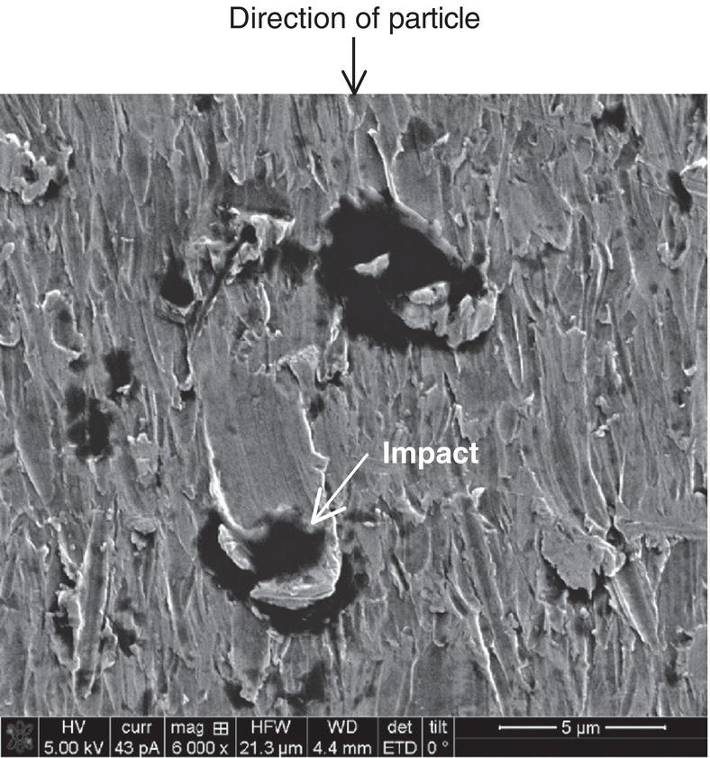
61.2 Solid Particle Erosion


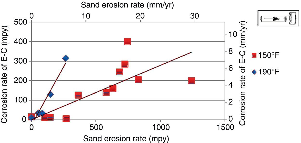
61.3 Erosion–Corrosion of Carbon Steel Piping in a CO2 Environment with Sand
 are the molar concentrations of iron and carbonate ions, respectively, at the metal surface, and Ksp is the solubility product of FeCO3. This condition usually requires the temperature to be above 150 °F (66 °C), the pH to be above 5.0, and a supersaturation of Fe2+ ions. Iron carbonate scales formed at temperatures near or above 200 °F (93 °C) are nonporous and tough. Scales formed at these temperatures may be only a few micrometers in thickness and still provide excellent protection against corrosion. Scales formed at lower temperatures tend to be more porous and to exhibit cracking and possibly separation from the metal substrate. But, they can be much thicker than the higher-temperature scales. Corrosion protection is typically lower for the lower-temperature scales, but in some cases still significant.
61.4 Erosion–Corrosion Modeling and Characterization of Iron Carbonate Erosivity
61.4.1 CO2 Partial Pressure
61.4.2 pH
61.4.3 Temperature
61.4.4 Flow Velocity
61.4.5 Supersaturation
61.4.6 Erosion of Scale
61.4.7 Erosion–Corrosion
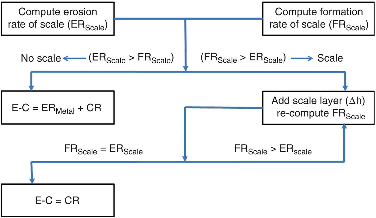
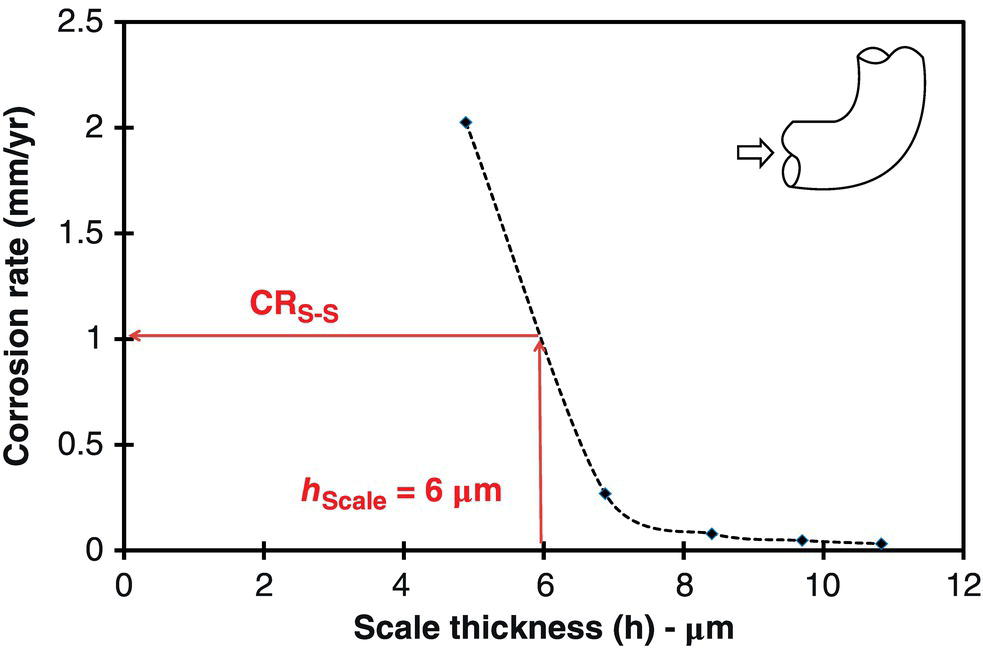
61.4.8 Erosion–Corrosion Model Development
Geometry
90° Elbow
Diameter
89 mm
Temperature
90 °C
p CO2
4.5 bars
V sl
3.0 m/s
V sg
10.0 m/s
pH
5.9
[Fe2+]
10 ppm
NaCl
3 wt%
Sand rate
36 kg/day
Sand size
150 μm
Sand shape
Semi rounded 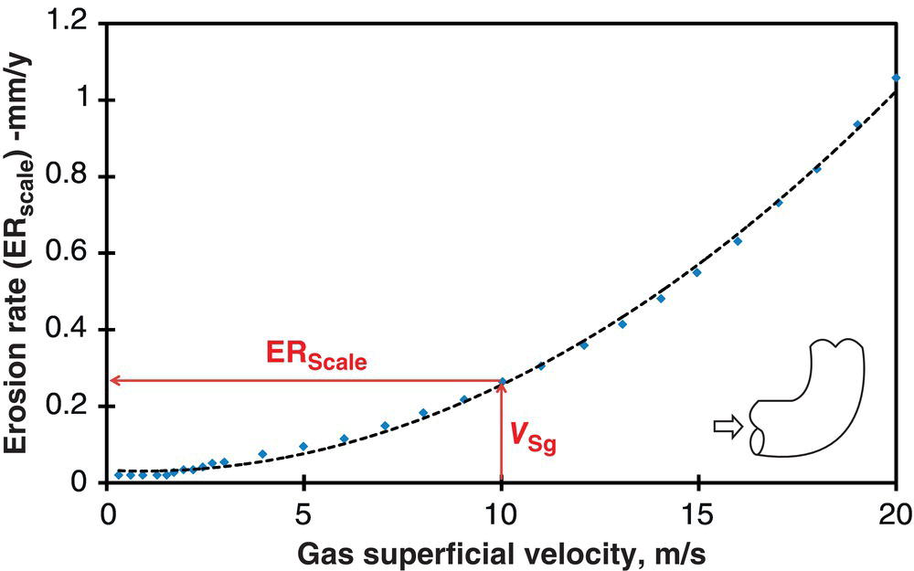

61.5 Erosion–Corrosion of Corrosion-Resistant Alloys
61.5.1 Erosion–Corrosion of Carbon Steels Versus CRAs
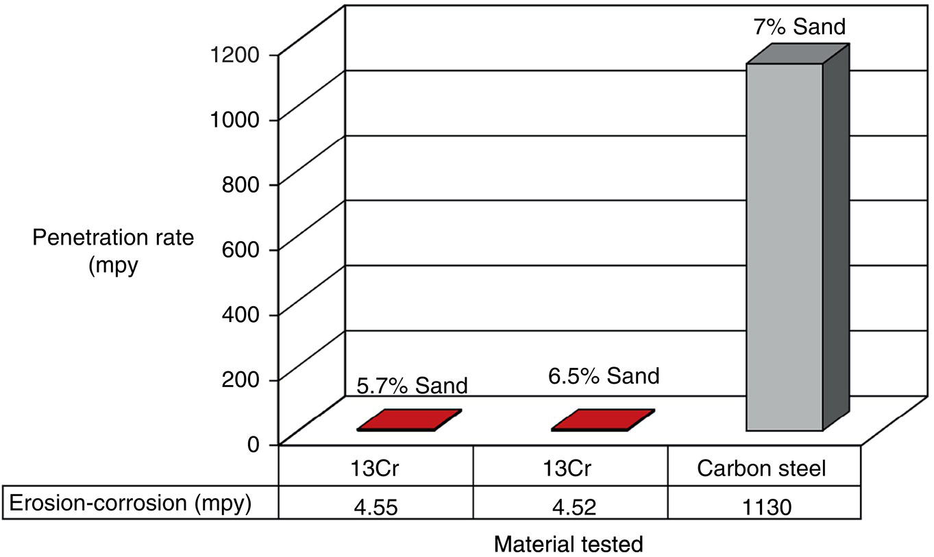
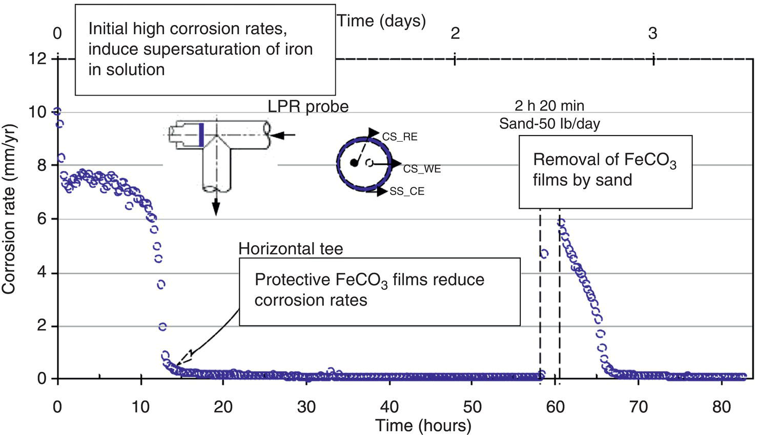
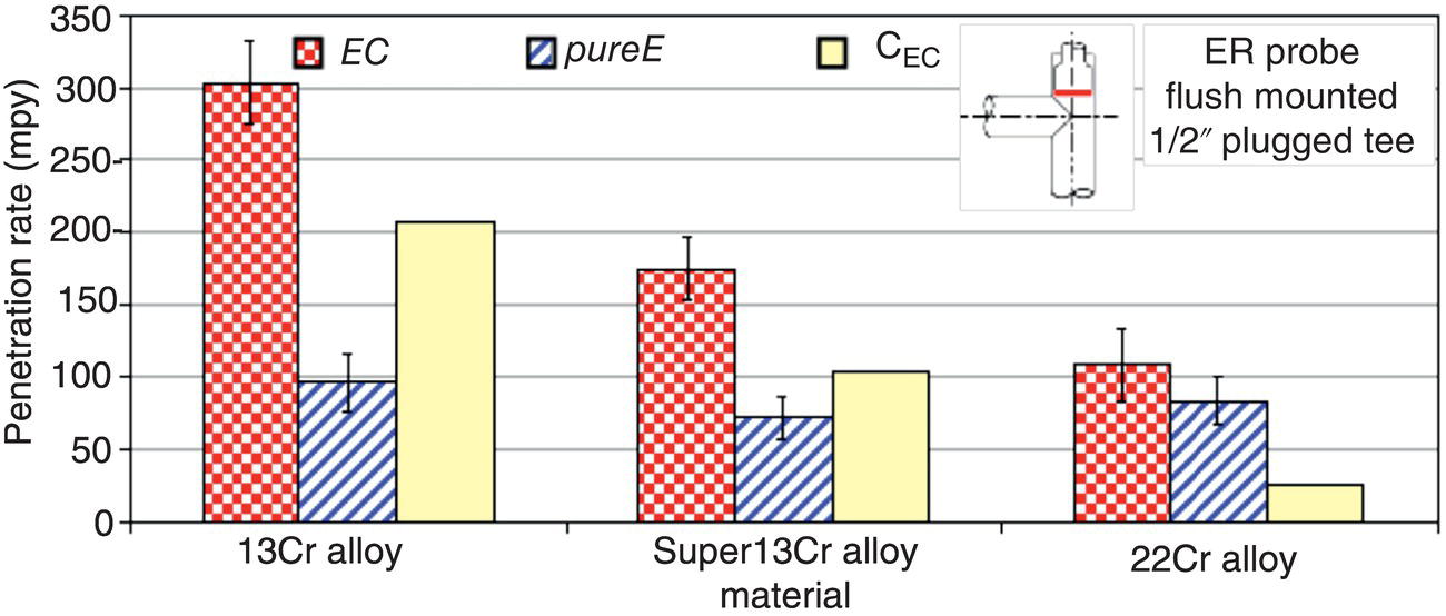
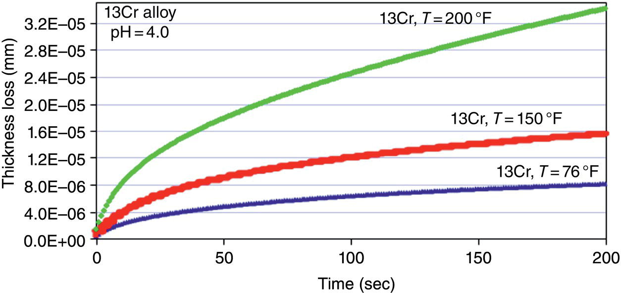
61.5.2 Erosion–Corrosion with CRAs Under High Erosivity Conditions
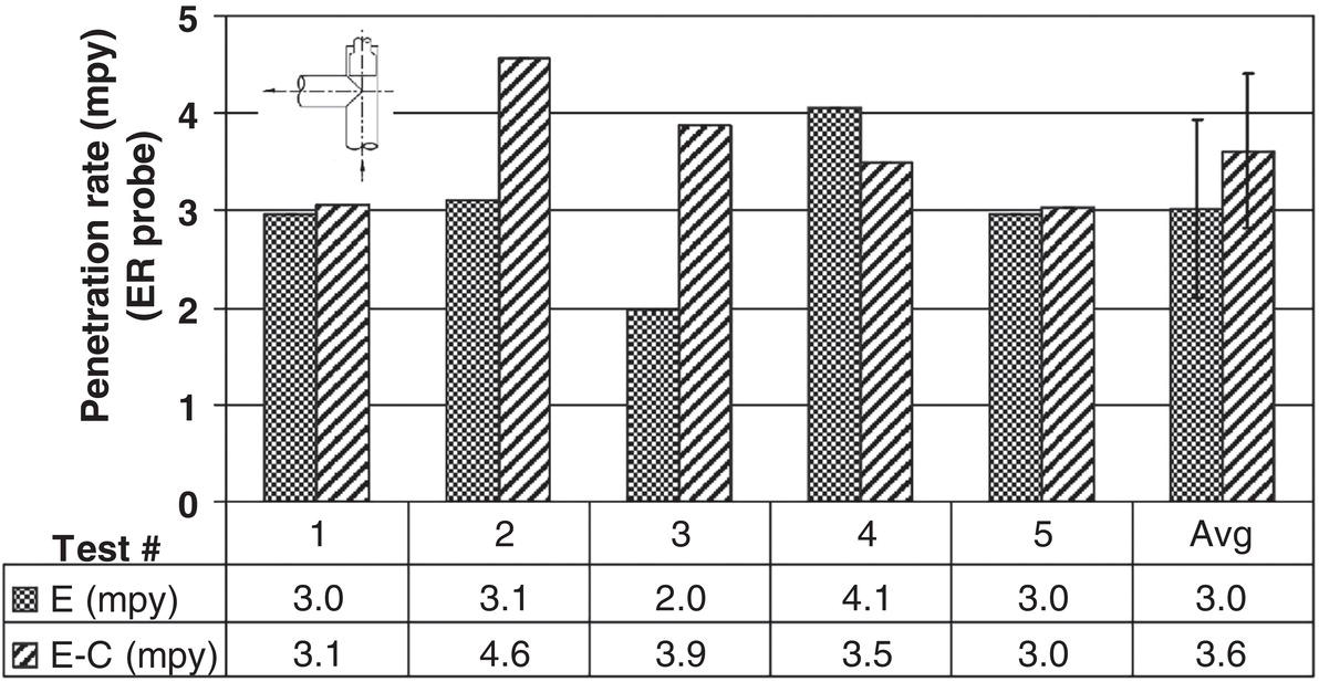
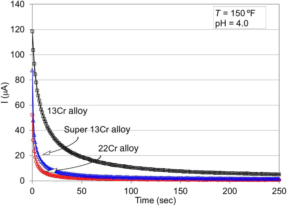
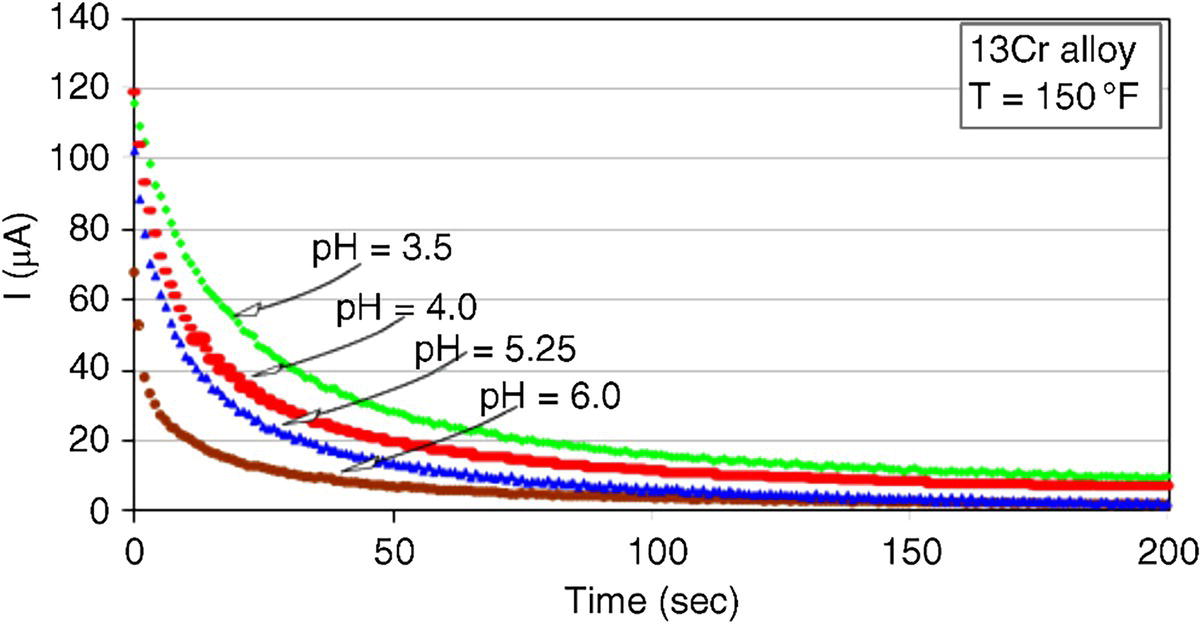
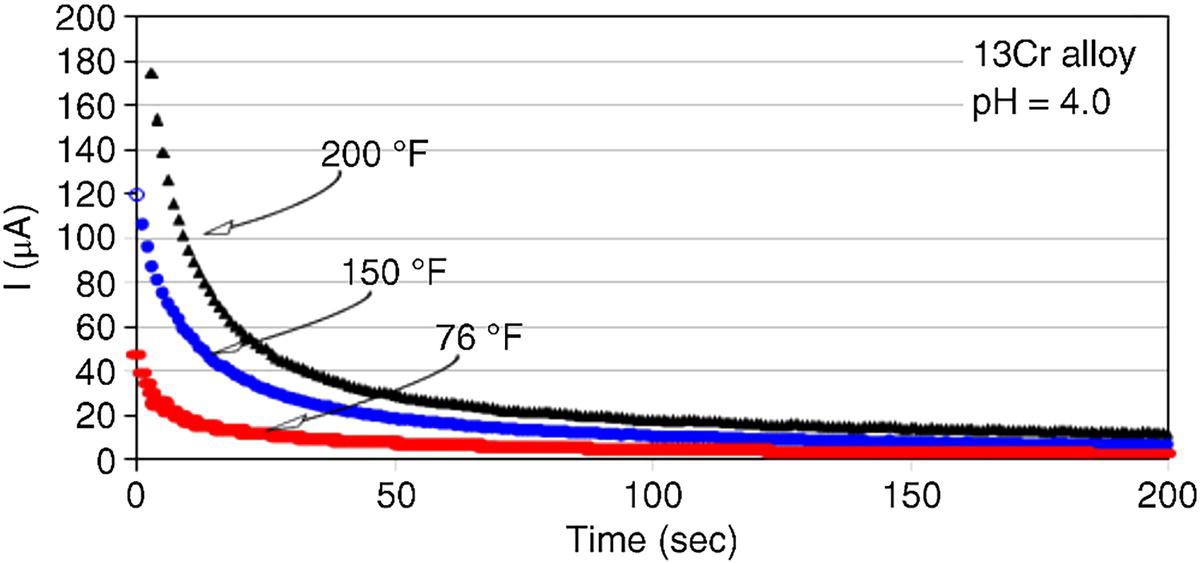
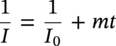
61.5.3 Repassivation of CRAs
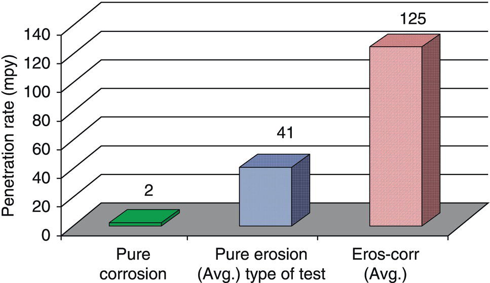
Alloy
Loot test Ce–c rateaCe–c = EC–E (mpy)
Scratch test data TLRB/A = (m13Cr/mCRA)
Predicted Ce-c rate Ce–c,CRA = TLRB/ACEC,13Cr (mpy)
13Cr
99
1
(Reference)
Super13Cr
47
0.40
40
22Cr
29
0.22
22
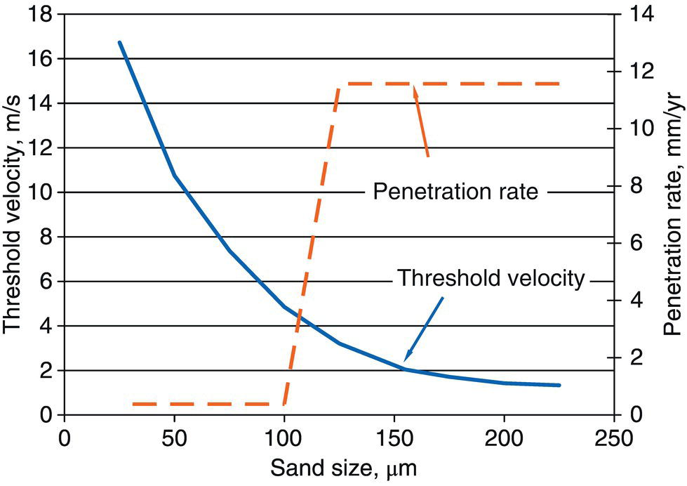
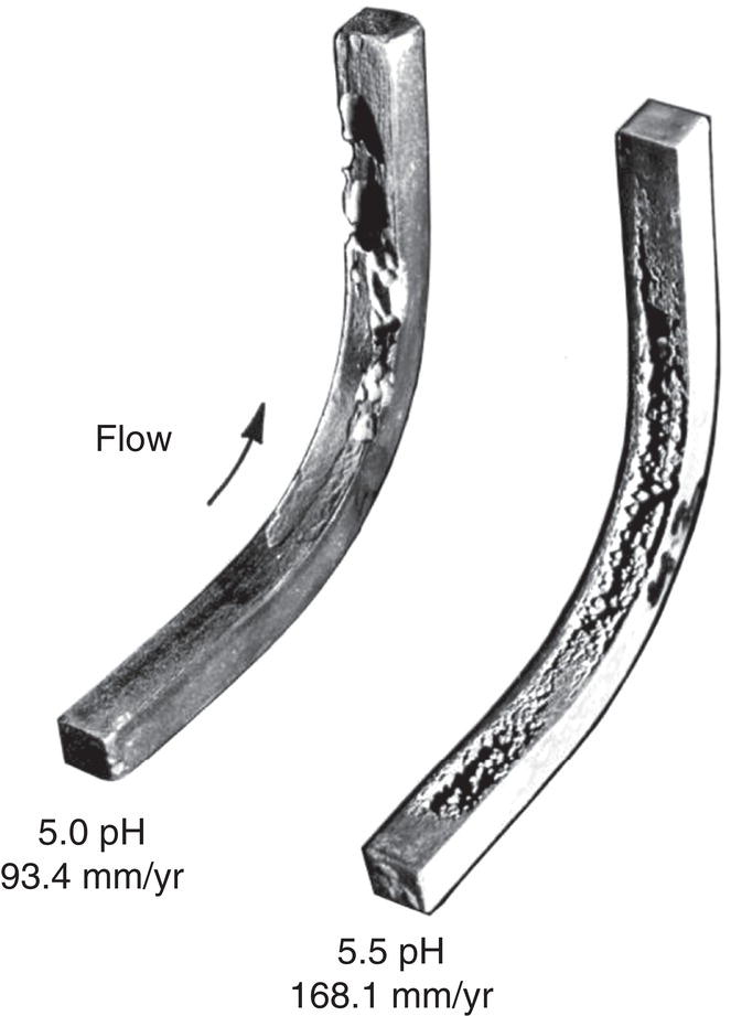
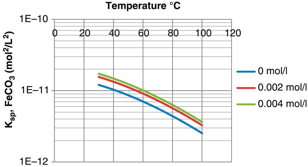
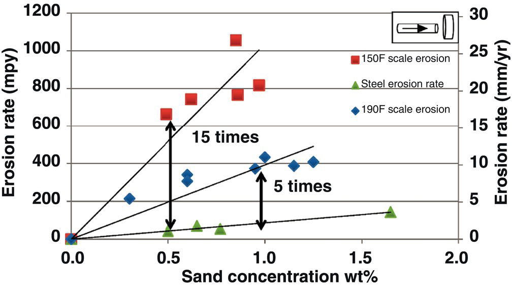
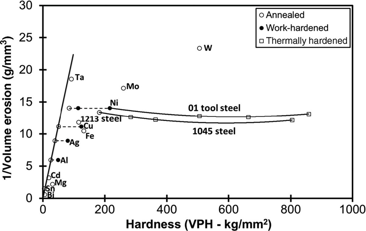
61.5.4 Effect of Microstructure and Crystallography on Erosion-Corrosion
61.5.5 Summary
61.6 Chemical Inhibition of Erosion–Corrosion
61.6.1 Effect of Sand Erosion on Chemical Inhibition
61.6.2 Modeling and Prediction of Inhibited Erosion–Corrosion
Category
ILSS
Description
1
ILLS < 2.5
Corrosion inhibition success is highly likely (inhibitor concentration up to 50 ppm)
2
2.5 < ILSS < 4
Corrosion inhibition success is expected (inhibitor concentration up to 100 ppm)
3
4 < ILSS < 5.5
Corrosion inhibition is challenging (inhibitor concentration up to 300 ppm)
4
5.5 < ILSS
Corrosion inhibition may not be viable (inhibitor concentration more than 400 ppm)
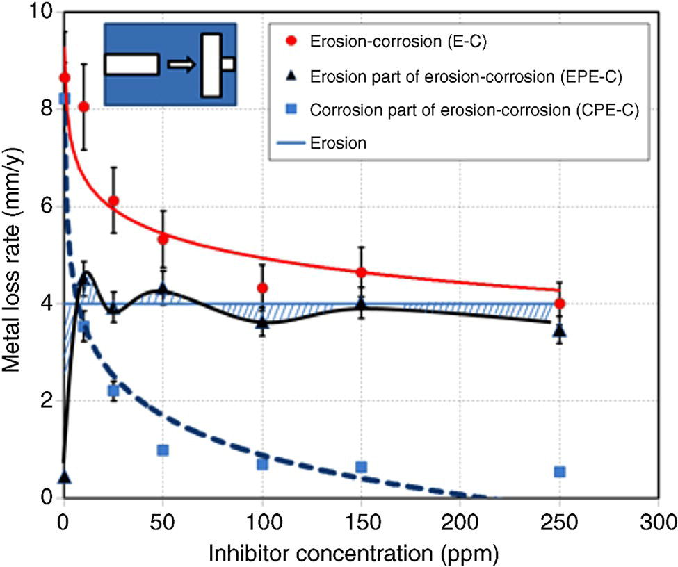
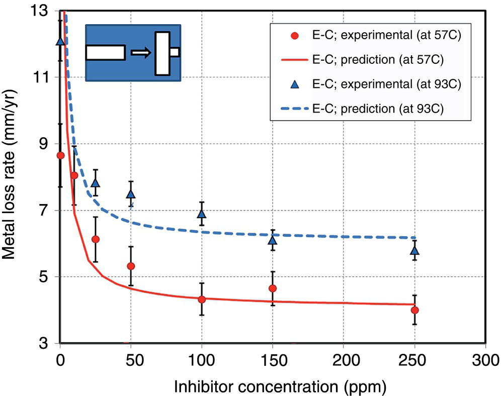
61.7 Summary and Conclusions
Acknowledgments
References
Notes
Erosion–Corrosion in Oil and Gas Pipelines
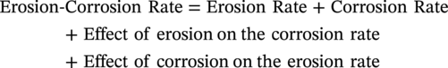


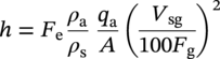
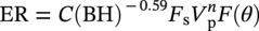

(61.10)
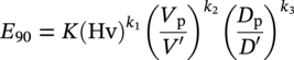

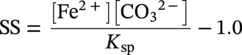
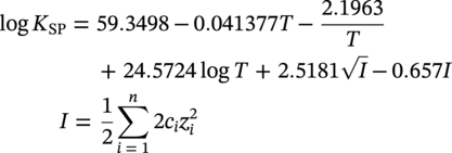
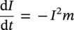
(61.16)