Brian N. Leis B N Leis Consultant, Inc., Worthington, OH, USA Prior to the mid-1960s, most pipeline operators considered it unlikely that a natural soil environment would initiate stress corrosion cracking (SCC) on line-pipe steels at typical service-induced temperatures, stresses, and cathodic potentials. That early thinking was proven wrong when a 24-in.-diameter Tennessee Gas Transmission Company (Tenneco) pipeline ruptured in a failure later attributed to SCC [1]. This rupture near Natchitoches, Louisiana, United States, on March 4, 1965, has been cited as the first evidence of failure of a pipeline due to external SCC [1]. Subsequent work in the 1990s supporting the development of Pipeline Research Council International (PRCI)’s high-pH SCC Protocol [2] located reference to a rupture on May 6, 1955, which occurred very near the site of the “first” SCC rupture [3]. Because its close proximity to the first rupture meant that the stressing, the steel, and the cracking environment would be similar, this reporting by the Research and Development group at the A O Smith Corporation (AOSC) was requested. Based on their reporting, the 1955 rupture was a “suspected stress-hydrogen failure.” Whereas the “first” SCC failure in 1965 had occurred about a mile downstream (D/S) of the Natchitoches compressor station, the 1955 rupture occurred much closer, at just 3000 ft (D/S) of that compressor station. In spite of the “suspected” cause reported by the AOSC, the imaging in what was a well-documented failure analysis for its era characterized features comparable to those of the 1965 rupture. This was visually evident in the cracking morphology viewed on the outside diameter (OD) of the pipe, and in metallographic cross-sections. Although reported as a “suspected” hydrogen-stress failure, their failure report listed and discussed features that they considered inconsistent with a hydrogen-related failure. These included: (1) very low steel hardness relative to what then was considered the threshold for hydrogen cracking, (2) significant ductility evident as a reduced-thickness pipe wall within the origin, and most critically, (3) the absence of chevrons and/or evidence of cleavage or quasi-cleavage fracture features. On this basis, the 1965 incident very likely was the second rupture to occur D/S of Tenneco’s compressor station near Natchitoches—the first having occurred about 10 years prior in 1955. Figure 53.1 reproduces the imaging at the origins of both failures, wherein it is apparent that their cracking morphology is similar on the pipe’s OD surface and in their metallographic x-sections. While not clear at the scale shown in Figure 53.1b, the micrographs for the 1965 rupture indicated that this cracking followed an intergranular (IG) path, which, while tight, was still visible in lightly etched views: that for the 1955 rupture appeared similar. The 1965 cracking was microscopically branched and showed directional changes in the cracking path that are evident macroscopically, which when examined at high magnification followed microstructural (grain) boundaries. The fracture surfaces for the 1965 rupture showed black thumbnail-shaped cracks, with similar features evident along one of the fracture surfaces reported for the 1955 rupture, which today are considered typical of both known forms of external pipeline SCC. The pipe’s OD surface for both ruptures as imaged in Figure 53.1a showed colonies of secondary cracking that today would be considered SCC. That cracking grew from an OD pipe surface that locally was free of significant pitting. Given these were the first recognizable instances of SCC on pipelines, as might be expected other pertinent aspects like the pH of disbond fluids were not detailed. That said, the cracking traits documented for these ruptures were typical of what today would be termed high-pH SCC. While prior to 1965 only two failures attributable to SCC were known, it was reported [4] that by the end of 1969 a total of 11 in-service failures had been attributed to SCC. During that same brief period, hydrostatic retesting and nondestructive technology (NDT) had revealed another 145 joints of pipe in which SCC was present, as either hydrotest failures1 or as still stable cracking. Those cracked pipes were found in 31 counties, in 14 states in the United States. As for the Natchitoches ruptures, 76% of this SCC was located within 5 miles D/S of a compressor station. Most lay on the lower quadrant of the pipe, being found in Grades from B to X-52, in a pipe made by several different producers. The affected lines had been in service between 7 and 27 years, with some lines being bare while others were coated—but all were subject to cathodic protection (CP) when this SCC was found. All such cracking occurred in pipes with typical mechanical properties, and normal compositions and typical microstructures. Figure 53.1 Images characterizing the traits of ruptures at Natchitoches a decade apart. (a) macro-views of the SCC on the OD surface, (b) cross-section micrographs. While most of the SCC failures between 1965 and 1969 shared the traits evident in Figure 53.1a, a few showed some features in cross-sections that were distinctly different from those of Figure 53.1b. Figure 53.2 presents macro-sections representative of this distinctly different cracking. While the cracking for most of the early SCC failures followed IG paths that were tight but open, the cracking in Figure 53.2a is not tight and shows heavily corroded flanks that, in some cases, are filled with compacted corrosion debris. Most of the early SCC failures showed branching along their length that was evident microscopically and grew from an OD surface that was largely free of pitting corrosion. In contrast, the few in-service ruptures that differed showed cracking that grew along rather straight segments and were branched at the macroscale as in Figure 53.2b, whereas most of the early SCC showed microbranching, which today is considered characteristic of IG SCC. The apparently different corrosion-broadened cracking that often was filled with compacted corrosion products was reported either as transgranular (TG) [6], or as involving a mix of some IG paths in otherwise TG cracking [7]. This TG and mixed cracking were observed to grow absent the microbranching that as noted above is characteristic of the IG SCC. Moreover, they tended to originate in clear evidence of corrosion pits on the OD pipe surface. For decades now, IG SCC has been associated with high-pH SCC, whereas TG SCC has been associated with what has been commonly termed near-neutral (NN) pH SCC. The groundwater pH if reported for the TG/mixed SCC that occurred on the bare but protected pipelines was noted as less than five. In contrast, when measured and reported, the pH under disbonds where IG cracking was present on the coated pipelines averaged 10.5 but ran as high as 12.3 [8]. This unusual TG to mixed cracking—as illustrated here, for example, in Figure 53.2—was reported only for pipelines that were initially bare but subject to CP later in service. Figure 53.2 Macro-cross-sections through cracking on bare but protected pipelines. (a) through secondary cracking found near a 1968 in-service rupture, (b) through the rupture path and secondary cracking found near a 1969 in-service failure. In 1969, the above-noted differences in cracking morphology between bare but later protected versus coated and protected pipelines had been recognized, as these different cases were clearly discriminated in the reporting of the many in-service ruptures and hydrotest failures that had occurred between 1965 and 1969 [4]. This potentially important distinction was lost by 1974 [8], as it was no longer noted or discussed in that or subsequent reporting. This is evident, for example, in the observation that the titles of figures detailing field cracking discriminated between images as bare versus coated pipe in 1969, whereas just 5 years later, this distinction was gone. This distinction between what can be corrosion-related SCC—whose traits are associated today with NN-pH SCC—and the failures more typical of high-pH SCC sets the stage for what follows later in this chapter and in Chapter 54. Recognizing the complexity of the factors controlling SCC that becomes evident as this chapter unfolds, it could take a book to address the scope of what has been learned since the mid-1960s. That said, this or any chapter must focus on just part of this complexity. This chapter opens with a laboratory-focused historical perspective concerning external axial SCC on pipelines and then adapts that historical perspective and insights since as the basis to quantify the cracking response for in-service pipelines. Based on the technical foundation of that laboratory work, it develops the framework to adapt those details as the means to assess the cracking response in field applications. Accordingly, results are presented that track the cracking response as a function of temperature and potential, doing so for the initiation and growth of shallow cracking and thereafter for cracking with depths sufficient to be characterized by fracture mechanics (FM) (hereafter termed macrocracks). Coupled with a criterion for the transition from shallow cracking to macrocracking, the laboratory data quantifies the average cracking speed (ACS) for each of the stages that comprise the “bathtub curve,” which has been adopted by some as representative of the in-service response of SCC over the life of a pipeline. Given the history of external SCC on pipelines this chapter begins considering high-pH SCC, and then transitions to briefly consider NN-pH SCC. This chapter outlines and discusses sparsely available archival data as the basis to quantify the factors controlling high-pH SCC. It then analyzes and trends those data leading to (1) cracking thresholds and speeds during initiation and early SCC growth, and thereafter does the same in regard to macrocrack growth. Changes in cracking speed are tracked as a function of depth specific to the steels involved, the pipeline’s operational parameters (stress, potential, and temperature), and the conditions along its right-of-way (RoW). These laboratory results are then used to quantify cracking thresholds and cracking speeds for both crack initiation and growth, which then calibrate each of the stages in the “bathtub life curve” for SCC in field applications. Physically measured field crack depths and their corresponding times in service are then compared to cracking speeds quantified by data from field digs and failure analyses. Confidence in the practical utility of the approach derives from its consistency with field cracking speeds for pipe steels considered highly susceptible versus those resistant to SCC. The traits of NN-pH SCC are introduced next for both initiation and growth in a brief section that discriminates between NN-pH and high-pH SCC—with a view to broaden the utility of the work presented specific to high-pH SCC. The ensuing discussion considers the cracking speeds presented in contrast to the guidance on cracking speed drawn from reporting by CEPA and UKOPA, and in association with ASME Code B31.8S. Finally, some disconnects between integrity assessment and in-line inspection (ILI) technology are discussed. Fessler circa 1976 gathered and trended discharge temperatures for 21 of the early service and hydrotest failures attributed to SCC [10]. Although some data pairs whose cracking traits were different from that for most of the early SCC incidents had been included, his work established a conclusive tie between the incidence of SCC and temperature for high-pH SCC. In the years that followed, Parkins worked his summer leave from the University of Newcastle upon Tyne at Battelle’s Columbus Laboratory. During that time, he likewise characterized the role of temperature and potential, and like Fessler and his colleagues also considered the role and nature of the cracking environment [10–12], and the steels involved. It was usual then to consider SCC as the synergistic consequence of stresses coupled with environment acting on a backdrop of a steel whose composition and microstructure rendered it susceptible to SCC in that environment. A review concerning SCC indicates that this remains the case [13]. The experimental work by Fessler and Parkins made use of smooth (un-notched/uncracked) samples subject to service-like stressing conditions,3 for which the testing was done in a concentrated electrolyte designed to simulate, yet still accelerate, crack initiation in the field environments then found associated with SCC. They also used typical precracked or notched samples to simulate crack growth under field conditions. As thresholds for initiation and growth were common with most cracking mechanisms, Fessler working with Barlo created a novel tapered tension (TT) test specimen [14] that was designed to quantify the role of the stressing conditions on crack nucleation and early growth. Fessler working with Parkins also considered crack-growth thresholds using samples based on FM concepts. Studies of the field (in-service) cracking environments (see footnote 3) led to the use of a concentrated cracking environment, which since has been referred to as the standard (high-pH) cracking environment. This “standard environment” comprised an aqueous one-normal (1N) sodium carbonate (Na2CO3)—one-normal (1N) sodium bicarbonate (NaHCO3) solution. As it was a concentrated solution relative to the field conditions, the cracking process in these laboratory tests was accelerated relative to the field cracking. As becomes evident shortly, significant further acceleration was achieved by testing at the potential that maximized the cracking speed for the steel involved, which for carbon steel pipes often was close to −650 mV SCE. Still, further acceleration was achieved by testing at an elevated temperature, with most such experiments being done at 75 °C (~167 °F). References [10–12] underlie Figures 53.3–53.5, which trend results from selected tests among those embedded in this early but comprehensive database. These figures illustrate the significant role of temperature and electrochemical potential based on testing specific to smooth (un-notched/uncracked) specimens. This testing used specimens cut from steel that had been removed from pipes involved in the initial in-service failures, as well as from related hydrotest failures. Accordingly, the steels used in this testing had proven susceptibility to a more dilute carbonate–bicarbonate electrolyte, which when field measured typically had a pH of ~9, or higher [8]. Prior to understanding the role of temperature as an accelerating factor, some compressor discharge temperatures upstream (U/S) of the failures approached 80 °C (176 °F), with even higher temperatures occasionally reported. Thus, the test temperature adopted for most of the standard testing in this context was a reasonable upper-bound to in-service temperature levels for the early field and hydrotest failures. Figure 53.3 Dependence of SCC crack-initiation speed as a function of temperature. (Adapted from [10].) Figure 53.4 Failure incidence reduction affected by reduced discharge temperature. (Adapted from [10].) Figure 53.5 Average crack speed versus potential for high-pH SCC of X52 line pipe steel. (Adapted from [10].) The role of temperature in the incidence of cracking alluded to earlier led to laboratory studies concerning the effect of temperature on cracking speed. Figure 53.3, adapted from Reference [10], illustrates the effect of temperature on the cracking speed4 during the initiation of SCC based on testing smooth steel samples in the concentrated carbonate–bicarbonate environment, at the optimal potential for cracking, which as noted above is about −650 mV SCE. The y-axis in Figure 53.3 is the ACS, which on the left margin is shown on a linear scale while on the right margin, it is shown on a logarithmic scale, both as a function of decreasing temperature5 shown on the x-axis. The lower x-axis is shown as inverse temperature relative to the Kelvin scale, while the upper axis presents the corresponding outcome specific to the Fahrenheit scale. These data indicate that decreasing the temperature results in a sharp initial decrease in the cracking speed, after which the sensitivity to temperature diminishes. In turn, a decreased cracking speed decreases the extent of cracking and the occurrence of deeper cracking, which leads to a reduced incidence of cracking and should permit longer reinspection intervals. Figure 53.4 illustrates the significance of the exponential dependence of crack speed on temperature, which is evident in the laboratory data of Figure 53.3. It shows the decreasing incidence of SCC as a function of the discharge temperature. These trends have been determined specific to curve-fits to experience-based cracking incidence as a function of the distance D/S of a compressor discharge relative to its discharge temperature. The y-axis in this figure shows the reduction in incidence as a result of decreasing the discharge temperature by the amount indicated on the x-axis. Data and predicted trends are included there for gas discharge at a temperature of 130 and 110 °F. The predictive trend shown as the solid line represents a simpler model that accounts only for the role of temperature. In contrast, that shown by the dashed line considers the role of temperature, and also addresses differences in the range of cracking potentials, which as becomes evident shortly also depends on temperature. Of these, the latter is most relevant in typical pipeline applications. Regardless of which predictive model is used, the key observation is that decreasing the discharge temperature significantly reduces the incidence of high-pH SCC failures. As expected, the amount of this reduction depends on the initial discharge temperature. It is evident here that reducing the discharge temperature by 40 °F cuts the failure incidence by more than 80%. Since the role of temperature was understood, changes have been made in the compression ratio, or after-coolers were added as needed, such that compressor discharge temperatures have since been reduced significantly. In considering the role of temperature regarding SCC initiation and growth reference has been made to testing at the “optimum potential” for SCC. Such was the case for the data characterizing the role of temperature reported in References [10–12]. Those same references considered other factors then thought to control the susceptibility to SCC, including potential. Figure 53.5 quantifies the effect of potential on the cracking speed as a function of the temperature used for each set of tests. All tests were done in the standard concentrated cracking environment (1N carbonate–1N bicarbonate solution) at a range of temperatures from 68 to 194 °F (20–90 °C). This range of temperatures was selected because it spanned what had been found for field (in-service) SCC failures. The trends shown in Figure 53.5 indicate that the same trend developed for each temperature. For each temperature, the ACS grew from a very low value, which in Figure 53.5 originates at a speed of 10−8 mm/s or less along the x-axis, after which the speed rapidly increased to a maximum value at a more negative potential, and then decayed rapidly to a very low speed as the potential continued to become more negative. As expected in view of Figure 53.3, the maximum cracking speed increased for each set of tests as their test temperature increased. As such, the cracking speed for shallow cracks shows a coupled dependence on temperature and potential. As noted earlier, this testing made use of smooth specimens sampled from pipes that had been removed as part of reparations made following the early in-service failures and/or hydrotest failures. On this basis, it can be said that the steels used had proven susceptibility to a more dilute carbonate–bicarbonate solution that when field-measured showed a pH the order of 9 or more. As evident in Figure 53.5, the trends developed for those steels showed that the higher cracking speeds occurred within a very narrow range of potentials at a given test temperature. The increase to or decrease from that maximum speed also occurred over a narrow range of potentials. These trends show that the cracking speed swings by a factor of 100 or more within a shift of just ~50 mV SCE, the extent to which depends somewhat on temperature. It follows that pipelines can be maintained at CP levels that will avoid IG SCC while also minimizing external corrosion at or below levels that typically have been adopted for that purpose (for example, −850 mV CSE or about −770 mV SCE).6 These data also showed that concern for CP levels that fall marginally below −850 mV CSE was less of an issue at temperatures below ~130 °F (55 °C). Finally, these data indicated that operating at potential levels outside the narrow range for SCC reduced the cracking speed by a factor of 100 or more as compared to the speed developed at the optimum potential that was imposed in most laboratory testing. In this context, the cracking speeds reported along the y-axis in Figure 53.3 could be reduced by a factor of 100 or more simply by maintaining CP levels close to the appropriate potential. The reason that cracking develops over a narrow range of potentials at a given temperature as evident in the potential trends shown in Figure 53.5 becomes apparent from consideration of the slow and fast sweep polarization curves shown in Figure 53.6a. These sweeps are representative of typical X52 line-pipe steels that were produced into the late 1960s, with similar trends also evident for the X60/X65 grades produced in that era. This testing was done in the standard concentrated electrolyte at a temperature of 75 °C (167 °F), with the sweeps made at a rate of one volt/minute (considered fast) and 20 mV/min (considered slow). Figure 53.6 Aspects of active passive cracking of X52 line-pipe steel. (a) current density versus potential. It is apparent from Figure 53.6a that potentials over which line-pipe steels are susceptible to high-pH SCC are bounded above by “anodic protection.” This state reflects the protective film that forms at a speed fast enough to prevent anodic dissolution at sites where new (electrochemically reactive) surface forms. Susceptibility to high-pH SCC is also bounded at lower potentials. This state reflects potentials for which the speed of bulk corrosion exceeds that for anodic dissolution confined within the grain boundaries. Potentiodynamic scans are useful to isolate this range of susceptible potentials because their trends indicate potentials at which a large difference in current density reflects high anodic activity under film-free conditions. Such conditions drive anodic dissolution at a high speed at film-free sites, whereas for other potentials, the speed of dissolution diminishes and films form, or general corrosion occurs. Such response indicates that in addition to the role of stress, the IG SCC process is also strain-rate dependent. Clear evidence of this strain-rate dependence follows in Figure 53.6b. Figure 53.6b, based on constant extension rate (CER) testing, indicates that there is a range of strain rates over which IG SCC can be sustained, with its maximum cracking speed developing at strain rates between ~10−5 and ~10−6 s−1 for testing of this X52 in the standard environment at the optimal potential and 75 °C (~167 °F). As for the effects of potential, this figure indicates differences in cracking speed as a function of strain rate that approach and conceptually exceed a factor of 100. It is apparent from Figure 53.6b that at lower strain rates, below ~5 × 10⁻⁹ s−1, SCC gives way to anodic protection, but depending on the local circumstances, corrosion could develop. In contrast, at higher strain rates, above ~2 × 10⁻⁵ s−1, SCC occurs slower than other cracking mechanisms, like stable tearing, which leads to diminishing SCC speeds. These results indicate a clear role for mechanics in quantifying the role of strain and its rate in assessing SCC cracking speeds, whether during initiation and early growth or later during propagation. Successful modeling of high-pH SCC, whose predictions were validated by direct comparisons with laboratory-measured cracking density and initiation thresholds [19, 20], was contingent on this strain-rate dependence, along with the other known controlling factors, such as potential and temperature. High-pH IG cracking of the exterior surface of a pipeline or the surface of a TT test specimen initiates on and grows into that surface by an “active-passive” mechanism [11, 12]. This mechanism underlies models of SCC that, for example, have been termed “film-rupture” [21] and “slip-dissolution” [22], with several variants based on similar schemes. All reflect service loadings that expose “bare” (i.e., electrochemically reactive) surface, which leads to crack advance by anodic dissolution focused within a grain boundary (GB) or similar interface. As the term “slip-dissolution” implies, this bare surface results from slip and the incompatible displacements it causes—wherein slip is the micro-mechanism of plastic flow. The occurrence of microplastic flow in a nominally elastic pipeline begs the question: If pipelines operate at stresses nominally well below the 0.5% yield stress (i.e., at design factors that run down from 0.80), then what is the source of this microplastic flow? One plausible source of slip (microplastic flow) follows from inspection of the hoop-stress-strain response for most any line-pipe steel, with several such curves sourced from Reference [23] being illustrated in Figure 53.7. These flattened-strap full-range hoop stress-strain curves are typical of the response for Grades from A25 up through X65 early in the era of their production. The scale of the x-axis is expanded in Figure 53.7b to values just beyond yield (defined here at a total strain of 0.5%) to illustrate this response at service-like strains. Figure 53.7b also shows trends indicating the usual elastic modulus for steel, as well as the 0.2% strain offset strain and 0.5% total strain. Bounds are also included to indicate the fractions of elastic and plastic strain, which comprise the 0.5% total strain—of which the plastic component reflects the cumulative slip that could create bare (reactive) surfaces. Figure 53.7b clearly indicates that microplastic strains develop at stresses well below the specified minimum yield strength (SMYS), which in turn could promote an electrochemically reactive surface on the OD surface of a pipeline at typical service stresses. In contrast, stress-strain curves developed in ring-tensile testing, which occurs free of the Bauschinger effect [24] that develops in flattened specimens, show little evidence of preyield plasticity [25]. Accordingly, the pre-yield plasticity evident in Figure 53.7 is unlikely to develop a reactive “bare” surface on an operating pipeline. Preyield microplasticity has, however, been demonstrated experimentally free of the Bauschinger effect in research involving a Fe-3Si steel [26] which in that work was observed at nominal stresses as low as 40–60% of SMYS. Specific to line-pipe steels, step changes in electrochemical activity have been shown in measurements of the current demand in tests of axial samples loaded elastically in tension [27]. That current demand reflects the creation of bare reactive surface triggered by the onset of microplasticity at similar nominal stresses, which in related work has been shown to depend on the prior plastic history of that steel. Figure 53.7 Stress-strain curves for a range of Grades from A25 to X65. (a) full-range response, (b) response up through yield. Microplasticity at stresses well below the nominal yield has been termed a “free-surface” effect, being so-named because flow with a component normal to a surface is unrestrained [19, 20]. As this effect reflects the absence of restraint to flow normal to the free-surface its effect must diminish as just nucleated SCC grows deeper, and restraint to slip develops due to the surrounding grains, which occurs within a depth of a few grains. Its effect also diminishes with growth along the surface that carries the just-initiated cracking outside the bounds of the originating grains that were favorably oriented for slip. In this context, the ACS in a TT test is expected to slow quickly as the cracking grows to a depth of a few grains. The viability of this free-surface effect and its influence on cracking will be evaluated in the next section, which considers cracking data developed in TT tests. The trends in Figure 53.6b and the discussion concerning Figure 53.7b indicate that if the loadings acting on a pipeline (pressure and any secondary loads) affect the onset of microplasticity at rates of straining consistent with active-passive cracking, then IG SCC becomes possible. In this context, the local stressing and its rate are among the determining factors for the speed of IG cracking. The stresses induced in that context couple with the effects of temperature and potential to determine the cracking speed specific to the local conditions. Cracking speeds for the isolated effects of temperature have been quantified for crack initiation and early growth for smooth samples by the data presented in Figure 53.3. Cracking speeds for the effect of potential at a range of constant temperatures have been quantified in Figure 53.5. It remains to quantify: These aspects are considered in the next several subsections. A test that suitably quantifies SCC initiation and early growth in smooth specimens must consider the factors known to affect differences in the ACS of SCC initiation and early growth as it occurs on pipelines. Thus, the test must provide native pipe surfaces; as surface residual stresses might exist, as might microstructural factors like decarburization or naturally occurring microstress raisers (e.g., oxides, pits, etc.). It also should address concerns such as anisotropy in the microstructure and resistance properties. The TT test specimen [14] alluded to earlier can provide a native pipe surface and is well suited for this purpose as it leads to similar thresholds in terms of diminishing cracking depth and diminishing cracking incidence. The drawback of the TT test is that to avoid prestrain effects due to the flattening of a hoop-aligned sample, the test sample adopted was aligned longitudinally. For present purposes, this is not a major issue. External SCC on pipelines has been a problem for reasons related to their age, their coatings, the metallurgy of their line-pipe steels, and other factors involving their RoW, construction, and climate. Taken together, these reasons have led to SCC being most problematic for conventionally produced Grades up to about X65. This class of steels generally does not show strong anisotropic microstructures and properties [28], so the longitudinal alignment of the TT test specimen is less a concern. Finally, because the initiation threshold stress developed by this test varies with the proportional limit taken as the 0.5% yield stress [29], its outcome would be slightly conservative in applications involving cold-expanded pipe. Managing SCC was a consideration when ASME B31.8S was being developed. Figure 53.8 presents the TT test data that was the background to aspects of that guidance [30], which here has been supplemented by additional data and reformatted. The y-axis presents the average depth (of the three deepest cracks) for cracking that was developing in susceptible steel. The x-axis presents the corresponding local stress in a TT test, normalized by the value of the 0.5% yield stress (AYS) for the steel. This normalized stress was used because prior testing [29], as well as modeling [19, 20], have indicated that it was effective in consolidating data for IG SCC. The progression of the IG SCC shown in Figure 53.8 has been benchmarked relative to arbitrary but representative depths for GB etching [20], and what were considered cracks [30–32]. The value of the threshold stress corresponding to the crack-depth benchmark lies between ~72% (or 37.4 ksi (258 MPa)) and ~85% of the yield stress (or 44.2 ksi (305 MPa)), which for this steel was close to and so taken at SMYS. Because the all-heat-average (AHA) 0.5% yield stress determined from material test reports must statistically exceed SMYS for a pipe order, the threshold stress inferred from Figure 53.8 for a pipe order would be scaled up relative to that shown here. For example, the ratio of the AHA yield stress to SMYS determined for about 50 X52 pipelines indicated that its value historically was ~17% larger than SMYS [33]. It follows that the crack-depth-based AHA threshold for X52 steels could run as high as 1.17 × 44.2 ksi or 51.7 ksi (i.e., almost the SMYS). This observation conflicts with reality—as an in-service IG SCC rupture had occurred at about 70% SMYS on the pipeline that this steel was sampled from. This observation suggests that for some steels the usual crack-depth criterion adopted to define the TT test threshold for SCC could be nonconservative, at least if based on 7-day or shorter tests. Figure 53.8 High-pH SCC threshold for typical X52 pipe steel. (Adapted from [30].) Although for decades a 7-day TT test has been used to quantify stress thresholds for crack growth from initially crack-free surfaces [32], longer-term TT, and related testing has shown that their outcomes depended on the test’s duration [34]. First, it has been noted that longer-term exposures to the cracking environment promoted continued but much slower GB etching beyond 7 days. As long as GB etching continued, IG growth at slower speeds was conceptually plausible. Second and practically far more relevant, longer-term TT testing had caused continued but slower crack growth well beyond 7 days [34]. (While an increase in the test duration affects a decrease in the ACS, the decrement in the ACS was beyond that effect for these longer-term tests.) It follows that the threshold stress for longer-term high-pH SCC can fall below that determined using a 7-day TT test. Taken together, the above observations indicate that the threshold stress for initiation should, in practice, be defined by the lower-bound value determined relative to GB etching, rather than crack depth, and that such testing should be continued long enough to establish a predictive trend in the cracking speed such that a lower bound to the threshold stress for field cracking could be inferred based on such testing. Because aspects involving macrocrack growth are considered in the next subsection, suffice it here to consider the implications of a threshold based on GB etching rather than on crack depth in regard to initiation. Inspection of Figure 53.8 indicates that the trend for GB etching for these data indicates a long-term threshold in the order of ~60% of the yield stress, or 31.2 ksi (215 MPa). In this context, high-pH SCC could be anticipated on pipelines characterized by these data operating at design factors as low as 0.6. As other case-specific factors, like the presence of localized stress raisers and material inhomogeneities can affect initiation, high-pH SCC is plausible on pipelines operating at potentially much lower nominal stresses. Finally, consider the results of Figure 53.8 in light of the earlier discussion concerning the free-surface effect. Note in this context that thresholds begin to become evident in this figure at crack depths the order of ~0.004 in. (0.10 mm) [32], while the threshold associated with the onset of GB etching corresponds to a depth set at ~0.002 in. (0.05 mm) [20]. Given the grain size of many pre-1970s X52 line-pipe steels ranged from ASTM 7–9 (from 16 to 32 μm or 0.00041–0.00081 in.), the GB TT-test threshold would reflect cracking from 2½ to 5 grains deep. Such depths are fully consistent with the free-surface effect discussed in the prior subsection. The results of TT tests like that just presented also can be analyzed to determine the average speed of crack growth over the period of the test. Figure 53.9 trends values of the ACS for a series of TT tests [34]. While the X52 line-pipe steel involved differed from that considered in Figure 53.8, its susceptibility was similar to other steels that had failed in service. In addition to the usual 7-day TT tests, this series of tests developed cracking in tests that were interrupted after 2, 4, 7, 14, 30, or 60 days. As becomes evident, these tests and so this figure reflect the ACS for physically shallow cracking that initiated and grew from the surfaces of smooth TT specimens. Figure 53.9a presents the average crack speed determined for each of these tests on the y-axis as a function of test duration shown on the x-axis. The axis scales were chosen in view of the need to present data that spanned several orders of magnitude, which was dealt with by logarithmic scales. Note that data for the usual 7-day tests are grouped separately from the longer-term tests to make clear the difference in the best-fit trending that develops for these datasets. Figure 53.9a indicates that if this testing had been stopped after 7 days as usual, then the outcome of this work would be best-fit by an exponential decay, which is evident as the dotted trend. This exponential trend develops an excellent fit as R2 is 0.998. It is apparent on the basis of this trending that the projected value of the ACS decays asymptotically toward 0 well within 100 days. A much different outcome results when the datapoints for the usual 7-day tests are trended along with the datapoints that developed for the longer-duration tests. As Figure 53.9a shows, this longer-duration dataset fits a power law (PL), shown there as the dashed trend. The datapoints for the usual 7-day TT tests lie along this PL trend within a tight scatter band for all datapoints. This PL equation likewise provides an excellent fit for this full dataset, as R2 is 0.983. More importantly, it characterizes the continued cracking that initiates and grows over the longer term, and so can be used to quantify the cracking speed during crack initiation and early growth from a smooth surface. Denoting time in days by t, the ACS expressed in mm/sec has the form: Figure 53.9 High-pH SCC TT test average cracking speed for X52 line pipe steel at 75 °C (167 °F). (a) TT test data for up to 60-days duration, (b) trend in part a) extrapolated to 50 years. which has affected a high-quality fit as R2 > 0.983. Figure 53.9b presents the same six datapoints and PL curve-fit, except that here the scales of the axes were expanded to accommodate extrapolation of this PL trend for a period up through 50 years. Denoting time, t, in years, the ACS for these six increasingly longer-duration TT tests has not changed, but as different units were used, the constant in the best-fit trend and Equation (53.1a) differs from that in Figure 53.9a: As for the exponential fit for the short-term tests, the PL fit across all the data through the longer-term testing affects a high-quality fit (R2 > 0.960). In the light of experiments done with crevices, Fessler et al. [35] have concluded that results developed in regard to potentials maintained on pipe surfaces in the context of high-pH SCC “are not likely to be altered if they occur in a crevice, such as at a pipeline surface where coating disbondment has taken place.” On that basis results as in Figure 53.9 and in Figures 53.3 and 53.5 can be used to simulate field IG cracking under disbonds. Figure 53.9b includes a second y-axis that quantifies the ACS on a linear basis, and involves changes in the units used. This leads to a shift in the locations of the TT test datapoints relative to the x– and y-axes as compared to Figure 53.9a. Although these test data characterize just one X52 line-pipe steel, results developed for a variety of other Grades from X42 up to X52 and X60 pipe indicate little difference in the outcome of the TT test if the stress is normalized relative to the AYS, as had been recognized decades ago [29]. In that context, the linear scale in Figure 53.9b indicates that ACS data gathered over a period up to 60 days span values that range from a maximum (near Faradaic) value down to values approaching zero. While extrapolating from the 60-day short-term data up through 50 years seems extreme because the multiplier on time is in excess of 300, the corresponding change in the ACS is very small, decreasing from 0.0019 mm/year to near zero over that period. It follows that at least for these data, TT testing for about 60 days provided a viable basis to extrapolate the ACS over a timeline consistent with typical pipeline applications, which in turn suffices to quantify the initial shape of the bathtub curve. Equation (53.1) indicates that the ACS drops below ~1 mm/year (~0.04 in./year) within 47 days, whereas after about 9 months it has fallen to ~0.25 mm/year (~0.01 in./year). After about 13 years, it has fallen to 0.025 mm/year (~0.001 in./year), and to 0.025 mm/year (~ 0.0005 in./year) after ~30 years. Given the fundamental dependence of high-pH SCC cracking speed on temperature presented in Figure 53.3, these ACSs that reflect accelerated testing at 75 °C will decrease in practice to applications at 5 °C by a factor of about 24. It follows that the ACS of shallow high-pH SCC could at 5 °C fall to about 0.025 mm/year (~0.001 in./year) within a few years of a cluster’s initiation. Crack depths calculated on the basis of Equation (53.1) are correspondingly shallow in the short term, requiring years to achieve depths that would threaten pipeline integrity. Earlier, the trends in Figure 53.8 indicated that depths associated with the onset of GB etching beyond the threshold for cracking ranged from ~0.002 in. (0.05 mm) up through ~0.004 in. (0.10 mm), both of which were evident at higher stresses within 7 days. Analysis based on Equation (53.1) indicates that as the ACS decays rapidly, the growth into the depth slows. As this response was developed in steels whose ASTM grain size was about 7, which corresponds to a diameter the order of 0.001 in. (0.025 mm)—these TT-test ACS data are consistent with the effects of the free surface considered in the previous section. While this consistency between speed and depth could be coincidental, modeling of high-pH crack nucleation and early growth based on this free-surface effect has correctly simulated the influence of hydrotesting on susceptibility [5]. This included a discriminating series of blind TT tests wherein specimens that had been prestrained to exhaust their free-surface microplasticity were predicted to be absent cracking local to the zone of that influence, which was confirmed in subsequent TT-testing [20]. Such results support the utility of this concept in practice. Recognizing that Figure 53.9b and Equation (53.1) quantify crack initiation and early growth for high-pH SCC at 75 °C at the optimal potential for cracking, care must be taken to utilize values of the ACS specific to the temperature and potential conditions along the pipeline’s RoW when using such results to simulate bathtub curves up through the onset of macrocrack growth. Various precracked test geometries have been used to quantify the threshold and ACS for macrocrack propagation, which have been subjected to either bending or tensile loading. The stress field local to the crack tip in tension-loaded FM specimens becomes more intense as the crack depth increases. The same occurs in load-controlled geometries where bending occurs, wherein this stress field is further intensified because the neutral bending axis shifts toward the back-surface of the specimen as the crack grows. These crack tip stress fields are broadly quantified in textbooks and handbooks for physically “deep” cracks in FM test specimens.7 The conditions local to the crack tip dictate how the driving force for cracking is determined. The driving force for “deep” cracks for which the resulting plastic zone is physically small compared to the size of the crack and the specimen can be quantified by linear-elastic FM (LEFM). In contrast, when the plastic zone at the crack tip becomes large relative to the size of the crack and the specimen, nonlinear FM must be used. Provided that the FM aspects are appropriately addressed there should be little difference in regard to the type of sample used and/or the nature of the precrack or notch. A downside for much of the high-pH SCC data developed for line-pipe steels might be that the extent of the crack growth beyond the precrack or notch is limited—often to less than a millimeter. From a FM perspective this is not an issue, because FM defines the resulting crack depth as that of the crack growth added to the depth of the precrack or notch. UKOPA SCC guidance [38] and ASME SCC Guidance [39] developed in support of ASME B31.8S [40] both cite the work of Koch, Beavers, and Berry [41] as the basis to quantify the ACS in the framework of FM. These authors developed their data in the usual “standard environment.” Although the potential used in that testing was not reported, it can reasonably be assumed at −650 mV SCE, as this was usual for most of the laboratory testing done at Battelle in that era. Their matrix involved testing at three temperatures set at 125, 150, and 175 °F (~52, 66, and 79 °C) for 7 days or for 28 days. Their matrix was implemented selectively using cantilever beams in bending, and surface-cracked plates in tension. The precrack depths for their tests led to four values of the LEFM crack-driving force, which is denoted K and known as the stress intensity factor. Recognizing that limited crack advance occurred in their tests, their four initial values of K, which were bounded between 15 and 30 ksi-in½ (~16.5 and ~33 MPa-m½), changed little over the course of a given test. In total, 21 tests were completed for the cantilever geometry, which included 3 done over a period of 28 days, whereas just 8 were done for the surface-cracked plate, all for a period of 7 days. The results of the just-noted testing are replicated in Figure 53.10a, wherein the data is presented as done in Reference [] in a format typical of FM tests—that is, crack advance is shown on the y-axis as a function of the stress intensity factor, K, shown on the x-axis. Figure 53.10a presents crack advance for each of their 7-day cantilever-beam tests, for each of the three tests done at the temperatures noted above. The measured threshold for macrocrack propagation is also shown on the x-axis, as determined through their independent testing of this steel. That threshold reported at 14.7 ksi-in½ (~16.2 MPa-m½) is comparable to that reported for other line-pipe steels [42, 43], values for which commonly ran as high as 18 ksi-in½ (~19.8 MPa-m½) for early-chemistry X65 steels [43], with values also reported as low as ~13 ksi-in½ (~14.3 MPa-m½) and as high as 22 ksi-in½ (~24.2 MPa-m½) [43]. Figure 53.10 Crack propagation as a function of temperature for high-pH SCC in X52 steel. (a) cantilever-bending crack growth. (Adapted from [41, 42].) , (b) average speed versus temperature. Inspection of Figure 53.10a indicates that significant scatter plagues these data when presented in the format used by Koch et al. In the worst case, these results indicate speeds that differ by a factor of 60 on crack advance, which as all data shown reflect cracking over the same time period means the cracking speed likewise scatters by a factor of 60. While not illustrated herein, even after the crack advance data were averaged for each K-temperature combination, this significant scatter persisted in the format of this figure. Inspection of Figure 53.10a also indicates that in this format this dataset fails to show clear trends with K, and/or with temperature—which is unusual at least in regard to temperature. Although the scatter was very large when their data was parsed as they did in terms of the FM crack-driving force, K, inspection of the data points in the format of Figure 53.10a suggests that a much different, near-scatter-free picture might emerge if these data were parsed by temperature, independent of K—as such is often the case for SCC macrocrack growth. Figure 53.10b presents a reanalysis of this data wherein the pooled average crack speed (equally crack advance) determined on that basis is shown on the y-axis as a function of the test temperature on the x-axis. There, it is evident that this alternate format develops little to no scatter and leads to a clear strong exponential decay of the ACS with decreasing temperature. This figure presents the outcomes of the deeply notched cantilever-beam samples (as in Figure 53.10a) as the open-circle symbols, ○, and the dashed trends. In addition, the results developed for the surface cracked tensile samples (absent in Figure 53.10a) are included, being shown by the x symbols. Figure 53.10b indicates that this pooled data leads to a tight exponential fit for the cantilever test geometry for the three temperatures that were considered. It is further apparent that the results for the surface-cracked geometry lie on or close to the trend for the cantilever samples—which along with the absence of scatter in this framework further indicates that the role of temperature overrides that of K. Denoting the average cracking speed by ACS, and the temperature by T in °C, the resulting exponential fit for ACS in mm/s had the form: which led to a R2 statistic of 0.999, indicating an excellent fit. Thus, this curve-fitted trend provides a viable basis to quantify the effect of temperature on the ACS for this high-pH dataset. Because the role of temperature overrides that of K, this relationship can be used throughout macrocrack growth, without regard to K. This independence on K simplifies the analysis of the in-service macrocrack growth due to high-pH pipeline SCC. As expected in view of Figure 53.3, Figure 53.10b shows that temperature has a significant effect on the ACS measured using notched or precracked test specimens, whose response by their design reflects that of larger (longer, deeper) actively growing cracks in colonies of IG SCC. But, as evident in Figure 53.10b as the temperature falls below ~100 °F (38 °C) the trend through this experimental ACS data converges with the x-axis, reflecting very slow cracking speeds and the diminishing significance of temperature. As the ACS slows, other processes like corrosion can become dominant, which can blunt the crack tip. This can further diminish the cracking speed, and could promote dormancy. Crack tip blunting also occurs due to the stretch across a crack’s tip due to local plasticity, caused for example by a high-pressure hydrotest. In addition, the debris formed by corrosion, whose volume is larger than the volume of steel consumed, can compact within the crack as cracks get tighter toward their tips. In turn, that compacted debris can limit transport of the cracking environment to the crack tip. If blocked from the cracking environment, the SCC falls dormant. Independent of corrosion, as the cracking slows the factors that drive SCC, like the environment and local stresses, become less significant, with factors like microstructural and compositional differences of the steel overtaking their importance. This too could lead to dormancy, or activate an alternative cracking mechanism. Unfortunately, corrosion acting along the flanks of a crack can eradicate the path of crack propagation, destroying evidence of an IG or TG cracking path—which can confound understanding of the type of SCC involved. It follows that as cracking slows many factors contribute to its tendency to lie dormant. In closure to this discussion of macrocrack propagation speed, note that the data in Figure 53.10b provides the means to quantify the potentially significant change in the cracking speed upon reversing the flow direction for the segment of a pipeline that had previously run at higher temperatures. For example, consider a flow reversal of a pipeline that decreases the temperature over a line segment from ~122 °F (50 °C) to ~68 °F (20 °C). Substituting the Centigrade equivalents into the equation shown in Figure 53.10b indicates that this decrease in operating temperature affects more than a 50-fold decrease in the macrocrack ACS—leading to ~0.009 mm/year (~0.00034 in./year). This speed lies along the x-axis where inspection of Figure 53.10b shows the data trend is represented by a dotted line—in place of the dashed line that was used to fit the test data. Such slow speeds tend to dormancy, as other factors like corrosion and microstructural/compositional differences of the steel can affect the cracking speed much more than temperature. Bear in mind as well that at the other end of the line there is a corresponding increase in speed, such that the effects of line reversal require ongoing SCC management. The prior sections have presented laboratory test results that quantify high-pH SCC in terms of: This section couples the results of these test results as inputs to develop a criterion that quantifies the transition-crack-depth from the initiation and early growth process in a smooth specimen to that of the macrocrack growth as quantified in an FM specimen. Figure 53.11a presents a framework, common to these otherwise quite different cracking scenarios, that leads to a mutually consistent criterion for the transition between them. The y-axis in Figure 53.11 is the nominal (remote) stress. Nominal stress was used in Figure 53.8 to quantify the onset of cracking in smooth specimens, like the TT test. Nominal (remote) stress also affects the onset of cracking in FM specimens, through its role in quantifying the crack-driving force, K, at the onset of macrocrack growth, denoted hereafter KTHscc. The x-axis in Figure 53.11a is crack depth, which was determined for the smooth specimen data as evident in Figure 53.8, and also in regard to the FM data as shown in Figure 53.10a. As for the smooth surface data from the TT tests, the remote stress at the transition to macrocrack plotted on the y-axis is the nominal stress imposed on the FM sample corresponding to KTHscc. Values of K plotted in the format of Figure 53.11 lie along a straight line with a slope of minus ½, which is characteristic of LEFM. The corresponding crack length that pins the location of this line along the x-axis is specific to K as defined for the FM sample geometry used to measure KTHscc. Figure 53.11 Transition between smooth and FM specimen cracking response for X52 steel. (a) representative transition response, (b) plausible range of transition depths. It follows that the framework in Figure 53.11 couples the factors controlling the onset of cracking from smooth surfaces to that at crack tips in FM-cracked geometries. The transition between these test conditions is defined by the intersection between their respective trends, as evident in Figure 53.11. The first trend is shown in Figure 53.11a as the dashed horizontal line, which reflects the threshold stress specific to Figure 53.8, as it lies at a y-axis value equal to 60% of SMYS, or 31.2 ksi (~215 MPa). As outlined earlier, this trend quantifies the threshold for GB etching—and the onset of high-pH SCC on a smooth surface. Lesser values of this threshold stress reflect more susceptible steels. The second trend shown in Figure 53.11a lies at a slope of −½, through a point on that trend specific to the value of KTHscc shown in Figure 53.10a, which was 14.7 ksi-in0.5. Lesser values of KTHscc reflect more susceptible steels. As becomes evident shortly, the value of the transition depth can change significantly depending on the steel’s susceptibility to SCC. Key in this context for IG SCC is the observation that the values of both thresholds can strongly depend on the R-ratio [43] (R = minimum/maximum stress in the cycle). The intersection of the horizontal stress trend for cracking from a surface, with the inclined trend for the FM samples, defines a mutually consistent transition between these test types. This depth is denoted dTH, indicating it is the transition threshold between the response for cracks growing from a free-surface to that for macrocracks, whose response is quantified using FM geometries. As the trends that define dTH in Figure 53.11a are specific to SCC, this depth threshold should be denoted dTHscc to signify it is specific to SCC, versus fatigue or other such mechanism. Inspection of Figure 53.11a indicates this transition occurs at a depth of ~0.070 in. (1.78 mm) for the thresholds that underlie this figure. This transition crack depth, dTHscc, involves a crack size that is deeper than that associated with the TT test data, while also being shallower than that associated with KTHscc. As the following content is specific to SCC, suffice it hereafter to denote this threshold by dTH. In addition to trends that reflect SCC, a third vertical trend has been included in Figure 53.11a that indicates the depth often used by ILI vendors as the threshold for the detection/reporting of cracklike anomalies [44]. Note that for this set of threshold conditions, the threshold depth claimed for ILI crack detection lies at depths less than the transition to macrocrack growth—which means that if the ILI tools perform as claimed then they should be able to locate cracking whose size could pose a SCC-based threat to pipeline integrity for this pipe steel if exposed to conditions that initiate high-pH SCC. As indicated above, the transition depth, dTH, varies depending on the threshold values for the onset of cracking from surfaces and from crack tips. Values evident in Figure 53.8 for cracking from a surface trended from ~93% SMYS down to ~60% of SMYS, which in view of the data reported in Reference [26] could go much lower. Regarding KTHscc, the values cited commonly ran from 18 ksi-in½ (~19.8 MPa-m½) down to as low as 13 ksi-in½ (~14.3 MPa-m½) [43]. Figure 53.11b illustrates the bounding trends for this set of conditions in the format of Figure 53.11a, which in turn lead to bounds on the corresponding range in the values of dTH. It is apparent from this image that the values of this depth threshold can differ by a factor of 4.5,8 with an upper-bound (U-B) value at 0.140 in. (3.56 mm) and a lower-bound (L-B) at 0.031 in. (0.079 mm). This range indicates that the susceptibility to high-pH SCC varies appreciably, being more dependent on the threshold stress for smooth specimens than on that for macrocrack growth. In this context, the combination of conditions considered in Figure 53.11a (shown as the solid circular datapoint) lies toward the L-B of the range shown, indicating that this dataset reflects a rather susceptible steel. This outcome is consistent with the observation that this transition depth was developed for steel whose threshold for the onset of IG SCC represented a pipeline that had experienced an in-service failure due to high-pH SCC. Figures 53.2 through 53.11 have characterized the response of line-pipe steel subject to conditions that promoted high-pH SCC under laboratory conditions. The use of such data in field applications requires that the differences between the laboratory conditions promoting that cracking versus that in the field be accounted for. Figure 53.12 organizes the factors considered to control both forms of SCC under field circumstances circa 1997 [45], which although somewhat dated remains relevant today at the level of detail it presents. While it represents both forms of SCC, it does not discriminate between them. This topic is briefly considered later in this chapter. The reality in regard to Figure 53.12 is that in many ways it reflects the same five factors known since the 1970s [12, 13] as having a controlling influence on whether SCC would initiate, and how fast it would grow. That said, these factors have been expanded to address the transition from the laboratory to the field, as well as the realization that since the 1970s a second type of external pipeline SCC was identified. Circa the 1970s, these factors included electrochemical potential; temperature; environment; the steel and its susceptibility in the cracking environment; and the rate of strain and the nature of the stressing—particularly the value of the stress ratio, denoted R. In addition to work done to quantify cracking speed and field-loading effects, much of the research and understanding since the early years has focused on: (1) reversibility of the cracking environments [17, 46] and the role of hydrogen [15, 16]; (2) the implications of shallow cracks [36, 37]; (3) down-crack transport and the role of corrosion debris blocking down-crack access [47]; and the detection and sizing of cracks [48, 49]. As chapters could be devoted to such topics, the purpose here is to highlight the scope of such work, rather than detail its results. Each of the factors noted must be addressed in managing SCC in regard to field digs as well as reinspection intervals. They also must be considered in constructing Bathtub Curves to support those processes that are specific to the operating and RoW being considered. Key in this context are: (1) the mechanical effects of the pressure history, including hydrotesting; (2) changes to the pipe’s surface, such as pitting; (3) the time required to incubate the environment; and (4) the time required to degrade the coating thereby providing its access to the pipe’s surface. Curves with the general shape of a bathtub profile and reference to it as a bathtub curve were first used to characterize degradation and failure in electrical systems and have more broadly been applied to mechanical and other systems for more than seven decades [50]. Given that the Bathtub Curve concept has been in use for more than seven decades, it is not a surprise that this concept was considered plausible in applications involving field failures of pipelines subject to SCC beginning in the mid-1980s [51]. Figure 53.12 Factors affecting external SCC on pipelines. (Adapted from [45].) Bathtub curves historically have identified three stages of response [50] as shown schematically in Figure 53.13a. An initial decrease in survivability, often termed Stage I, was ascribed to the effects of infant mortality. It was coupled with the occasional chance failure that occurred throughout the useful life of a system, termed Stage II. As the infant mortality failures drew down, Stage II became dominant, representing the slow but continued occurrence of chance failures. As the system aged, the chance of failures gave way to a noticeable increase in failures due to degradation—often termed wear-out failures—which comprised Stage III. The SCC process lacks a direct analog to infant mortality, although it does show a rapid initial decline in cracking speed. That initial cracking response as well as the SCC process more generally involves the chance coupling of stress, environment, and susceptible microstructure over the useful life of a pipeline. Following the initial rapid decline in cracking speed initially analogous to Stage I in Figure 53.13a, the cracking speed slows significantly to a more or less steady speed—analogous to Stage II. Thereafter, the cracking speed increases in parallel to the degradation process that comprises Stage III in the schematic shown in Figure 53.13a. In view of the above, adapting the historic Bathtub concept to SCC for present purposes simply requires a change in (1) the metrics it represents; and (2) its three conceptual Stages, to make provision for “incubation.” In lieu of the incidence of failure over time, the y-axis of the SCC Bathtub Curve should quantify the progression of SCC in terms of cracking speed. Crack depth, d, normalized by the pipe’s wall thickness, t, likewise could be used. Given that both crack speed as well as crack depth vary with the progression of time, the passage of time remains a viable x-axis metric. The resulting SCC Bathtub curve is shown schematically in Figure 53.13b. Cracking speed rather than normalized crack depth has been adopted herein to track the progression of SCC for three reasons. First, the faster the ACS, the sooner failure occurs, which leads to a relative increase in the failure rate, analogous to failure incidence in Figure 53.13a. Second, an ACS could be quantified for most any situation provided that the time prior to failure and the crack depth at failure were known, as is the case for forensic work. Finally, speed could be quantified based on laboratory cracking data and used to simulate the Bathtub Curve as a function of time. The merit of ACS in this context is that forensic data can be directly compared to the outcome of the Bathtub curve to validate the methodology used to simulate it. Regarding incubation, laboratory testing is typically done under circumstances that initiate and grow SCC almost as the test begins. For example, laboratory TT test data typically show well-established cracking within 2 days [34]. Thus, the time required for incubation is minimal for laboratory data, and as such, has been considered implicit in Stage I of the laboratory schematic of Figure 53.13b. In contrast, prior to the onset of SCC in the field the cracking environment must form and gain direct access to the pipe wall, such that the coating also must degrade. In the field the time for incubation so defined is unique to each SCC cluster along a given pipeline. While in concept, a laboratory test could be done that quantified the three Stages shown in Figure 53.13b, laboratory testing typically has relied on short-term accelerated testing of either smooth specimens and/or notched or precracked specimens. Such tests have typically been done under some form of load control to simulate the effects of pressure within a pipeline. Likewise, in concept, a laboratory test could be developed that ran continuously through those three Stages. That said, those smooth and/or notched/precracked specimens typically have been terminated after a target test duration is achieved—often within several days, or in some cases a few weeks. Figure 53.13 Bathtub curve concepts and their adaption to laboratory SCC. (a) conceptual bathtub curve, (b) concepts adapted for laboratory SCC. It follows that the response developed in typical laboratory tests do not lead to a continuous dataset that if plotted would appear like that shown schematically in Figure 53.13b. Rather, smooth specimens, which have been terminated typically early within Stage I have been used, whose results lead initially to very high values of ACS that rapidly decay. When such data are plotted as was done in Figure 53.9b, the limited longer-term TT test data available show that initial rapid decay follows a PL trend, which leads to very low speeds within a few months, as was evident in Figure 53.9b. It follows the results of smooth-specimen tests capture the trends evident in both Stage I and Stage II—absent a clear distinction between these stages. Data developed in short-term accelerated testing of notched or precracked specimens show increasing rates as the cracks grow, which reflects the effect of the load-controlled remote stress as occurs in Stage III. Thus, taken together within a framework that consistently defines the transition between Stage II and Stage III, such results could be adapted to quantify a bathtub curve for SCC. Coupled with the trends in Figures 53.3, 53.5, and 53.10, a wide range of ACS values could be developed to simulate the circumstances that control field cracking. It remains to address “incubation” in this transition from laboratory to field cracking, in which incubation becomes Stage 0. Given that high-pH SCC had been characterized since the mid-1960s, it is not a surprise that the bathtub concept was first postulated for applications involving SCC in regard to IG cracking [51]. As the differences between IG and TG cracking mechanisms were recognized, a TG-specific Bathtub curve emerged in CEPA’s 2007 Handbook [52]. Figure 53.14a adapts Parkins’ initial high-pH schematic specific to the results presented earlier in Figures 53.8–53.11, whereas Figure 53.14b reflects the CEPA NN-pH schematic bathtub curve. Inspection of these figures indicates that schematically the response they characterize differs only in regard to Stage III. While the Bathtub concept was postulated for SCC applications close to 40 years ago, as yet the axes of plots like these have not been broadly quantified, based either on sound science and/or rooted in relevant empirical data. The source documents for Parkins’ and CEPA’s schematic bathtub curves do not state whether time was quantified on a linear scale, or a logarithmic scale. Because a log-time scale expands time early in the cracking process, and thereafter increasingly compresses time as cracking continues, absent insight to the timeline between these schematics it is difficult to compare directly Figure 53.14a and b. Suffice it to note that both show an initial decay in cracking speed that is followed by cracking that has slowed to a near-constant value. Thereafter, both show a rapid increase in cracking speed. The response during Stage I of Figure 53.14 is akin to that evident in Figure 53.9b, which as discussed previously can be represented for high-pH SCC by the PL form of Equation (53.1). Stage II comprises the period during which the speed decreases slowly in comparison to the rapid decline evident in Stage I. Also analogous to Figure 53.9b, this response is quantified by Equation (53.1), such that the first two stages of the SCC Bathtub Curve reflect cracking as it develops and grows from a smooth surface—herein represented by TT test data. Because the speed throughout Stages I and II can be represented by the same equation, the schematic distinction between them shown in Figure 53.14a is quantitatively moot. Figure 53.14 Schematic Bathtub Curves adapted for high-pH and NN-pH SCC. (a) for high-pH SCC, by Parkins. (After [51].), (b) for NN-pH SCC by CEPA. (Adapted from [52].) Whereas Stage II preserves the historic format of the Bathtub Curve and is moot quantitatively, it is practically and conceptually critical in that dTH marks the end of Stage II. This follows from its definition within the framework of Figure 53.11, wherein the value of dTH was defined as the intersection of the threshold trends developed for initiation and early growth and for macrocrack propagation. In that context, the end of Stage II signifies the transition from cracking controlled by the free surface as in a TT test sample to macrocracking growth as in a FM-test sample. As noted above, the transition to Stage III reflects a shift to cracking at a well-defined crack tip, which significantly differs from that for growth from a smooth surface. Accordingly, beyond this transition, the response is quantified relative to the macrocrack behavior detailed earlier in regard to Figure 53.10. Consistent with previous work [43, 53], this growth was independent of the value of the stress intensity and quantified only in regard to temperature for high-pH SCC by Equation (53.2). Recent work has cited the just noted results, and similar work that quantified such cracking, which showed that the ACS also depended strongly with the potential, but less so on the pH and stressing conditions [54, 55]. Such results would facilitate adapting this approach across a broad range of field conditions. When the threshold crack depth, dTH, is exceeded, the ACS begins to increase. Figure 53.10a along with prior work [43, 53] indicates that this FM crack growth only occurs at values of K ≥ KTHscc. Inspection of Figure 53.11b indicates that for susceptible steels the values of dTH are the order of 0.030 in. (0.76 mm), which is small in comparison to the notch/precrack depths used in typical FM testing. At the lowest of the measured values of KTHscc noted earlier, the crack depth is the order of 1 mm for testing of X52 FM specimens at 72% of SMYS. The initial crack depths in the FM test samples considered in Figure 53.11b were already greater than the transition depth, such that the value of KTHscc could be shown coincident with dTH, as has been done in Figure 53.14a. The ACS at depths larger than dTH differs for high-pH SCC versus that for NN-pH SCC (e.g., [54, 55]), which underlies the essential difference in the trends shown in Figure 53.14a and b. Consistent with the active-passive nature of IG SCC, Figure 53.14a shows the cracking response rising first to and then across a Faradaic plateau and continuing beyond that at still faster speeds until failure. While the life fraction afforded to Stage III in this schematic is rather large, because the Faradaic plateau exists at a very high value of ACS, the time required to traverse this plateau could be relatively small in comparison to the overall serviceable life for a pipeline operating at worst-case temperatures and potentials. In contrast, because the mechanisms that underlie NN-pH SCC show traits similar to that of corrosion fatigue [56] the growth trend shown in Figure 53.14b rises gradually toward failure, and then increases sharply much like that for high-pH SCC. Assuming that the cracking remains stable as it grows through the wall, as this cracking deepens pressure-driven net-section collapse or fracture ensues. In ductile line-pipe steels, the cracking mechanism transitions to ductile tearing via micro-void nucleation, and its coalescence (MVNC), and the ACS increases until failure, as has been shown in this schematic. Failure for purposes of the simulated bathtub curves that follow reflects such stable through-wall cracking, leading to an axially stable crack that opens a leak path. Failure also could result in cracking that becomes axially unstable as the wall is breached. Discriminating between axially stable versus unstable cracking and leaks versus ruptures is complex [57], and so well beyond the present scope. Suffice it for present purposes to note that a leak occurs through axially stable features, whereas the term rupture reflects an axially unstable response.9 Equations (53.1) and (53.2)10 were combined with values of the depth threshold, dTH, considered representative of a highly susceptible steel and resistant steel based on the trends in Figure 53.11 to simulate bathtub curves for these extremes in resistance. The resulting bathtub curves are shown in Figure 53.15a and b, respectively. The value of dTH that underlies Figure 53.15a was taken at 0.76 mm (0.030 in.), which as noted earlier reflects a “highly susceptible” steel. In contrast, the value of dTH for Figure 53.5b was taken at 1.65 mm (0.065 in.), which earlier discussion of Figure 53.11 considered a “resistant” steel. Figure 53.15 Bathtub curves quantified for two bounding scenarios involving high-pH SCC. (a) highly susceptible steel, (b) resistant steel. The short-dash trends in Figure 53.15 reflect growth from the exterior surface of the pipeline for which the ACS is quantified by Equation (53.1). Cracking continues on that basis until a crack has formed with a depth equal to dTH. At depths deeper than dTH, the cracking transitions to FM control, which is shown as the longer-dash trends and quantified by Equation (53.2) as a function of the temperature. As noted earlier, the schematic in Figure 53.14a includes a reference to KTHscc. That said, because values of K ≥ KTHscc involve depths that exceed dTH, the value of KTHscc is not a factor in simulating these curves. In this context, dTH functions in this framework are analogous to that of KTHscc in other predictive schemes. As plotted, these simulations reflect almost immediate initiation, and so make no field-based allowance for incubation, which is considered following this Subsection. Once nucleated, SCC typically develops within a cluster of cracking that either continues to grow until failure ensues or the cracking goes dormant. Evidence of stop–start and/or dormant cracking has been observed in both the field [58] and laboratory [59]. Inspection of Figure 53.15 indicates that the majority of the service life for these near-worst-case operational circumstances is spent within Stage II, while that spent in Stage III is quite short. As the factors controlling SCC noted in Figure 53.12 became known, the informed pipeline operators responded. Discharge temperatures were reduced, and potential was controlled, which significantly increased the duration of Stage III. For example, inspection of Figure 53.10b indicates that a decrease in temperature from 75 °C (176 °F) down to 45 °C (113 °F) causes the duration of Stage III to increase by more than 50 times. The trend reported by Song et al. [54] indicates that a similar increase in life accrues to controlled potential. On this basis, in contrast to Figure 53.15, the time interval associated with Stage III could more than suffice to manage SCC reliant on inspection-based condition assessment. The practical utility of bathtub curves like those shown in Figure 53.15 is best assessed in reference to field-failure experience. Archival failure reporting indicates that the earliest amongst the IG SCC field failures known to the author [60] occurred within 7 years of its in-service date. Other pipelines constructed in that era have been found recently with very shallow (but likely dormant) high-pH SCC. Those lines operated initially under similar conditions and since have survived for more than 70 years without suffering failure due to IG SCC. Such results appear consistent with the lives evident in Figure 53.15 for the susceptible and resistant steels considered therein. Comparable data exist regarding two early IG SCC failures on an X52 pipeline constructed in 1950, which has suffered recurrent failures since. This line was one of four parallel lines constructed sequentially to meet the then-growing demand. All made use of X52 and used similar construction and coating practices, and all were supplied off a common manifold, so their operating histories were similar. All were laterally spaced as usual since the 1950s in a common RoW and were maintained similarly, so those aspects were also similar. Yet, while being similar in all ways, the line that suffered the two early failures has since experienced recurrent failures. Its response regarding the early failures appears consistent with the lives evident in Figure 53.15a for the susceptible steel considered therein. In contrast, the other three lines have operated without evidence of SCC, with their response being like that evident in Figure 53.15b for the resistant steel considered therein. It can be inferred in this context that different steels of the same Grade can embody different susceptibilities to IG SCC. Such differences in susceptibility exist at the scale of similar pipelines but are also evident in areas of cracking that lie under a common disbond adjacent to areas that remained crack-free. Such behavior is broadly illustrated in Chapter 54, which deals with the traits of SCC (see, for example, Figures 54.8, 54.9, 54.12, and 54.13). Unfortunately, as yet we have little definitive insight into why pipe surfaces that lie under a common disbond show areas free of IG SCC interspersed between active clusters of cracking. In summary, an inspection of Figure 53.15 indicates that the highly susceptible case considered in Figure 53.15a failed in just 3.4 years. When a few years are added for incubation, the time predicted for field failure is close to that of the earliest US rupture, which occurred within 7 years [60]. Likewise, the life predicted for the resistant steel is consistent with the survival of the many pipelines constructed in the 1940s and 1950s that remain in service in the US without evidence from IG SCC. On this basis, the lives simulated for the bounding cases involving a highly susceptible steel and a resistant steel (shown respectively in Figure 53.15a and b) are consistent with the range of cracking speeds and resulting service for these field data. In turn, it follows that the bounds on susceptibility represented in Figure 53.11b, which underlie these simulations, reasonably bracket the above-noted extremes in predicted life associated with IG SCC. It remains to consider the time required for the degradation of the coating, and thereafter the time required to form the cracking environment on the pipe wall within a disbond, which together were earlier termed incubation. By definition, the time to failure in the field is the sum of the time (1) for incubation and (2) for crack initiation and growth to failure. As such, laboratory and field data developed under comparable conditions could be analyzed to infer the incubation time. The simulations in Figure 53.15 considered the time for crack initiation and growth to failure—absent incubation based on TT and FM testing developed under conditions that reflect the cracking environments and operation characteristics of the early US field failures [8]. On that basis, the time required for incubation could be inferred by subtracting the shortest time predicted to initiate and grow cracks to failure for the susceptible steel. Inspection of Figure 53.15a indicates failure occurred in 3.95 years, such that the shortest incubation time would be inferred by subtracting 3.95 years from the commissioning date for the first US field failure—earlier noted to be 7 years. Incubation times could similarly be determined relative to the population of US SCC failures that occurred up through about the mid-1980s, by which time the research-based controls to manage IG SCC had been broadly published [12, 61]. The results developed on this basis are plotted as the data points in Figure 53.16a. It equally might be argued that the time for incubation could be estimated by subtracting the time to failure for the laboratory TT testing that occurs absent incubation from that same set of field failures. The results for that laboratory testing reproduced from Figure 53.9 are included for reference as the dashed line shown in Figure 53.16b. The x-datapoints in Figure 53.16a correspond to the reported failure lives after subtracting the 3.95-year period associated with crack initiation and growth based on the bathtub curve in Figure 53.15a. The fastest incubation time for this dataset develops for the shortest in-service period prior to failure, which as noted earlier was ~7 years. Allowing 3.95 years for initiation and growth leads to incubation after just 3.05 years, which is highlighted in the figure by the circled x. The best fit to this inferred incubation period leads to a PL, which, due to the use of a constant initiation and growth period, indicates that incubation time increases as the time to failure increases. Incubation time inferred relative to the time to failure in the laboratory is shown in Figure 53.16b as the dotted trend leads to a similar outcome, the results for which are plotted in Figure 53.16b as the + symbols. As for the inferred incubation times shown in Figure 53.16a, these inferred times are best-fit by a PL. Comparing the trends for incubation based on the worst-case predicted time for initiation and growth to failure (Figure 53.16a) with that for the laboratory TT tests (Figure 53.16b) indicates that both lead to comparable best-fit slopes. The PL fits of these trends indicate that the time for incubation is a constant fraction (~1/15) of the time spent initiating and growing the cracking. Such is plausible in that some of the factors that drive coating failure are also drivers for cracking. While the trends to this point support the use of the approach advanced to simulate the cracking behavior in the field, the field data considered to this point are limited, and tend to focus on shorter lives and higher values of the ACS. The next subsection broadens this field cracking database to remove this limitation on their scope. IG SCC that can be sized relative to its time history can be obtained from field digs where cutouts have been done to validate ILI runs or for other reasons, as well as from hot-tap coupons or from pipe segment cutouts in association with field failures. Crack profiles exposed at origins in field failures typically intersect multiple adjacent cracks. Likewise, serial sectioning of cracks in clusters typically intersects multiple cracks, occasionally 10 or more, depending on the size of the sample considered. The downside for most commercially developed sources of data is that proprietary or legal considerations often constrain what can be made public. Figure 53.16 Trends involving early high-pH field failures and inferred incubation times. (a) inferred incubation times, (b) TT-test data versus early field failures. IG cracking data obtained from eight sources [62–69] suffice for present purposes, the results for which are presented in Figure 53.17. While the sizes and grades of the line pipe and the timeframe can be reported for these datasets, in most cases the operators cannot be identified, and the reporting is proprietary. These archived IG service failures spanned lives from 6.6 years up through 55 years, and involved nominal diameters from 6 to 30 in. (152–762 mm), for which 39 ≤ D/t ≤ 104, with all being X52 save for one involving X65. In two cases, the pipe was bare but protected. The pipe for the remainder was protected and coated, most commonly with coal tar. The x-axis in Figure 53.17 plots the number of years since the pipeline commissioning date until it failed or to when the cracked pipe ring or sample was removed from service, hereafter, the “life.” The y-axis plots the ACS determined by dividing the crack depth by the life. The bathtub schematics (Figure 53.14) indicate that this ACS reflects brief periods of cracking at quite high speeds as the cracking initiates and again as macrocrack growth ensues. As these brief periods at high speeds are short lived, the speed during Stage II tends to dominate the ACS over the total life to failure. Such is the case even for the highly susceptible steel (Figure 53.15a), in spite of its relatively short predicted life. On this basis, the values of the ACS so determined can be considered representative during the lifespan of typical field cracking. Figure 53.17a and b compare the ACSs predicted based on Equation (53.1) with values of the ACS determined for nine large datasets. Figure 53.17a plots results for four of the nine datasets in a format analogous to Figure 53.9b, wherein the ACS was shown on a linear scale while the life was shown on a logarithmic scale. Because the laboratory work involved short-term testing whereas field cracking occurred over decades, the bulk of the field data lie compressed into the lower right corner of this figure. Figure 53.17b expands a portion of the x-axis and reformats the y-axis of Figure 53.17a using logarithmic scales to expand the content of interest. It continues the use of the data legend from part a), and broadens that scope in regard to five additional datasets. The dataset, labeled “origins” in Figure 53.17a, reflects the ACS through failure for the deepest crack within the origins of in-service ruptures and leaks [69]. This dataset has been identified in Figure 53.17 by the + symbols. For cracking that led to a rupture, their crack depths were sized via software referenced to digitally captured images that contained the origin’s profile, doing so after the image had been magnified locally by at least 5 times. This same practice was used for leaks that had been opened following a soak in liquid nitrogen (LN). The depths for a second dataset were measured in a similar manner. This dataset differed from the first in that it comprised cracks that lay to either side of and near the origin of the leak path or the rupture. Depths for short isolated cracks were found within this dataset, which occasionally exceeded that for the deepest crack found within the origin. This second dataset is represented in Figure 53.17 by the filled-square symbols [65, 68, 69]. Figure 53.17 Comparison of TT-test-predicted and field-observed IG SCC speeds. (a) scales as in Figure 9b, (b) axes expanded to show the details, (c) histogram characterizing the crack populations shown in part (a). The third dataset comprised the remainder of the data, all of which were sized on serial sections, typically at 5X or better, with the measurements made using a digitally reported traveling stage [62–64, 66, 67]. These data differ from the prior two datasets as this IG cracking lay in joints located far from the origin or in cutouts removed during field digs unrelated to a failure. As for the second dataset, deep isolated cracking was occasionally evident in this group. With reference to Figure 53.17b, the data representing the deepest cracking within failure origins (the cross-symbols) lie toward the upper bound for these ACS data. Cracking near the origins of ruptures or nearby along the rupture path and/or leak paths (represented by the solid-box symbols) generally falls marginally below the deepest cracking (i.e., that typically at the origins). Finally, values of the ACS gathered at sites remote to or unrelated to origins (the remaining symbols) fall at lower speeds. In this format, it appears that the field failures represent the leading edge of a still-growing population of cracks. If indeed these service failures lie along the leading edge of a still-growing crack population, then unless such cracking can be proven dormant, these trends indicate that the shallower secondary IG cracks must be managed, otherwise, the incidence of field failures will continue to increase over time. Figure 53.17c reformats the dataset shown in part b) as a histogram relative to d/t (normalized crack depth), rather than relative to the ACS—except that this histogram excludes the results for the in-service failures. The occurrences that comprise this histogram are represented by the solid vertical bars as a function of d/t. The line connecting the filled symbols quantifies the cumulative sum of these occurrences. The y-axis on the left margin is the number of occurrences for each of the d/t bins shown on the x-axis, whereas the value on the right margin is the accumulating sum of those occurrences as a function of d/t. In this format, the deepest cracks lie toward the right margin, whereas the shallowest cracks lie toward the left margin. At d/t = 1.0 (right margin), a crack is through wall; whereas at d/t = 0 (left margin), a crack has yet to initiate. Crack depths that have led to in-service failures lie within the box inset in the lower right corner of this histogram. Inspection of Figure 53.17c indicates that for resistant steels and the wall thicknesses involved the transition depth threshold, dTH, lies at d/t ≥ 0.43, such that deeper cracking could transition to macrocrack growth potentially leading to failure. For susceptible steels and the wall thicknesses involved the transition depth threshold for this population lies at d/t ≥ 0.11, such that deeper cracking could transition to macrocrack growth potentially leading to failure. In summary, parsing this comprehensive crack population indicates that typically the deepest among these cracks lay within the origins, while the shallowest were found well remote to or unrelated to the origins, whereas the in-service ruptures comprised the leading edge of this population. It follows that, unless such shallower cracking can be proven dormant, such populations of IG SCC must be managed to avoid recurrent failures. This trending is consistent with the recurrent failures found on some pipelines into the late 1970s in the US, whereafter insights from the research of the 1970s led to the use of aftercoolers and reduced compression ratios, and better control of the CP. Additional insight into the nature of that and other SCC crack growth can be found in Chapter 54, along with more detailed analyses of field cracking. Several observations and practical takeaways follow in regard to the trends evident in Figure 53.17, which provided graphical evidence that supports/validates the concepts and the predictive scheme that underlies the bathtub curves of Figure 53.15, as follows: Except for generic discussion of the factors that control SCC in regard to Figure 53.12, this chapter has focused on IG (high-pH) SCC. That said, much of what has been presented specific to high-pH SCC is conceptually applicable to NN-pH SCC—provided that the key differences between these forms of SCC that affect susceptibility and the cracking kinetics are accounted for, and the differences affected by the transported product like pressure cycling are addressed, along with those specific to the RoW. While previously evident as discussed regarding Figure 53.2, the traits now considered typical of NN-pH SCC became broadly evident about the late 1980s, following study of the first of the several ruptures that prompted the NEB Hearing concerning SCC in Canada [9]. Insight into the differences between these forms of SCC can be gleaned from work that began with the first of those failures, and that done in preparation for that NEB Hearing. As that work progressed, it became apparent that the features evident in the “bare pipe” failures circa the late 1960s were again evident in what was considered a new form of SCC. As discriminating data became available, the differences between these two forms of SCC were contrasted and documented, which occurred for the most part in the years prior to, and following the turn of the millennium [9, 15–18, 39, 52, 70–72]). Insight into the differences associated with the transported products affected by the pressure history likewise can be gleaned from the literature, as summarized for example by Fessler et al., last in 2008 [39, 56], and by others more recently [54, 55]. Table 53.1 summarizes guidance concerning the traits that discriminate these two forms of SCC in the format that they were initially documented circa 1996, with many nuances and insights added based on the extensive field, laboratory, and related analyses done since. While small segments of this tabulation continue in use from their prior reporting, Table 53.1 has changed significantly versus its original content. The tabular format of its forerunner circa the late 1990s has been retained, with columns now parsing the differences versus similarities between the two forms of SCC.11 Similar traits are evident in the content that cross-cuts the columns, whereas the differences lie within columns specific to each form of SCC. Like its forerunner, its content was developed by trending empirical observations now made in regard to many hundreds of field digs involving both forms of SCC. At the high level dictated by the tabular summary format, each of the “Parameters” (listed in the leftmost column) repeated here from the first tabulation remain relevant today, but with modifications. Many other layers of parameters have been added, which reflect the broader experience and insight available today. While the prior trending circa the 1990s reflected SCC as it was emerging in Canada up through the NEB Hearing, the content of Table 53.1 now reflects the experience and insight gathered in many countries spread across most continents.12 While it is difficult to address in this compact format, where feasible this tabulation indicates how some of the trends have evolved over time. Table 53.1 Guidance Concerning the Two Accepted Forms of SCC in Summary a Many among these parameters can combine synergistically, with somewhat different outcomes. b “Near-neutral” covers pH values from ~ 4.5 to 8.4 (the lower limit reflects the observation that aggressive corrosion occurs faster than SCC, whereas the upper-limit reflects the equilibrium pH for the CO2H2O system). c The intent of “high-stress ratio” is to discriminate between SCC and corrosion fatigue, which occurs at moderate and lower stress ratios by an environmentally effected alternating slip mechanism. d Because SCC requires direct access of the aqueous cracking environment to the pipe steel, as occurs under disbonded coatings, cracking below well-bonded fusion-bonded epoxy (FBE) and other modern liquid coatings likely involve another mechanism, like a hydrogen-related cracking mechanism. e The pH must be read within minutes to an hour of its sampling—the bounds cited in part reflect the solubility curves for the predominant species in the CO2H2O system, and field experience. f Potentials cited are field-specific values referenced to a copper-copper sulfate (CCS) electrode—courtesy of Mr. J. E. Marr. g Alternating current voltage gradient (ACVG) surveys can be a useful complement to other methods to identify coating issues, like disbonds. h Report the nominal direction of the cracking and the lengths for individual and interlinked (visually coalesced) cracks measured and recorded in reference to their locations on quality digital MPI imaging—report depths where shallow and practical for sizing by the usual grinding/buffing and related procedures; report the deeper features after sizing by advanced (preferred) or conventional UT in the hands of field-experience-proven inspectors. For present purposes, the compare–contrast framework of Table 53.1 has focused on field cracking susceptibility and kinetics over the useful life of a pipeline. That field behavior is characterized by a robust laboratory database that quantifies high-pH SCC from initiation and early growth up through macrocrack growth. In contrast, such work involving NN-pH SCC has focused on macrocrack growth—with little work done regarding cracking response and speeds for initiation and early growth, which constrains developing Bathtub curves for this form of SCC. Suffice it here to identify the traits that directly affect the limited set of metrics in Table 53.1 that affect cracking susceptibility and kinetics, which largely fall within the heavy-dashed box overlaid on this tabulation. Key metrics in this context include the cracking environment (temperature, local potential, electrolyte, species), none of which are a surprise based on the content presented in regard to the high-pH type of SCC. The stress-component of SCC continues as a key metric, which as the tabulation shows is common to both forms of SCC. Microstructure continues as the background that the stress and environment components of SCC develop on, such that it too has been shared across both forms of SCC. The remaining parameters either influence or reflect the effects of the parameters within the heavy-dashed box, or they are consequent to their controlling effects. Relative to the guidance developed in preparing for the 1996 NEB SCC Hearing [9] and in developing the PRCI high-pH SCC susceptibility-ranking protocol [2], the current framework improves discrimination, particularly in regard to location, coating, and environment. Important in this context is the inference circa the mid-1990s that the cracking environments for both forms of SCC were seasonally reversible [46], which since has been shown possible in a laboratory setting [17, 18], depending on the temperature and the electrolyte balance between the key environmental species. Central to this is the strong inverse dependence of CO2 solubility on temperature. A seasonal influence on the cracking environment also could derive from seasonally dependent periods of heavy rain, which in some areas can be followed by periods of draught—leading to seasonal wet–dry cycles. This could alter the presence of various species and their groundwater concentrations, as well as the local values of the CP and pH. Differences such as those outlined above indicate that susceptibility to high-pH SCC requires satisfying many parameters, whereas these metrics suggest that it can be easier to satisfy the metrics for cracking via NN-pH SCC, which appears to be influenced by corrosion, and a less restrictive set of controlling factors. In Chapter 54, NN-pH and high-pH SCC are further contrasted in greater detail. Earlier discussion in regard to Figures 53.1–53.10 considered ACSs based on laboratory data for which the tests were accelerated by way of extremes in temperature and potential as compared to levels typical of service today. Related discussion in the context of the simulated bathtub curves and since provides insight into when and where SCC might be anticipated to occur based on operational and other factors. This section considers cracking speeds as they occur under field conditions, first in regard to industry guidance, and thereafter in regard to when and where SCC might be anticipated to occur. As the industry guidance generally has not been specific to the form of cracking, this section continues that practice. Industry guidance provides benchmarks for average SCC speeds,13 although this often is done without clear reference to the source. UKOPA [38] has cited an “upper-bound” speed of 0.3 mm/year (0.012 in./year). CEPA over the years has cited a range of speeds [52, 72, 73]. Specific to NN-pH SCC [73], they repeated a previously stated speed of 0.6 mm/year (0.024 in./year). Elsewhere in their guidance they also note a maximum speed of 0.88 mm/year (0.035 in./year), which they indicated was based on field simulation testing. Finally, Fessler et al. [39] in work aligned with ASME B31.8S [40] have provided a “representative” speed of 0.3 mm/year (0.012 in./year). It is apparent in regard to the shape of the schematic bathtub curves (see Figure 53.14) that at least for high-pH SCC the ACS in service varies depending on the Stage involved. The exception to this is Stage II, wherein the ACS decreases very slowly, doing so at values much slower than cited in the above-noted speed guidance. Significant in this context—the bathtub curves shown in Figure 53.15 and the field data included as its validation in Figure 53.17 both indicate that the field cracking speed during Stage II is about two orders of magnitude (i.e., 100 times) slower than that suggested by the industry guidance. This begs the question: what ACS characterizes my pipeline’s SCC? While a one-size-fits-all ACS, as cited in the Guidance must be conservative, the values cited could be caveated specific to the circumstances they quantify. Alternatively, they could be discussed within the broader state of knowledge that underlies them. In that same vein, such Guidance could be updated as new insights become available. Finally, in view of Figures 53.11 and 53.15, it is apparent that speeds such as those noted in the Guidance are relevant only as the cracking reaches depths for the onset of macrocrack growth. That said, at least for high-pH SCC the ACS is strongly dependent on temperature, slowing significantly as the discharge temperature and other aspects are brought under control. The first tabulation of susceptibility criteria based on field metrics emerged from the extensive trending of the circumstances associated with service and hydrotest failures, and related field digs, in work done under the auspices of CEPA prior to the NEB SCC Hearing [74]. By 2002, a broader set of criteria emerged under the auspices of the ASME, initially in the context of high-pH SCC [75]. The high-pH criteria circa 2002 indicated that such cracking could be anticipated if: (1) the pipeline was more than 10 years old; (2) was not externally coated with FBE; (3) was operated at a stress level above 60% SMYS; (4) at a maximum temperature above 38 °C (~100 °F); and (5) was within 20 miles (32 km) of a compressor discharge. By 2010 these criteria had morphed slightly in reference to NN-pH SCC [40], namely, more than 10 years old; not externally coated with FBE; and operated at a stress level above 60% SMYS.14 This set of industry-based susceptibility criteria has remained unchanged since they were introduced, which occurred more than a decade ago in regard to NN-pH SCC and more than two decades ago for high-pH SCC. Whereas evidence existed as these criteria were being formulated that SCC had occurred on lines then operated at stresses less than 60% of SMYS, the documentation was limited, such that SCC was not considered likely at stresses below 60%. Likewise, data existed then that showed high-pH SCC had occurred on lines then with discharge temperatures well below 38 °C (~100 °F), and at distances far greater than 20 miles (32 km) from a compressor discharge [10, 76]. But, again uncertain details and the weight of the evidence then available supported the criteria adopted circa 2000. It is apparent from failures and field digs trended since, which in part underlie the traits summarized in Table 53.1, that SCC has occurred at lower nominal stresses and temperatures, and been found beyond the scope noted in the ASME Guidance. The point to be emphasized is that the criteria advanced over the years as Industry Guidance are nothing more than guidance. Under no circumstance should such criteria be considered bounding rules of thumb. Pipe segments operating under conditions that fall outside the just-noted criteria can and have failed due to SCC. Equally, thousands of miles of pipelines have operated within these criteria that have remained free of SCC. That said, these criteria might best be implemented first in regard to the worst-case combinations of these criteria amongst the pipe segments being assessed. If following a thorough review no cracking is found, and (1) SCC has not been evident in the past, and (2) sites involving disbonded coatings and a range of potential environmental conditions were considered, then one might reasonably conclude that SCC is unlikely an issue. In contrast, if there is a history of SCC, and/or SCC was found for the worst-case scenario, then prudence dictates broadening the search—if possible guided by insight from aboveground surveys in addition to the usual close-interval practice. Finally, the use of FBE does not ensure that SCC or SCC-like forms of environmentally assisted cracking won’t occur. Not all mill-applied or field applied FBE coatings have been correctly applied on an appropriately prepared still clean surface. FBE coatings have failed and disbonds have been reported. That said, blindly using FBE as the opt-out regarding the threat posed by SCC could be problematic over the long term. By the turn of the new Millennium both the oil and gas (O&G) industry and the Regulator had recognized the benefits that might accrue to inspection-based condition monitoring and integrity assessment. Because initially this activity was largely focused within the United States, the convergence of inspection to quantify conditions with integrity assessment to establish safe serviceable pipelines is considered herein relative to that framework and its history. The O&G Industry had been proactively developing technology relevant to integrity and condition assessment in the years leading up to and following the new Millennium. Alternative integrity verification (AIV), which relied on inspection-based condition assessment, was pioneered in work funded in 1995 by the Pipeline Research Council International (PRCI), which then was focused on offshore pipelines. Its development was reported in considerable detail by 1997 [77], and summarized for the industry in 2000 [78]. To assure its success in its high-consequence offshore applications, its practice as developed included consideration of the viability of both the inspection and assessment capabilities, and the specifications needed to affect it, with a view to minimize the uncertainties in its application. The 2000 revision of DNV-OS-F101 [79] titled Submarine Pipeline Systems was the first codified integrity management (IM) framework published that adopted an inspection-based assessment approach. In this same timeframe peer-review drafts of the API Standard 1160 [80] and the supplement to the ASME Code B31.8 (denoted B31.8S) [40] were being circulated for comment and approval, each of which incorporated inspection-based condition assessment. Work to develop standards directed at effective inline and other inspection practices also had been underway since 1996 [81]. In parallel, the US Federal Regulator was drafting notices of pending rulemakings whose provisions included inspection-based condition assessment, as follows next. In the years just prior to the turn of the new millennium, the US Regulatory framework was undergoing changes and related developments. This began in the mid-1990s, driven in the US by the Accountable Pipeline Safety and Partnership Act of 1996 [82]. A Risk Management Demonstration Program stemmed from that, with a view to assess whether the principles and processes of risk management might provide an effective alternative regulatory framework for the US pipeline industry. Although the use of such methods has been permitted in the US for some time, as yet they have not been as broadly adopted nor codified to the extent that has occurred elsewhere, or been adopted by some Regulators [83]. By early April of 2000 a press release foreshadowed pending Regulatory changes, stating that “this summer we will see a major overhaul of our safety standards” [84]. That same year the US Office of the Inspector General [85] (OIG) stated that the “regulator must expand their research and development activities to improve the capabilities of tools referred to as smart pigs.” The OIG’s comments specifically noted applications involving cracks and select other features. While the Vendors have continued to make improvements, the Government has from time to time questioned whether the available ILI crack-detection (CD) tools can (1) reliably detect cracklike features, discriminate between feature types and locations, and (2) size them with adequate accuracy and precision [86]. While improvements focused on reducing the number of false positives reduce the cost of the inspection process, the downside is that they do not always reduce the risk profile, and in that context have little influence on integrity. In contrast, false negatives can lead to features that remain latent in-service after the IM, the larger of which have the potential to cause failures. This section considers IM in regard to more effectively coupling the inspection and assessment technologies—which prior to 2000 and in some ways since have continued to develop independent of the interface that exists between them within the current AIV/inspection-based IM process. Improving the interface between inspection and assessment technologies in applications involving SCC involves the coupled understanding of the detection and sizing problems posed by SCC, and the use of consensus terms and definitions. Consider first the role of definitions. Insight into potential semantics concerns can be gained by reference to the definition of a crack in the Pipeline Operators Forum (POF) ILI Specification [81].16 The POF defines a crack as a planar, two-dimensional feature with a high length to width ratio, a sharp root radius, and a possible displacement (separation) < 0.1 mm (0.0039 in.) across the crack surfaces. To an engineer, this seems appropriate. In contrast, a lawyer seeking to discredit an FM-based fit-for-service analysis associated with broadly gapped secondary stress-corrosion cracking, like that illustrated in Figure 53.18, could by reference to the large gap and this definition argue that those still intact features were not cracks. Likewise, it might be argued that the features that opened leading to failure also were not cracks, thereby discrediting a FM (crack)-based safety assessment. A stretch?—Perhaps! The point simply is that definitions worded by engineers consistent with their typical applications could equally be reinterpreted to suit other interests. Figure 53.18 Broadly gapped short deep secondary SCC near an in-service rupture origin. In total, the POF Specification defines eight additional terms relevant to quantifying SCC for the purposes of IM. In alphabetic sequence these are cluster, colony, cracklike, detection threshold, interaction, measurement threshold, reporting threshold, and sizing accuracy. Of the eight terms noted, cluster, colony, crack, and interaction reflect the potential complexity of the cracking due to SCC as compared to an isolated cracklike feature. The many faces shown by SCC pose a challenge to those writing definitions that characterize its traits. As evident from the wide gap across the crack faces evident in Figure 53.18, the current definition of a crack is unnecessarily restrictive—a sharp crack tip and long compared to its width might suffice. Yet, this remains ambiguous regarding “sharp”—and “long” compared to its “width.” The POF specification has appropriately defined interaction as “two or more adjacent anomalies …. that …. weaken the pipeline more than either would individually.” A cluster is defined as “two or more adjacent anomalies …. that may interact to weaken the pipeline more than either would individually,” which differs subtly from the definition of interaction. Others might define a cluster more simply, as closely spaced SCC found under a common disbond. Finally, a colony is defined in the Standard as a “grouping of stress corrosion cracks (or clusters?) occurring in groups of a few to thousands of cracks within a relative confined area.” Others might define a colony as a group of clusters located under a common disbond. Care should be taken to avoid wording that excludes SCC that has initiated and grown as one isolated cracklike feature—because such features have grown through wall and caused leaks. In contrast, the many short tight cracks often found within some clusters often tend to stop growing due to stress-shielding, potentially becoming dormant and so benign. From an inspection perspective, the traits of SCC are typically quantified in regard to detection and sizing requirements—whereas the IM analyst seeks sizing outcomes from the inspection that can be input directly to a severity assessment of the SCC. Crack lengths and depths and their in-plane spacing are primary inputs to such assessments. Because the threat posed by SCC is very dependent on axial coalescence17 between adjacent cracks, a technically sound assessment of SCC seeks crack-specific characterization of a colony that quantifies the crack spacings as well as the dimensions of the larger cracklike features that lie in close proximity. Crack detection and sizing to provide such inputs are currently commercially available from ILI tools that utilize liquid-coupled sensors based on ultrasonic technology (UT), or those that use a variation on UT that relies on dry-coupled sensors implemented by means of electro-magnetic acoustic technology (EMAT). The UT CD tools typically report pipe-body features on smooth pipe walls that are ~25 mm (~1 in.) in length, with a depth equal to or in excess of 1 mm (0.039 in.). Features are reported in regard to their location and are characterized/illustrated in terms of A-Scans, B-Scans, and C-Scans. Features detected are described by a feature identifier (ID), and quantified in terms of their boxed in-plane size (length and width), with the depth reported in mm increments that exceed the reporting threshold. That said, individual feature lengths can be identified to the extent they were called. Figure 53.19 In-ditch NDE to size depth and digitally document lengths and spacings. (a) depths via sequential phased-array ultrasonic testing (PAUT), (b) in-plane image of cracking. The EMAT CD tools likewise typically report pipe-body features specific to smooth pipe walls for features that are 40–50 mm (~1.57–1.96 in.) in length at depths in excess of 1 mm (0.039 in.). Along with location, the features are described by an ID, for example, cracklike or linear anomaly. Reportable features are characterized by cluster images akin to B- and C-Scans and in other graphical formats, and quantified in terms of their depth, typically as a whole-number fraction of the wall thickness, with the in-plane feature size boxed in regard to length and width similar to that noted for UT CD tools. Because CD ILI runs currently provide a map of the potential SCC hotspots, the SCC IM process relies on the tool run to detect all features that pose an immediate or near-term threat. As run quality can vary, and uncertainty remains that all features of concern are detected and reliably sized, following the ILI run direct examination (DE) is done at select digs. This DE provides inputs to validate the run, and to characterize/quantify the cracking within apparent hotspots. Given that commercially available ILI services do not claim to detect all features that would pose a threat, the potential consequences of false negatives should be addressed by supplemental practices. The digs and the DE should, at a minimum, follow the best of the industry guidance (e.g., CEPA [52, 72, 73] or NACE18 SP0204 [87]), and where useful capitalize on the insight provided by terrain models [88]. Dig sites based on those suggested by the vendor should be considered, as should independently selected sites. The in-ditch nondestructive examination (NDE) should make use of the most advanced UT and allied technologies, and be done by inspectors with truth-test proven track records. Depths should be sequentially sized along the major features, and high-resolution digital in-plane imaging should be done to facilitate postinspection analysis of crack stability, such as that shown in Figure 53.19. Thereafter, image analysis can be used to determine crack lengths and spacings, and be used along with other inputs to quantify the failure pressure and to assess crack stability. There also is merit in collaborative discussions concerning the reported length of SCC features in regard to their sizing by ILI and in-ditch NDE as a function of the crack aspect ratio (crack length, L, divided by depth, d). While the depth is reported for an ILI run relative to the OD surface, the length from the run is logically sized relative to the detection threshold rather than at the pipe’s surface, as shown schematically in Figure 53.20a (after [81]). In contrast, the length can be directly sized based on in-ditch imaging, whereas the depth must be inferred from indirect measurements. The inability to compare like-for-like measurements can complicate depth-based run validation, and opens to uncertainty concerning the length to use in IM assessments. As indicated above, the crack depths, d, and the lengths, L, of each reportable feature along with their proximity to adjacent cracks determine which among their adjacent tips might coalesce, potentially leading to a rupture and its consequences. In that context CD tools should locate and size the reportable cracking and output the details necessary to support IM cluster-by-cluster with sufficient accuracy to identify which of the colonies should be dug on a prioritized basis. For pipelines wherein only a few small colonies are found, there is little need to prioritize because just a few digs might suffice. In contrast, for ILI runs that call anomalies across a large number of colonies the potential number of digs could be large. In such cases, cost-effective IM requires outputs from the ILI run that support ranking threat severity colony-by-colony—which can require more than the dimensions of boxed clusters and crack depths sized in coarse increments. Only then can a practical yet viable dig plan be developed and implemented. Thereafter, individual feature lengths as sized in the ditch, could be coupled with crack spacing and the sizes of the adjacent features to assess leak versus rupture and the failure pressures for specific clusters/colonies of SCC. Figure 53.20 Implications of crack length as characterized by ILI. (a) crack length (After POF Figure 2.9.), (b) L/d for two quite different coalesced cracks. The schematic shown in Figure 53.20a infers that crack lengths reported at the depth-detection threshold underestimate the actual crack depth. For features with lower aspect ratios, the length reported at the detection depth will reasonably reflect the actual length. While this disparity is tolerable at small crack aspect ratios, as this ratio increases the length at the reporting depth is increasingly undersized, leading to nonconservative predictions of the failure pressure, and leak versus rupture. Early work indicated that values of the aspect ratio for SCC ranged up from ~1.5, to values approaching 20 [89]. Coalesced cracking with aspect ratios toward the extremes of this interval are imaged, for example, in Figure 53.20b.19 Figure 53.21a trends values of the aspect ratio from recent work involving a much broader database of directly measured crack lengths and depths in geometrically similar pipelines.20 Inspection of this figure shows these data slightly extend the just-noted bounds, to values from about one to those approaching 25. It is apparent from Figure 53.21a that the aspect ratio is large for shallower cracking, and decreases as the cracks deepen. Whereas the very high aspect ratios occur for shallower cracking that does not pose an integrity threat, the significance of this nonconservative disparity has been evaluated relative to crack depths that have caused in-service SCC leaks and ruptures. Figure 53.21b indicates that such failures have occurred in SCC clusters in transmission pipelines whose depths were less than 40% of the wall thickness and that they have occurred frequently at depths approaching 60%. At such depths, L/D can be reasonably taken at five. Adopting an aspect ratio of 5 and a depth at 60% of the wall thickness relative to a nominal pipe wall of 0.360 in. (9.1 mm), then if the crack profiles were semielliptic the relative error in its length would be the order of 2%. While for idealized semielliptic shapes the error is small, crack shapes often appear like that evident in Figure 53.20b, wherein the crack tips do not intersect the pipe’s OD surface as occurs for semielliptic shapes. For the cracking shown in Figure 53.20b, the disparity in length now approaches 8%. For fracture-controlled failure and the lower-toughness levels typical of many of the early fracture-controlled SCC failures, the resulting error in failure pressure for the semielliptic shape is tolerable, as it is comparable to that in the crack length. Such is less the case for the cracking shown in Figure 53.20b. That said, given the rather short critical lengths for these lower-toughness steels, even a small error in length could be the difference between a leak versus a rupture. The upside is that by trending “big data” and using geometry the length quantified at the reporting depth could be reasonably “corrected” to offset this error. Moreover, by digging hotspot areas of cracking based on the ILI output the ensuing quantitative IM analysis of failure pressures and leak versus rupture could be referenced to in-ditch measurements. To the extent the in-ditch measurements of lengths and depths reflect reality, direct comparisons of the results of hydrotesting SCC in pups removed from service indicate that viable predictions of both the failure pressure and leak versus rupture can be achieved [57]. Figure 53.21 Trends in stress-corrosion cracking and failures as a function of d/t. (a) aspect ratio as a function of d/t. (Adapted from [90].) , (b) normalized L/d as a function of d/t. (Adapted from [90].) Thresholds have been introduced by the vendors for the tools and technologies used to detect, size, and report cracklike features. The POF currently defines three thresholds [81]: one specific to detection, a second to sizing, while the third deals with the minimum size that is reported following the tool run. Reporting thresholds on crack depth, d, and length, L, are evaluated in this subsection relative to directly measured crack depths and lengths developed for the several large populations of crack sizes reported in detail in the next chapter. The crack-depth reporting threshold is evaluated first across a range of normalized crack depths, denoted d/t, for five wall thicknesses. Those depths are then coupled with trends in the crack aspect ratio, L/d, ratio determined as a function of d/t to assess the viability of current crack-length reporting thresholds relative to the range of crack sizes that have caused in-service leaks and ruptures due to SCC. Finally, field inspection experience involving SCC is considered in terms of a unity plot for a recent-generation ILI CD tool run. Takeaways follow thereafter. First, crack depth, d, was determined for specific values of normalized depth, d/t, across a range of wall thicknesses, t, for which SCC has been problematic—notably from 0.250 to 0.500 in. (6.35 and 12.7 mm). This led to the crack depths for this range of wall thicknesses that are listed by column in Table 53.2. These depths were obtained simply by multiplying the value of d/t noted for each row by the wall thickness for each of the columns. Inspection of the tabulation indicates that this was done for values of d/t up to 80% of the pipe wall. Values of crack depth that fell below a 1 mm (0.039 in.) depth-reporting threshold have been shadowed in light grey. Review of Table 53.2 across the range of parameters considered indicates that cracks less than 10% of the wall thickness in the thinner wall pipes would go unreported for a 1 mm (0.039 in.) threshold. Except for the thinnest of the wall thicknesses considered, all cracks deeper than 15% of the wall thickness would be reported for this threshold. In view of this tabulation, the current 1 mm (0.039 in.) depth threshold culls out many of the otherwise benign features, such that the current depth reporting threshold avoids many nuisance digs, whereas it reports the deeper cracking. Figure 53.21a has trended values of the aspect ratio as a function of their corresponding crack depths normalized by their wall thickness, d/t, which provides a means to estimate the crack lengths that correspond to the depths listed in Table 53.2. Given the scatter evident in Figure 53.21a, which traces largely to differences in toughness, a high-percentile value of the aspect ratio for a given crack-depth interval determines a physically based near upper-bound estimate of the crack length over that interval, with a value targeting the 80th percentile aspect ratio adopted for present purposes. Figure 53.22 presents the resulting trend fitted to those smoothed 80th percentile values of the aspect ratio as a function of d/t. Table 53.2 Reported Versus Unreported Crack Depths as a Function of t and d/t Figure 53.22 Trend through the smoothed 80th percentile values of the aspect ratio versus d/t. The values of the aspect ratio trended as a function of the corresponding normalized crack depths in Figure 53.22 provide the means to estimate the crack lengths that correspond to the depths listed in Table 53.2. As noted above, the use of a high-percentile value of the aspect ratio leads to near-upper-bound estimates of crack length. Table 53.3, which presents the crack lengths determined for each of the depths listed in Table 53.2, has the same format as Table 53.2 except that two columns have been added along its left margin. The leftmost column lists the approximate range of the aspect ratio determined for the depth intervals considered in Table 53.2. The next column lists the smoothed values of the 80th percentile aspect ratios for each depth interval. Multiplying this aspect ratio by the depths listed in Table 53.1 leads to a near-upper-bound estimate of crack length for each of the depths and wall thicknesses considered in Table 53.2. As for Table 53.2, the crack lengths listed in Table 53.3 that fall below a 1-in. (25.4 mm) reporting threshold have been shadowed in light grey. A study of Table 53.3 indicates that a much different picture emerges as compared to that evident in Table 53.2. It is apparent that a 1-in. (25.4 mm) reporting length threshold broadly constrains reporting of cracks at depths ≤40% of the wall thickness, except for thicker walled pipelines. This reporting threshold is slightly less restrictive for depths up to 60% of the wall thickness, except for the thinner of the pipe walls considered. Even cracks with depths up to 80% of the wall thickness could go unreported in some commonly encountered wall thicknesses. Because the current UT length reporting threshold is more stringent relative to the longer threshold adopted for some EMAT tools, this picture is somewhat bleaker for those tools. The practical significance of the depths and lengths in Tables 53.2 and 53.3 becomes evident by reference to Figure 53.21b, which recall was based on physically measured crack depths and lengths for a range of crack sizes. As the symbol key in this figure indicates, these data were parsed as ruptures, leaks, and secondary cracks near leaks and ruptures, and as less consequential cracking. This figure indicated that in-service SCC leaks and ruptures have occurred at depths less than 60% of the wall thickness, all of which have occurred in pipelines whose wall thickness was less than 0.400 in. (10.2 mm). Note, too, that for most of these cases, the measured aspect ratios were less than those used to develop Table 53.3. Such is likewise the case for depths up to 80% for the thinnest of the pipes considered. Table 53.3 Reported Versus Unreported Crack Lengths as a Function of d/t and t It follows by this evaluation that the reporting of the axial cracklike anomalies whose sizes correspond to the shallower leaks and ruptures evident in Figure 53.22b could be constrained by the current length reporting threshold for UT CD tools—even more so for some EMAT tools. Because this conclusion reflects aspect ratios targeting its 80th percentile value, some similarly-sized cracks could be reported by virtue of their actual size exceeding the 80th percentile. Two factors condition this outcome. First, because the cumulative distributions of lengths and depths on pipelines are biased toward shorter, shallower cracking (cf. Figure 53.17c), the likelihood of detecting and reporting cracks is highest for shallower cracking—all else being equal. Equally important, the relative uncertainty of the 80th percentile value adopted for L/d is least for the shallow cracking. Inspection of Tables 53.2 and 53.3 in this context indicates that if detected the cracks that exceed the 80th percentile value most likely include: (1) the shallower but reportable depths whose lengths are close to reportable in Table 53.3, and (2) some of the much deeper features with near-reportable lengths. The next subsection considers this inference in light of a unity plot for an ILI run completed on a line that had experienced an in-service SCC rupture within the last 10 years, using a tool configured then much as it remains today. The unity plot shown in Figure 53.23 compares the depths reported in an EMAT tool run with those gathered via in-the-ditch NDE as the line was being remediated following its in-service rupture due to SCC. Although the pipe was ejected from the ditch consequent to its rupture, the gas did not ignite. The field digs done to validate the run made use of usual in-ditch NDE and related practices—follow-up physical crack sizes were not available. Figure 53.23 EMAT unity plot for a pipeline that had experienced an in-service SCC rupture. In total, more than 20 sites were daylighted and examined the results of which were used to refine the preliminary run report, after which the final report was issued. The line was then hydrotested to satisfy Regulatory requirements, which it survived without failure, after which service was reinstated. The results associated with the many initial digs are labeled “initial digs” in Figure 53.23. While the anomalies at these more than 20 sites were called “linear,” SCC was not found among them. Follow-up digs also were done at several sites a few years after the rupture. The outcomes of these subsequent digs also are shown in Figure 53.23 relative to their sizes as reported in the tool run, being labeled there “delayed digs.” As evident from the plot, SCC was confirmed at two of these delayed digs. Figure 53.23 indicates that the features reported tended to cluster toward shallower depths, with just a single point reported for a quite deep feature. This is as was anticipated above regarding the trends evident across Tables 53.2 and 53.3. While the trends evident in this EMAT unity plot are mirrored in a range of other unity plots, including those for UT runs, the plots in hand represent a small cross-section of what is available. That said, the results across 50 or more runs could be assembled for each NN- and high-pH cracking for each sizing technology as the basis to reassess the suitability of the current length reporting criteria. If that outcome continues to indicate the current criteria constrain reporting the lengths of features known to have failed, then a practically viable alternative length reporting criterion should be considered. Until then, the message of Tables 53.2 and 53.3 suggests that field digs should be made independent of those identified by the vendor for purposes of run validation. Those sites should include a null dig or two in addition to the several chosen with a high expectation of finding SCC. Significant in this context is the observation that lines that suffer SCC generally indicate that its occurrence is widespread, which would lead to a continuous distribution of reported crack sizes (e.g., Figure 53.17c). Thus, the expectation from a CD ILI dealing with SCC, and its verification digs, is that many cracks would be found across the crack sizes that have posed a threat to integrity. In view of the circumstances summarized in Figure 53.17c, this expectation holds for crack depths that exceed the reporting threshold. A final point to note is that the failure of SCC, and of defects in general, reflects the coupled effects of depth and length driven by pressure, resisted by the pipe’s properties, subject to its operational circumstances. It follows in this context that the reported versus measured crack lengths would be as important as crack depth when validating a tool run, just as it is for assessing crack severity. The utility of box lengths is limited in this context, but this can be overcome by reference to individual feature sizes identified in related reporting (e.g., B-scans or their equivalent). In addition, an algorithm could be written that “corrected” the length measured at the reporting depth subject to its measured depth based on “big data” trending like that done in Figure 53.22. A number of useful takeaways follow specific to the interface between inspection and IM, as follows: This chapter reviewed the factors controlling SCC as the basis to trend typical cracking speeds, and their dependence on a pipeline’s operational parameters and the conditions along its right-of-way. As much of the fundamental work involving SCC was done prior to the new millennium, these data were drawn from sparsely available archival data developed at Battelle (by Fessler and many others) and the University of Newcastle upon Tyne (by Parkins and others). Based on this background, this chapter briefly discriminated between NN-pH and high-pH SCC and then focused on the latter to illustrate its dependence on factors like the local potential and temperature. Laboratory test results were presented concerning cracking thresholds and speeds for both crack initiation and crack growth. These details were then used to define a transition crack depth, and then construct “bathtub curves,” which many consider characteristic of SCC in field applications. The laboratory-based data and bathtub curves were then compared to field data quantified via field digs and the analyses of in-service failures. It was found that the simulated pipeline failure behavior closely matched the field cracking trends. The ACSs evident in these simulations and for the field cracking were contrasted to cracking speeds in guidance reported by the Canadian Energy Pipeline Association, the United Kingdom Onshore Pipeline Operators Association, and those associated with ASME B31.8S. It was clearly evident that depending on the stage of cracking considered the one-size-fits-all cracking speeds noted in some guidance can be very conservative. Finally, the convergence of integrity assessment and ILI technology to assess pipeline condition was discussed with a view to foster dialog to help make IM more seamless. Important high-level conclusions drawn from this work include: This chapter has been drawn from a comprehensive review and analysis of SCC that relied heavily on contributions to the database and the understanding of SCC that evolved at Battelle and Newcastle in the three decades following 1970 and independently since. The contributions and insight derived from decades-long relationships with late Drs. Ray Fessler and Redvers Parkins (the latter during his Summer Sabbaticals), and with Drs. Jeffery Colwell and John Beavers, and with Mr. Robert Eiber during our years at Battelle are gratefully acknowledged. This work also benefited from productive discussions over the years with Mr. Jim Marr and the late Mr. John Mackenzie. Finally, the author acknowledges the efforts of Dr. Winston Revie in organizing this second edition of Oil and Gas Pipelines: Integrity, Safety, and Security Handbook.
53
Factors Controlling Stress Corrosion Cracking and Typical Growth Rates
53.1 Introduction
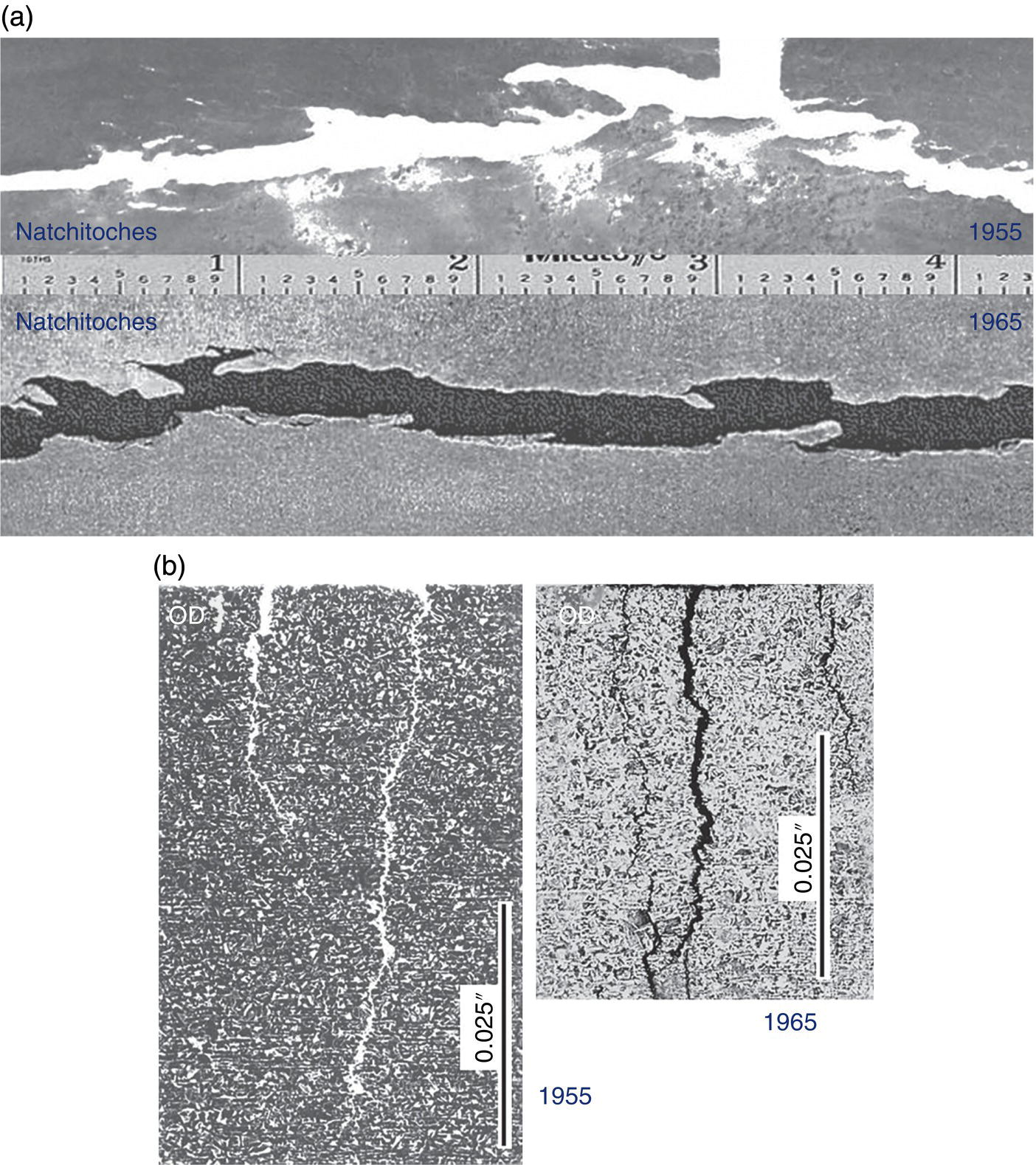
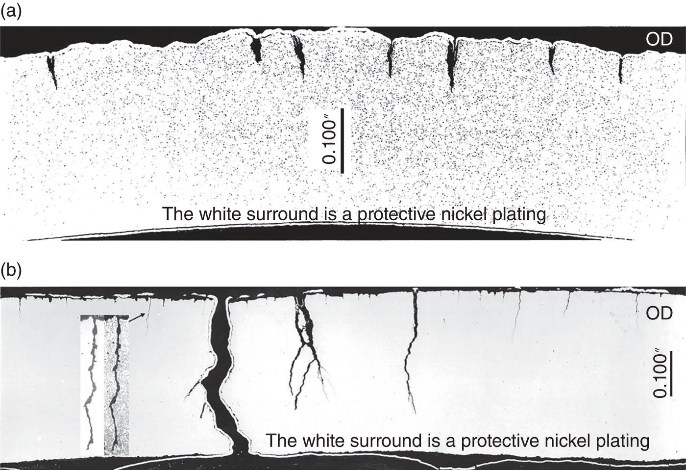
53.2 Research Concerning the Factors Controlling SCC2
53.2.1 Early Years through Present-Day: The Roles of Temperature and Potential
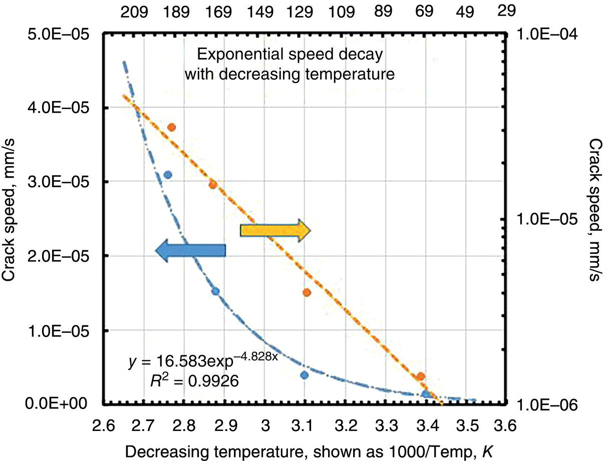
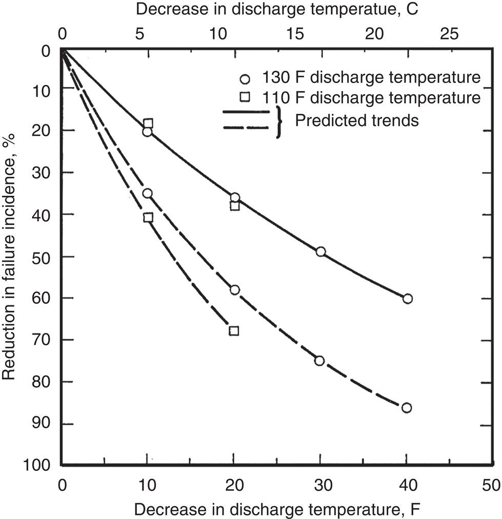
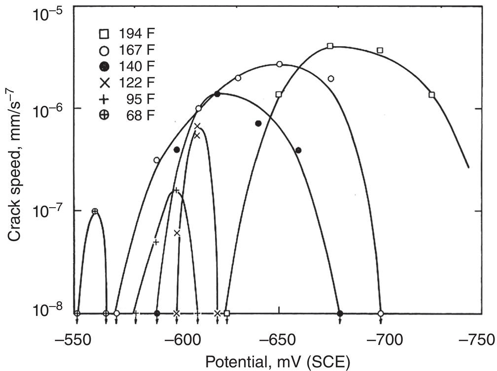
53.2.1.1 Effect of Temperature on SCC Susceptibility and Initiation Cracking Speed
53.2.1.2 Field-Calibrated Effect of Temperature on SCC Incidence
53.2.1.3 Effects of Potential on SCC Susceptibility and Cracking Speed
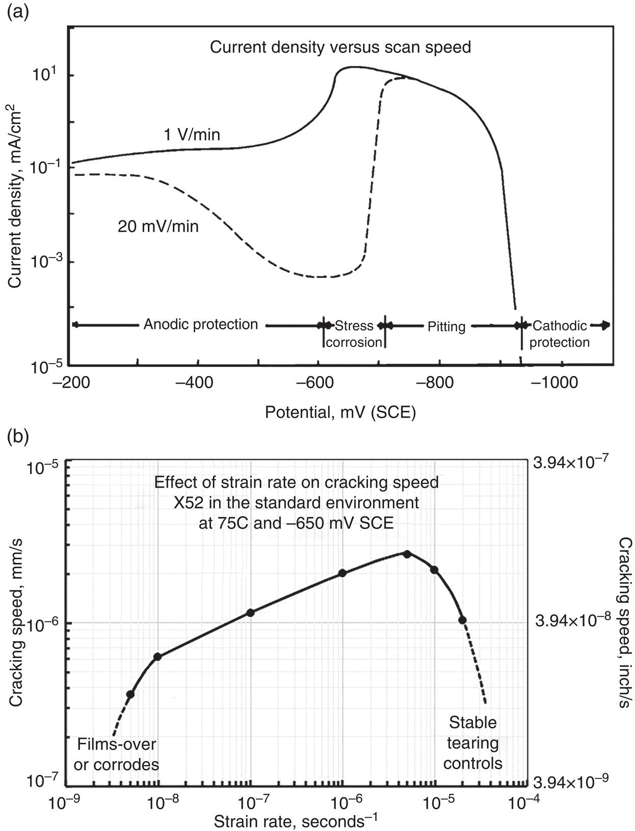
53.2.2 Active–Passive Cracking from Smooth Surfaces: The “Free-Surface Effect”
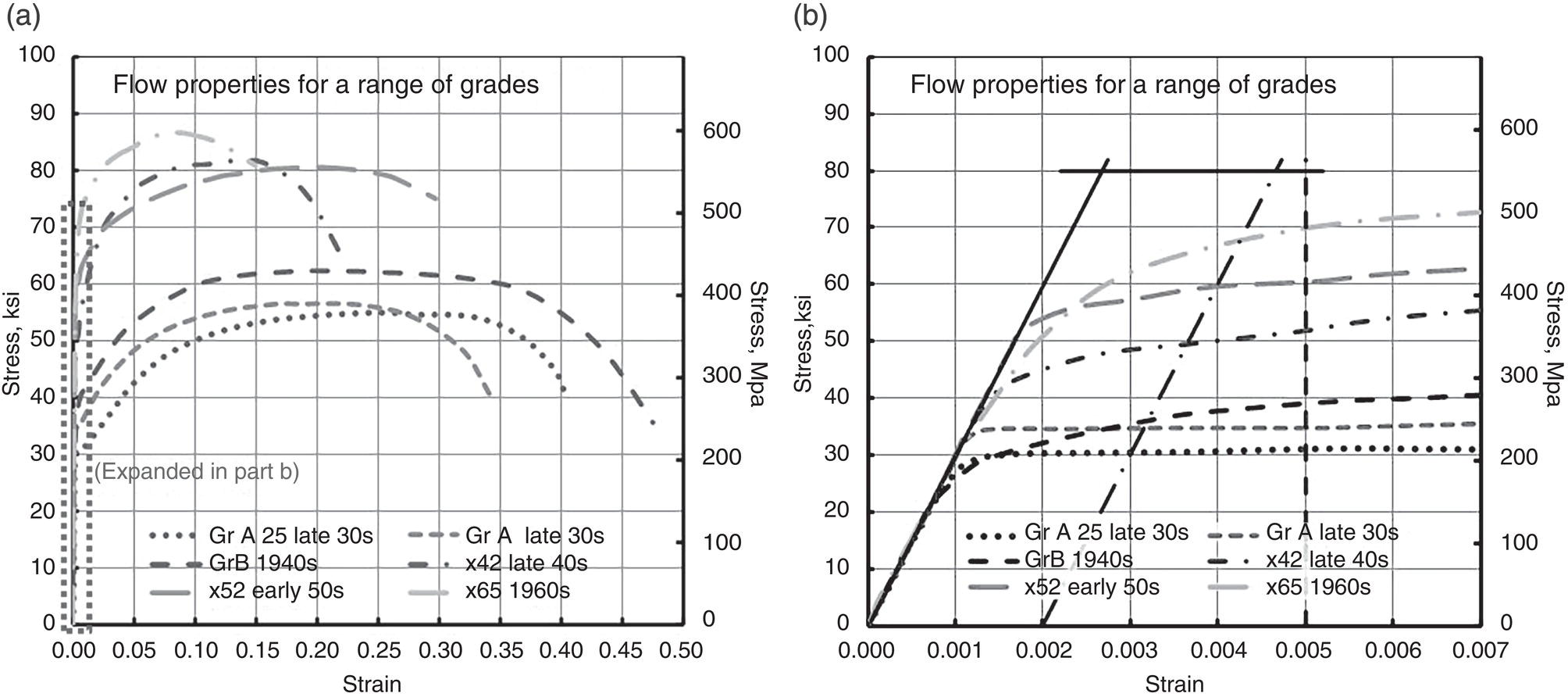
53.2.3 Effect of Stress: Thresholds and Cracking Speeds for High-pH SCC
53.2.3.1 Crack Initiation Threshold and Related Cracking Speeds

53.2.3.2 SCC Speeds for Growth from Crack-Free Surfaces: Smooth Specimens
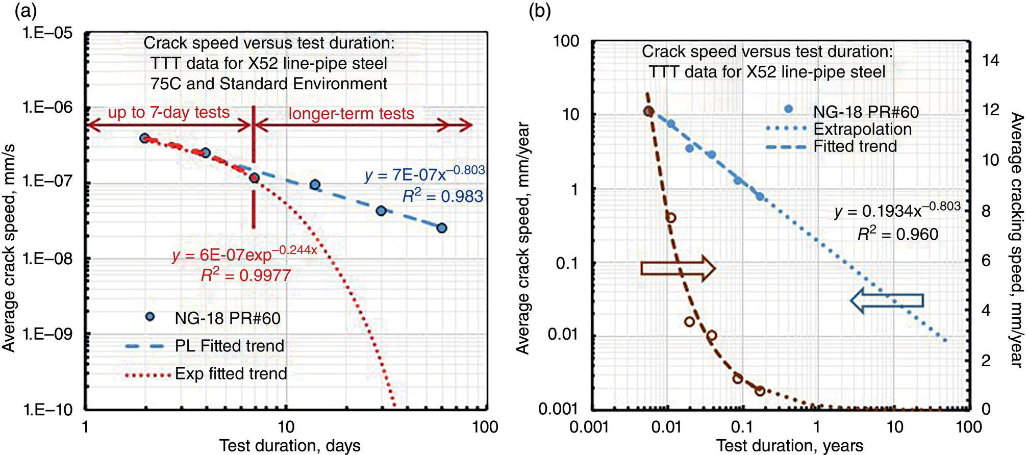

53.2.3.3 Macrocrack Propagation Threshold and Crack Speed: Temperature Effects
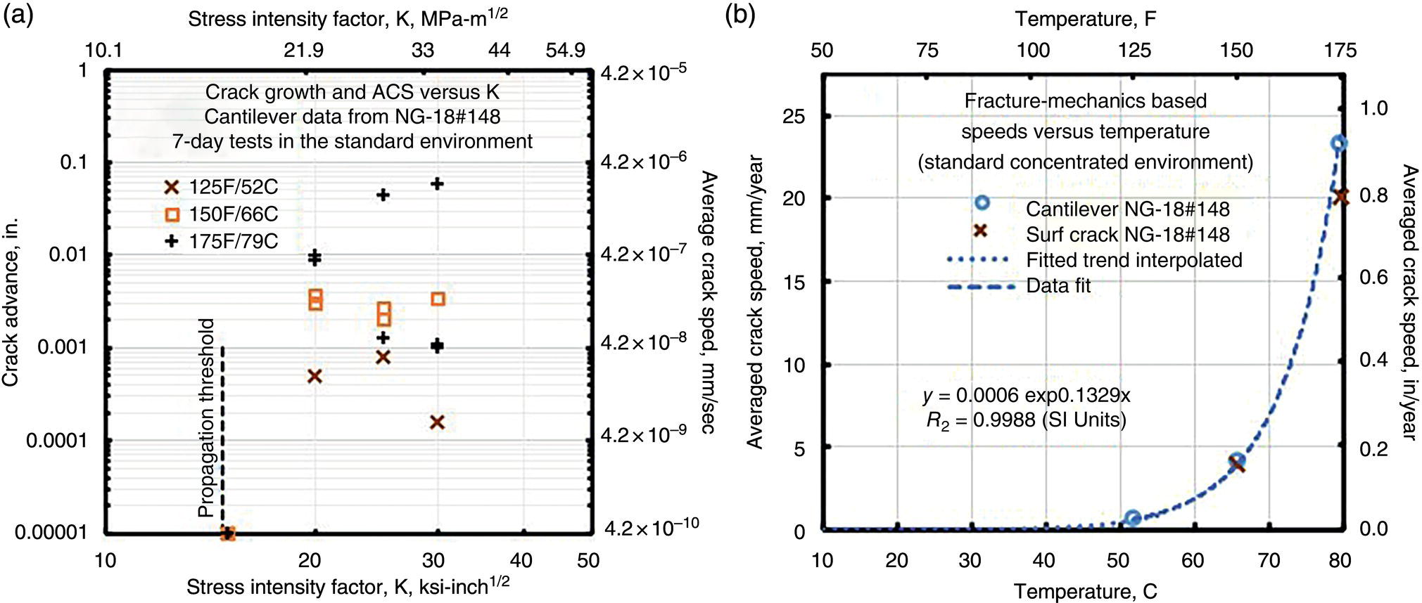
53.2.4 Transition from Initiation and Early Growth to Macrocrack Propagation
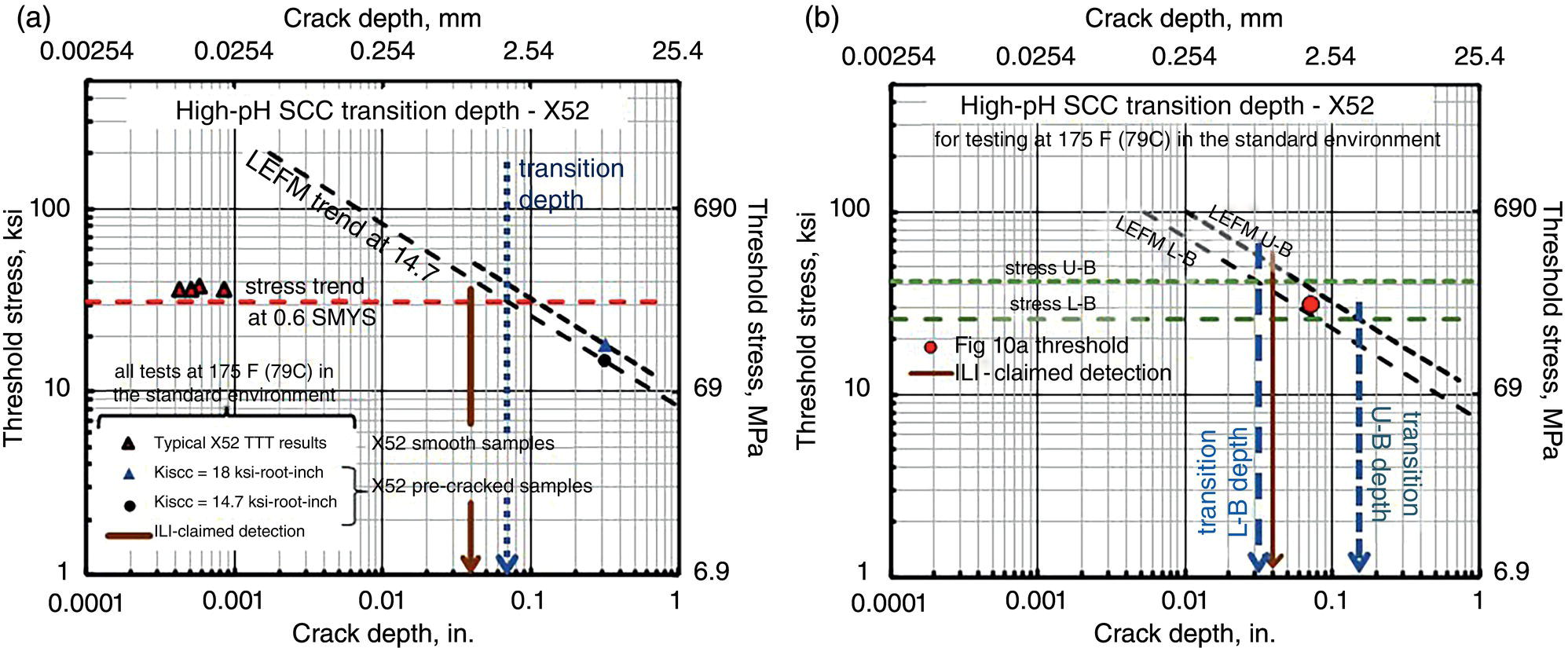
53.3 Factors Controlling SCC—Service Versus Laboratory Cracking
53.4 Quantifying a Bathtub Speed-Life Curve for High-pH SCC
53.4.1 The Bathtub Curve and its Adaptation to SCC
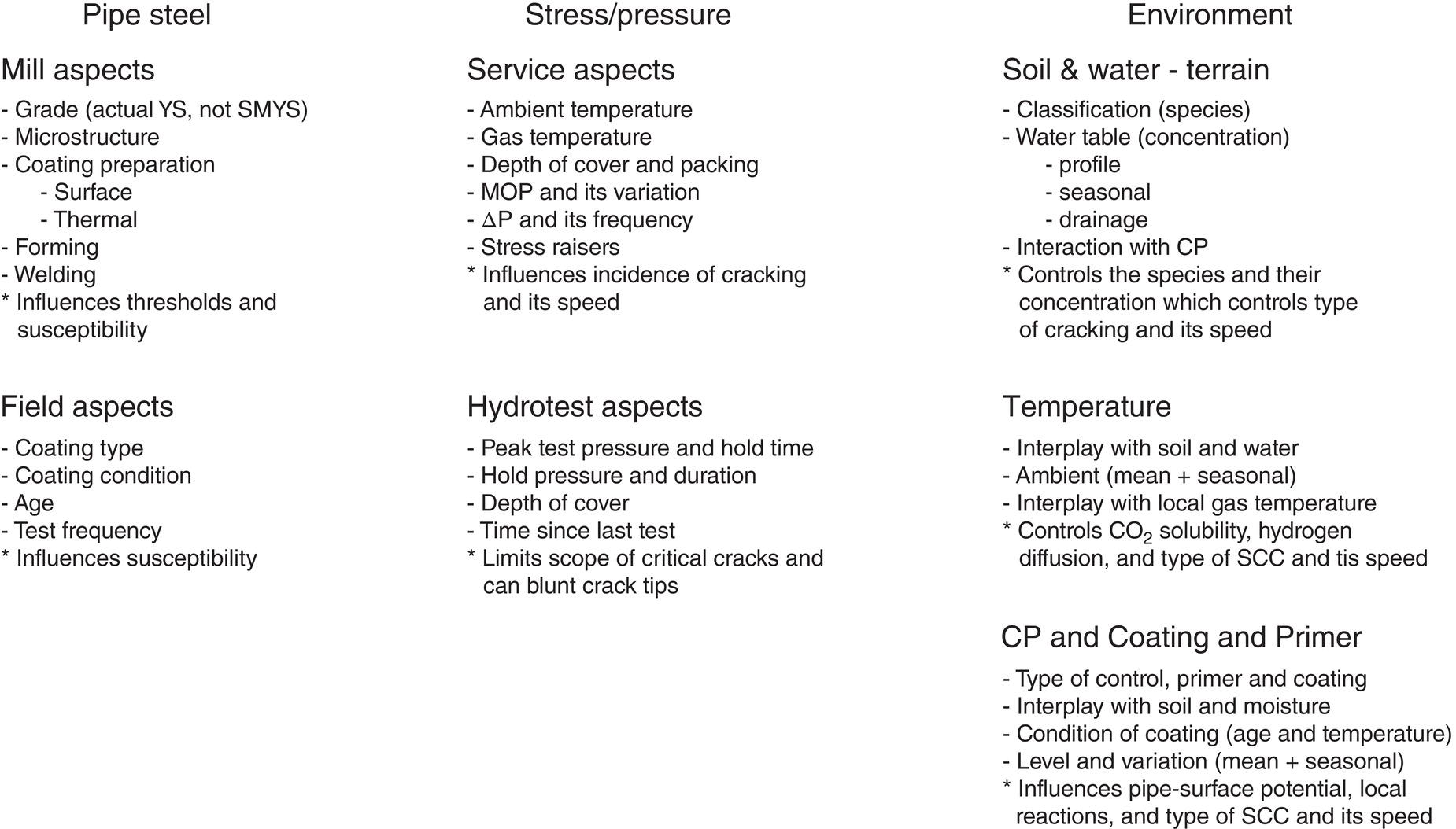
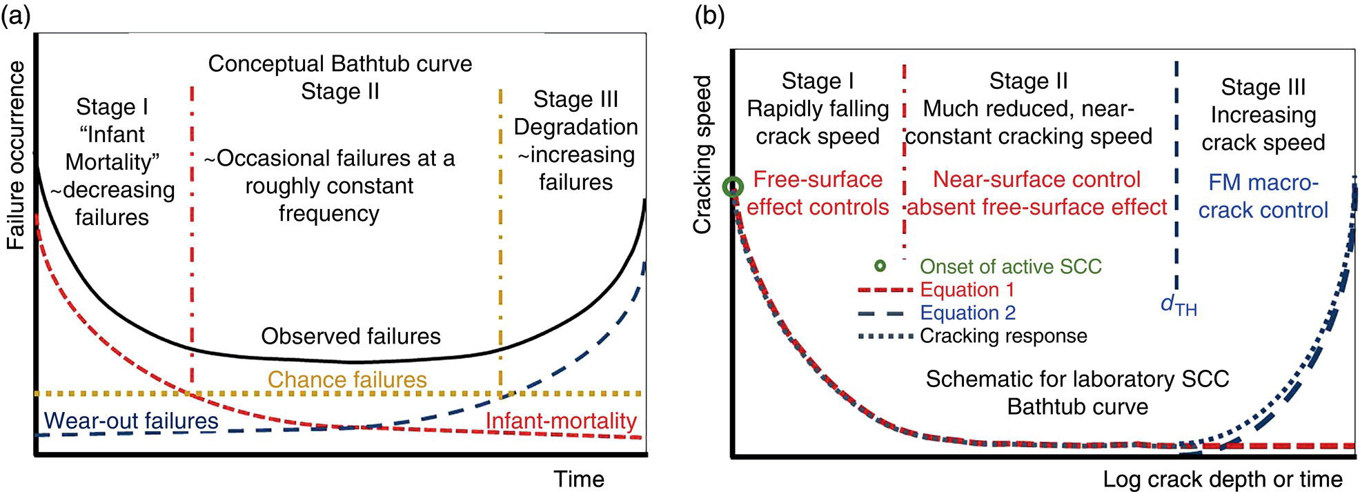
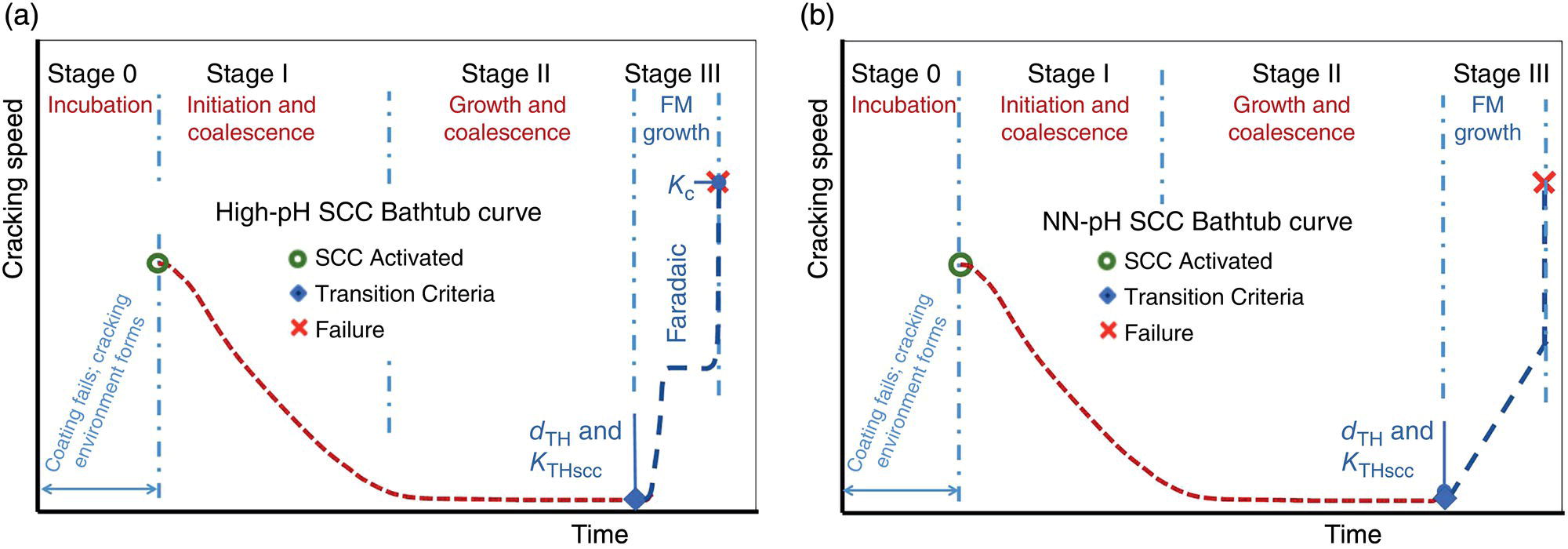
53.4.2 Simulated Bathtub Life Curves for Susceptible and Resistant Pipe Steels
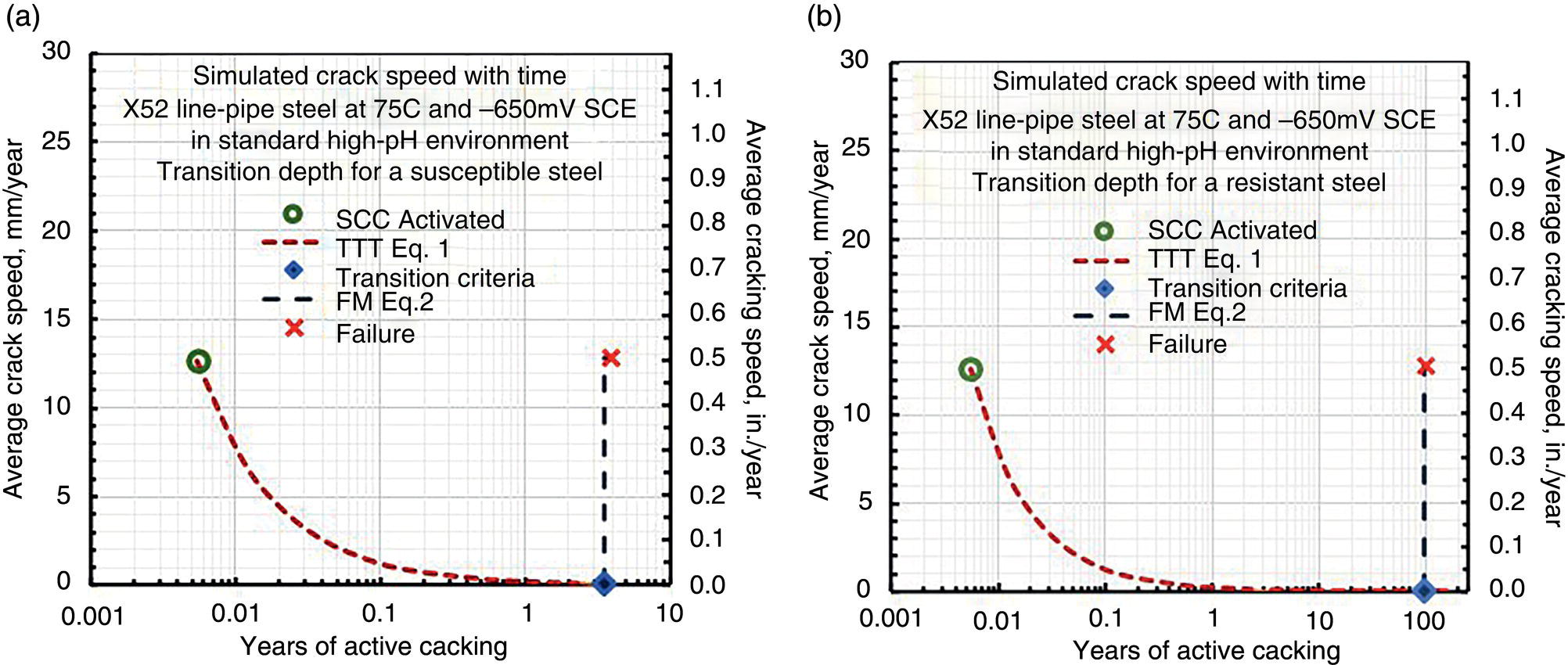
53.4.3 Incubation
53.4.4 Broadening the ACS Database for Field Cracking
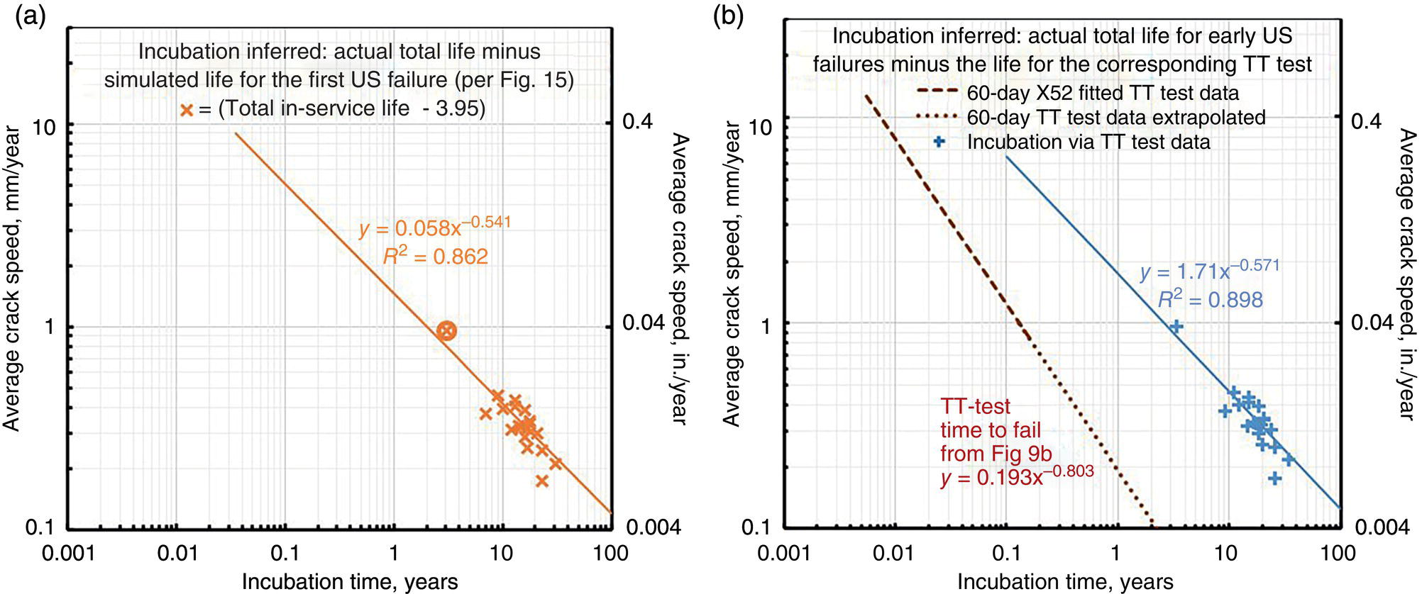

53.4.5 Observations and Practical Takeaways
53.5 Emergence of NN-pH SCC: Its Traits Versus High-pH SCC
Parametera
High-pH
Near-Neutral pHb
Other names
Classical
Low-pH, non-classical
Systems
Higher stress-ratioc pressure pipelines in gas and hazardous liquid transmission service
Location
Often <30 km downstream (D/S) from a pump or compressor station, but not always as it has been found much further D/S
D/S from compressor/pump station—initially worse in the first valve section, it is migrating system wide (depending on pressure range and cyclic frequency)
Reversed/reversing flows require SCC management review/oversight
As the environment is reversible, both forms of SCC can be found on the same pipeline; in some cases, in the same mainline valve section
Nominal operating conditions
Historically occurred at MOP ≥ 60% of SMYS; more recent experience indicates failures at much lower stresses; most have occurred above 60%
Age
Earliest in < 7 years, the majority > 20 years
Several in < 15 years, the majority > 20 years
Coating and conditiond
Commonly associated with disbonds under coal tar, followed by tapes
Most common under disbonds in tapes, asphalt, and wax coatings
Electrolyte, pHe, and reaction products
Concentrated aqueous carbonate–bicarbonate solution with 8.4 < pH < 11
Carbonate-bicarbonate side of CO2H2O system with black deposits of magnetite and often siderite
Dilute aqueous bicarbonate–carbonic acid solution with 4.5 < pH < 8.4
Carbonic acid–bicarbonate side of CO2H2O system with FeCO3 as a reaction product (useful discriminator) and black deposits of magnetite and often siderite
Temperature
Crack speed decreases exponentially with decreasing temperature—failure frequency decreases with decreasing temperature
No strong correlation with temperature, but the solubility of CO2 increases as temperature decreases, which has implications for cracking
Electrochemical aspectsf
Off-potential used to determine CP level
Susceptible within a very narrow range of potentials
CP ranges in the field from −0.70 to −1.4 V
At free corrosion potential (−0.6–−0.9 V) for asphalt—but not a factor for tape coatings
Can be shielded—depends on coating
Shielded conditions or inadequate CP
Note that coatings other than tape affect shielding
Terrain (soil type, drainage, topography)
Can occur in dry/well-drained soils where CP can be ineffective—also can be found in damp to wet transitions in clay/silt textured soils
Varies: occurs in bogs, on through dry soils
Depends on at least the type of coating and its condition
Conditions that decrease coating adhesion and increase shielding accelerate coating degradation
Cracking locationsg
Generally in the pipe body, under disbonded coatings, occasionally also found near/in seams—and other stress raisers
Areas of locally higher stress and disbonded coating like girth and long-seam welds (toe cracking), also in the pipe body often in external corrosion/pitting
Crack morphologyh
Primarily IG, but in banded steels can be TG or mixed, often with limited pipe surface and crack-flank corrosion; in x-section it typically appears tight, and shows fine branched cracking
Primarily TG, sometimes mixed with IG at crack tips; pipe surface pitting and crack-flank corrosion are common; x-sections often show wide corroded cracks, often with compacted corrosion debris, and limited branching
53.6 Industry Guidance on Crack Speed and the Incidence of SCC
53.6.1 Cracking Speed
53.6.2 Where and When SCC Might be Anticipated
53.7 Interface between Integrity and Condition Assessment
53.7.1 Background
53.7.1.1 Oil and Gas Industry Developments Circa 2000
53.7.1.2 Regulatory Developments and Mandates Pending Circa 2000
53.7.2 Detection and Sizing SCC15
53.7.2.1 Definitions
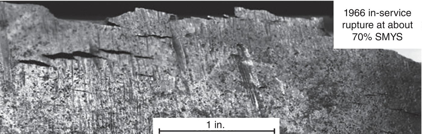
53.7.2.2 ILI Output Versus the IM Analyst’s Hopes and/or Expectations
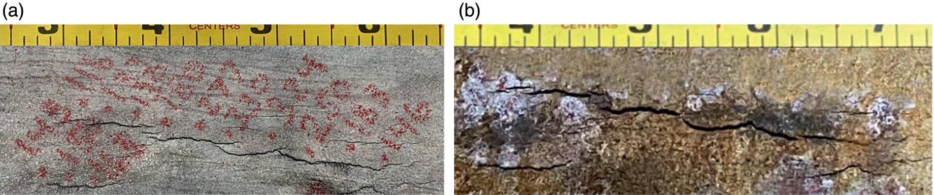
53.7.2.3 Crack Aspect Ratio and Its Implications
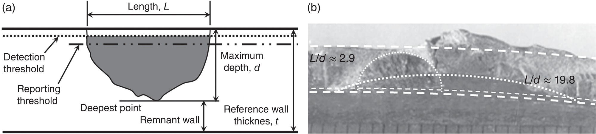
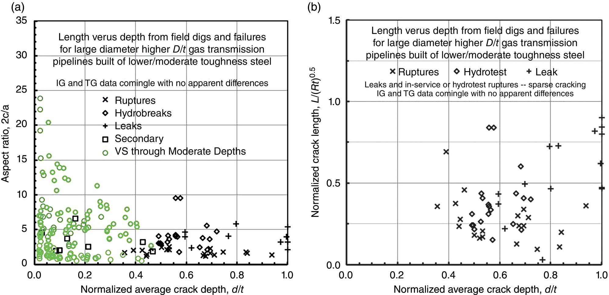
53.7.3 Reporting Thresholds—Analysis, Implications, and Takeaways
53.7.3.1 Analyses and Outcomes
Depth, d
% of t
Shaded for Depth ≤ a Reporting Threshold of 1 mm (0.0394 in.)
Wall thickness, t, inch or mm in adjacent columns
0.250 or 6.35
0.312 or 7.92
0.360 or 9.14
0.400 or 10.2
0.500 or 12.7
10%
0.025
0.635
0.031
0.792
0.036
0.914
0.040
1.016
0.050
1.270
15%
0.038
0.953
0.047
1.189
0.054
1.372
0.060
1.524
0.075
1.905
20%
0.050
1.270
0.062
1.585
0.072
1.829
0.080
2.032
0.100
2.540
25%
0.063
1.588
0.078
1.981
0.090
2.286
0.100
2.540
0.125
3.175
30%
0.075
1.905
0.094
2.377
0.108
2.743
0.120
3.048
0.150
3.810
40%
0.100
2.540
0.125
3.170
0.144
3.658
0.160
4.064
0.200
5.080
50%
0.125
3.175
0.156
3.962
0.180
4.572
0.200
5.080
0.250
6.350
60%
0.150
3.810
0.187
4.755
0.216
5.486
0.240
6.096
0.300
7.620
70%
0.175
4.445
0.218
5.547
0.252
6.401
0.280
7.112
0.350
8.890
80%
0.200
5.080
0.250
6.340
0.288
7.315
0.320
8.128
0.400
10.160 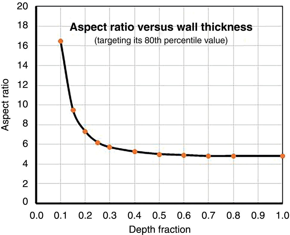
Approx Bounds on L/d
L/d at ~80th Percentile
Depth, d, % of t
Shaded for Length ≤ a reporting threshold of 1 in. (25.4 mm)
Corresponding Length, L, as a Function of Wall Thickness, inch or mm
0.250 or 6.35
0.312 or 7.92
0.360 or 9.14
0.400 or 10.2
0.500 or 12.7
0.5–24
16.5
10%
0.413
10.48
0.515
13.1
0.594
15.1
0.660
16.8
0.825
21.0
1.8–17.7
9.5
15%
0.356
9.05
0.445
11.3
0.513
13.0
0.570
14.5
0.713
18.1
2–7.9
7.3
20%
0.365
9.27
0.456
11.6
0.526
13.4
0.584
14.8
0.730
18.5
2 to 8.5
6.2
25%
0.388
9.84
0.484
12.3
0.558
14.2
0.620
15.7
0.775
19.7
2–8.1
5.7
30%
0.428
10.86
0.534
13.6
0.616
15.6
0.684
17.4
0.855
21.7
2–7.1
5.3
40%
0.525
13.34
0.655
16.6
0.756
19.2
0.840
21.3
1.05
26.7
2–5.6
5.0
50%
0.625
15.88
0.780
19.8
0.900
22.9
1.000
25.4
1.25
31.8
2–4.9
4.9
60%
0.735
18.67
0.917
23.3
1.058
26.9
1.176
29.9
1.470
37.3
2–5.1
4.8
70%
0.840
21.34
1.048
26.6
1.210
30.7
1.344
34.1
1.680
42.7
2–5.8
4.8
80%
0.960
24.38
1.198
30.4
1.382
35.1
1.536
39.0
1.920
48.8
53.7.3.2 Representative Unity Plot—Observations and Implications
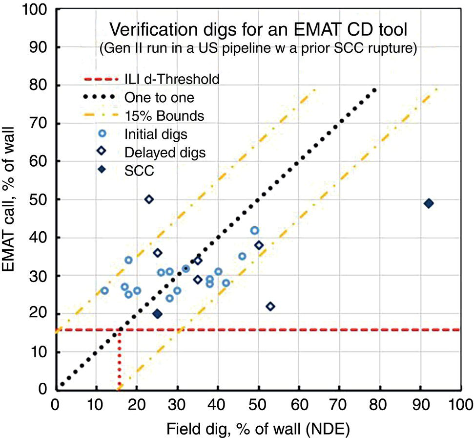
53.7.3.3 Takeaways
53.8 Summary and Conclusions
Acknowledgments
References21,22,23,24,25,26
Notes
Factors Controlling Stress Corrosion Cracking and Typical Growth Rates


(53.1b)
