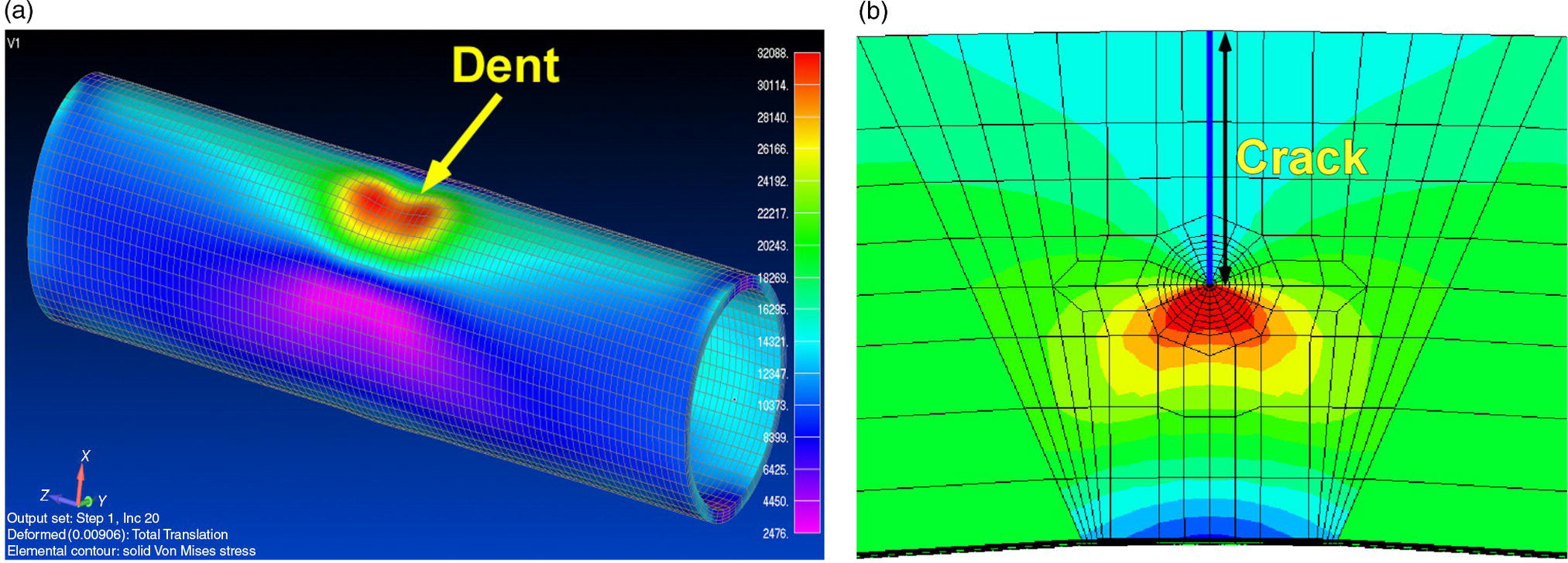
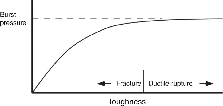
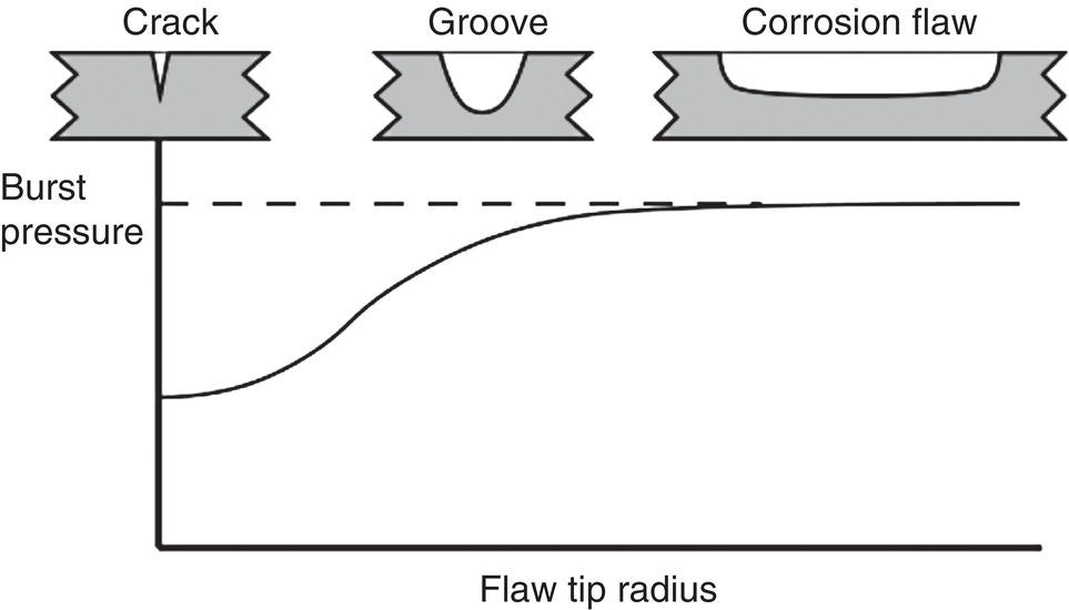
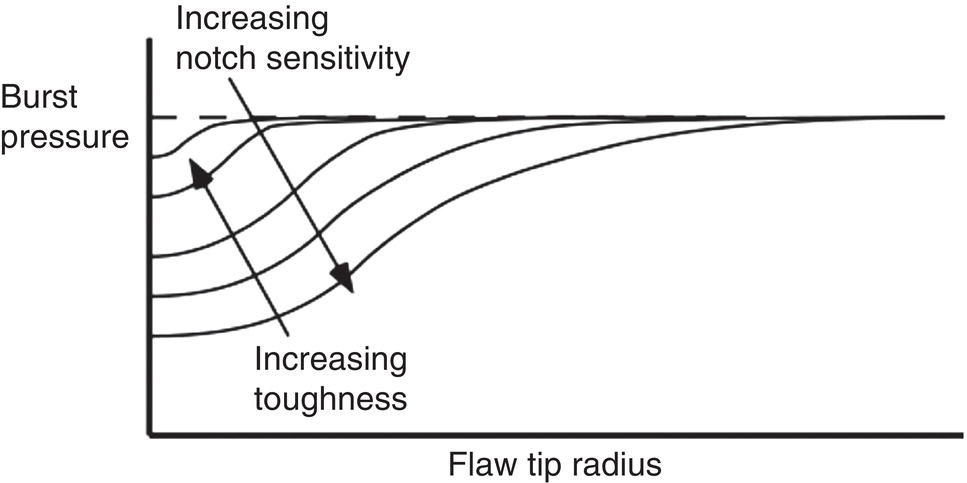
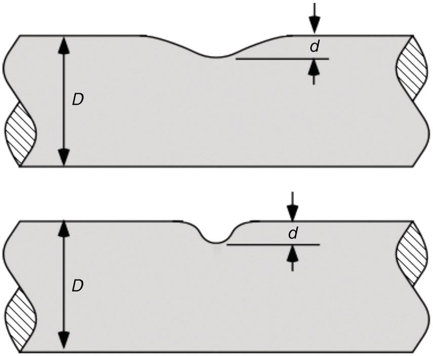
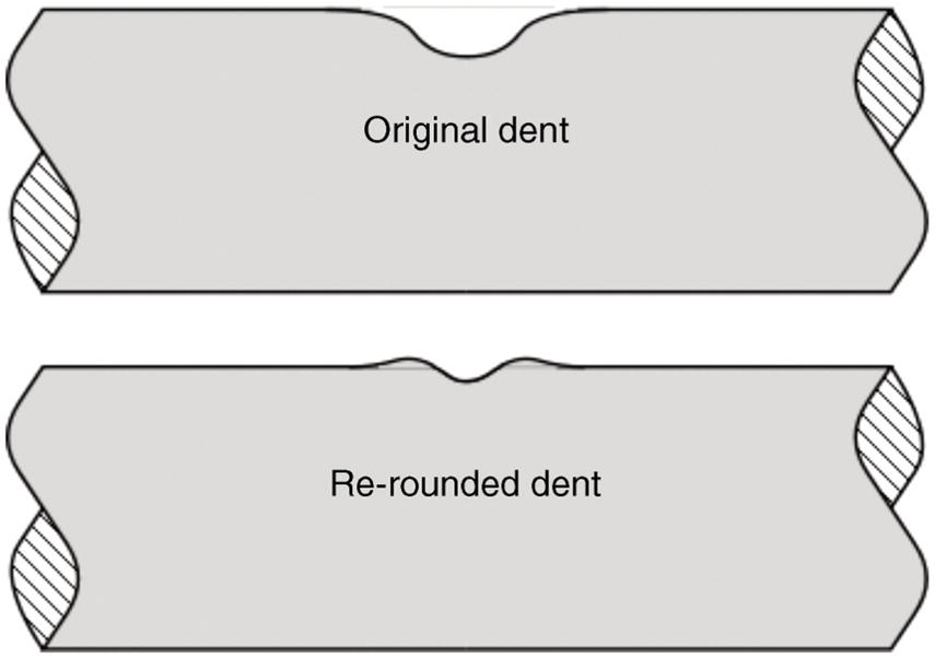
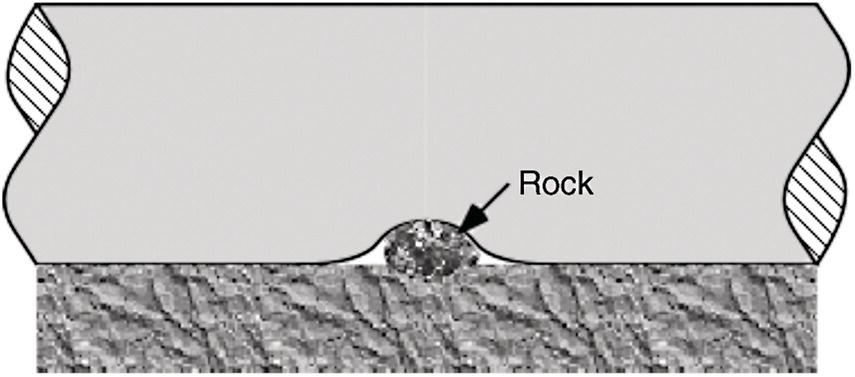
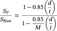
Ted L. Anderson TL Anderson Consulting, Cape Coral, FL, USA Flaws in a pipeline can reduce the burst pressure and shorten the life of the line. The vast majority of releases that have occurred in pipelines can be attributed to flaws. Some flaws are introduced at the time of manufacture, while others develop in service. Table 35.1 lists the most common flaw types. Various flaw assessment procedures are available to predict the effect of flaws on burst pressure and remaining life. Such procedures are a crucial part of an effective integrity management program. For example, remaining life calculations are typically used to establish appropriate intervals for hydrostatic testing and in-line inspection (ILI). A fundamental reason why flaws can adversely affect pipeline integrity is that these imperfections act as stress concentrators. Figure 35.1 shows two finite-element models that illustrate this effect. Figure 35.1a is a color stress map of a dented pipe under pressure loading. The deviation of a pipe from a cylindrical shell results in much higher stresses in the dent compared with the rest of the pipe. Figure 35.1b is a color stress map at the tip of a crack, which is the most severe type of stress concentrator. Part of the reason for the stress concentration is local reduction in wall thickness, but the sharpness of the flaw magnifies this effect significantly. A notch-like feature, such as a lack-of-fusion flaw, has a lower stress concentration factor (SCF) than a crack, and a smooth metal loss flaw has a lower stress concentration than either a crack or a notch. In the case of crack-like flaws and metal loss, the high local stress at the flaw reduces the burst pressure. Burst tests on dented pipes usually do not show a significant reduction in burst pressure, but dented pipes can fail over time by fatigue, which is driven by cyclic pressure. Metal loss and crack-like flaws can grow over time, which gradually reduces burst pressure until it reaches the local operating pressure. The response of pipelines to flaws is influenced by material properties. The following properties affect the burst pressure: When the pipe reaches its burst pressure, the failure mode may either be ductile rupture or fracture. In the former case, the burst pressure is governed by the tensile properties, while fracture is controlled by toughness. In a fracture event, the pipe essentially unzips, as a crack rapidly propagates. Toughness is defined as the ability of the material to resist rapid crack propagation. Traditionally, the toughness of pipeline steels and welds has been quantified by Charpy tests, but toughness tests based on fracture mechanics principles have seen increasing use in the pipeline industry in recent years. Figure 35.2 schematically illustrates the effect of toughness on burst pressure of a pipe that contains a longitudinal crack-like flaw. In the fracture regime, burst pressure increases with toughness. At high toughness levels, a plateau is reached where the failure mode changes to ductile rupture, which is controlled by tensile properties. In other words, increases in toughness eventually produce diminishing returns at high toughness levels. For time-dependent damage mechanisms, such as fatigue, corrosion, and stress corrosion cracking (SCC), material properties in addition to those listed previously may influence the damage rate. Initiation of fatigue is influenced by strength, but fatigue crack growth rates are insensitive to tensile properties. Environmental degradation mechanisms such as corrosion and SCC are driven by complex interactions between the environment and the material. Table 35.1 Common Flaw Types At low–moderate toughness levels, the sharpness of a flaw can have a significant effect on burst pressure. Figure 35.3 illustrates the typical trend. Sharp cracks result in the lowest burst pressure because of the stress concentration effect described earlier. As the notch radius increases, the failure mode transitions from fracture to ductile rupture. Failure at smooth metal loss flaws generally occurs by ductile rupture, where tensile properties govern the strength of the pipe. Figure 35.1 Finite element models with color stress maps that show stress concentrations due to pipeline flaws. (a) Stress concentration at a dent. (b) Stress concentration at the tip of a crack. Figure 35.4 illustrates the combined effect of toughness and notch acuity. Low toughness materials are notch-sensitive, in that the burst pressure is sensitive to the notch tip radius. By contrast, the burst pressure for high toughness materials is insensitive to notch acuity (sharpness). In this case, a pipe with a longitudinal crack of a given length and depth will have essentially the same burst pressure as a pipe (made from the same material) with a metal loss flaw with the same length and depth. A number of procedures are available for assessing metal loss in pipelines, including B31G [1], API 579 [2], as well as a DNV Recommended Practice [3]. These methods differ somewhat in minor details, but they all are based on research performed at Battelle Laboratories in the late 1960s and early 1970s [4]. The modified B31G procedure, described in this section, is widely used to assess flaws in pipelines. Figure 35.2 Effect of toughness on burst pressure in a pipe that contains a longitudinal crack. Figure 35.3 Effect of notch acuity (sharpness) on burst pressure in a pipe that contains a longitudinal flaw. Figure 35.4 Combined effect of toughness and notch acuity on burst pressure. Figure 35.5 Sketch of a metal loss flaw, where L is the length in the longitudinal direction and d is the depth. Consider a metal loss flaw with longitudinal extent L and maximum depth d, as illustrated in Figure 35.5. According to the modified B31G method (level 1), the remaining strength of a corroded pipe is given by where SF is the hoop stress at failure in the corroded pipe and Sflow is the flow stress. The parameter M is called the Folias factor or the bulging factor and is given by where z is a dimensionless function of flaw length, L; wall thickness, t; and pipe external diameter, D: The underlying assumption of Equation 35.1 is that a pipe without corrosion will fail when the hoop stress reaches Sflow. The B31G method gives several alternative definitions of flow stress, including 1.1 SMYS, SMYS + 69 MPa (10 ksi), and the average of SMYS and SMTS. All of these definitions are conservative, as an unflawed pipe will typically burst when the hoop stress is approximately equal to the tensile strength. API 579 refers to the ratio on the left-hand side of Equation 35.1 as the remaining strength factor (RSF). The RSF is the ratio of the strength of the corroded pipe to that of the uncorroded pipe. The reciprocal of the RSF can be viewed as an SCF. In other words, the nominal hoop stress and the local hoop stress in the remaining ligament of the flaw are related through the RSF (=1/SCF): Equation 35.1 predicts the burst pressure that must be divided by a safety factor to obtain the maximum allowable operating pressure (MAOP) for the corroded pipe. B31G recommends a safety factor of 1.39 for pipelines with an allowable hoop stress of 72% SMYS. Since 1.39 = 1/0.72, this implies that the corroded pipe can have a local hoop stress, When wall thickness has been mapped with multiple readings, usually on a grid, a more advanced method called effective area can be used to assess metal loss. Both B31G and API 579 include the effective area method as level 2 assessment. Given a thickness map over the area of interest, a “river-bottom” profile is taken, which corresponds to the longitudinal path of minimum thickness through the flaw. The thickness readings along the river bottom profile are then projected onto a 2D plane. The resulting thickness profile is subdivided into sections and subjected to a series of RSF calculations using a modified version of Equation 35.1. Note that in the level 1 procedure already discussed, only the length, L, and maximum depth, d, are used in the calculation, while the effective area method accounts for the shape of the thickness profile. Figure 35.6 depicts two corrosion flaws with the same L and d, but with different thickness profiles. The level 1 method would predict the same burst pressure for the two flaws, but the effective area method would account for the additional reinforcement in flaw A and thus predict a higher burst pressure for this case. Figure 35.6 Comparison of two metal loss flaws with the same length and maximum depth. The B31G level 1 method (Equation 35.1) predicts that both flaws will have the same burst pressure, but the level 2 effective area method accounts for the actual flaw profile. Cracks can pose a greater threat to pipeline integrity than metal loss flaws. A sharp crack is a much more severe stress concentrator than a metal loss flaw of the same length and depth. Cracks and other planar flaws result in a significant decrease in burst pressure for materials that are notch-sensitive (Figure 35.4). Moreover, cracks can grow in service by fatigue or through environmentally assisted corrosion mechanisms such as SCC. Fracture mechanics is a relatively new engineering discipline, which predicts the effect of cracks on structural integrity [5]. There are three key variables in a fracture assessment, as illustrated in Figure 35.7. A typical fracture mechanics model consists of an equation that relates stress, flaw size, and toughness. Given one equation and three unknowns, it is necessary to specify two quantities in order to calculate the third. For example, if stress and toughness are known, it is possible to calculate the critical crack size for fracture. Note that the variables in Figure 35.7 are grouped into two categories: driving force and material resistance. The driving force, which is a function of stress and crack size, promotes crack propagation, while the toughness is a measure of the ability of the material to resist crack propagation. Fracture occurs when the driving force exceeds the material resistance. Fracture is more likely with either stress or crack size increase since both quantities affect the driving force. As an analogy, consider plastic deformation (yielding) in metals. In this case, the applied stress can be viewed as the driving force for yielding, while the yield strength is a measure of the material resistance to yielding. Figure 35.7 The three key variables in a fracture mechanics analysis. The stress and crack size influence the driving force for fracture (i.e., the forces that are trying to propagate the crack) while the toughness is a measure of the material resistance to fracture. A suitable fracture mechanics model can be used to compute the burst pressure in a pipe, given the crack dimensions and material toughness. Figure 35.8 is sketch of a crack stability diagram for longitudinal cracks in a pipeline. For a fixed material toughness, burst pressure is plotted against crack length for part-through surface cracks of various depths. The diagram also shows the burst pressure versus crack length curve for a through-wall crack. Note that the predicted failure pressure for short, deep cracks is less than the failure pressure for through-wall cracks of the same length. The physical meaning of this result is that the remaining ligament of the short, deep crack can fail, but the resulting through-wall crack is stable, in which case a leak occurs rather than rupture of the pipe. If the failure pressure for a part-through crack is above that of the corresponding through-wall crack, the analysis predicts that the pipe will rupture when the critical pressure is reached. During the Battelle research that resulted in a model for volumetric metal loss flaws, the authors [4] observed that the metal loss equation overpredicted the burst pressure of pipes with sharp notches, especially for pipes with low Charpy toughness. They concluded that a burst pressure equation for crack-like flaws needed to account for material toughness. At the time of the Battelle project (circa 1970), the field of fracture mechanics was in its infancy, and the fundamental understanding of failure of structures containing cracks was limited. A rigorous model for axial cracks in pipelines was simply beyond the state of knowledge at the time. The Battelle research team developed a semi-empirical burst pressure equation for longitudinal cracks that was based on a simplistic model that was published in 1966 [6]. The original model, as well as the Battelle equation, contained a secant function as the argument of a natural logarithm. Consequently, the Battelle equation became known as the log-secant model. This model predicts the burst pressure versus toughness trend depicted in Figure 35.2, and it reduces to the B31G metal loss equation when toughness is large. The log-secant model has been used extensively by the pipeline industry since it was first published. Over time, weaknesses in the model became apparent. For example, the model is excessively conservative for long, shallow flaws. In fact, this model predicts that a superficial longitudinal scratch on the pipe (d/t → 0) will result in a large drop in burst pressure relative to a pristine pipe. In 2008, Kiefner [7] published a modified version of the log-secant model that was intended to address shortcomings in the original equation. While the modification helped mitigate the problem with long, shallow cracks, it introduced another problem. Namely, the modified log-secant equation predicts that burst pressure is insensitive to toughness, which is an obviously incorrect result. Figure 35.9 is a plot that compares the burst pressure predictions for the original and modified log-secant equations. The field of fracture mechanics has advanced considerably since 1970, and better models are available to predict the relationship between burst pressure, crack size, and toughness in pipelines. The modified log-secant model does not incorporate recent advances in fracture mechanics. Rather, it merely applies a multiplying factor to the original equation. For reasons described ahead, the failure assessment diagram (FAD) approach is vastly superior to both the original and modified log-secant models for assessing crack-like flaws in pipelines. Figure 35.8 Crack stability diagram that is a plot of burst pressure versus flaw dimensions. The failure assessment diagram (FAD) method is based on sound fracture mechanics principles. This methodology appears in a number of Standards, including API 579 [2] and the British Standard BS 7910 [8]. A recent study [9] demonstrated that the API 579 FAD method was significantly better at predicting burst test results than the original and modified log-secant methods. In addition to being based on modern fracture mechanics principles, the FAD method is more versatile than the log-secant methods. The FAD method applies to both longitudinal flaws and circumferential flaws, but the log-secant methods pertain only to longitudinal flaws. Also, the FAD method accounts for the differences between cracks on the OD versus ID of the pipe, and it incorporates weld residual stresses when appropriate. The log-secant methods do not distinguish between ID and OD cracks, nor do these methods account for weld residual stress. Figure 35.10 schematically illustrates the FAD. Given a particular pressure and crack size, the pipe is assessed by calculating the toughness ratio (the y coordinate) and the load ratio (the v coordinate) and then plotting the point on the FAD. In simplified terms, the toughness ratio is a check on brittle fracture,1 while the load ratio is a check on yielding and ductile rupture. The FAD curve interpolates between the extremes of fully brittle and fully ductile failure. If the assessment point falls inside of the curve, the crack is predicted to be stable. Failure is predicted if the point falls outside of the curve. Figure 35.9 Comparison of burst pressure predictions from the original and modified log-secant models. Figure 35.10 The FAD. If the assessment point falls within the FAD curve, the flaw is stable. Failure is predicted when the assessment point falls outside of the FAD curve. Figure 35.11 Calculation of burst pressure with the FAD method. Given an arbitrary pressure, p, the ratio of burst pressure to p is equal to the ratio of the line segments OB and OA. The assessment point is computed for a given pressure and crack size. An iterative procedure is required to compute the critical crack size. First, the assessment point is computed for an initial guess of the critical crack size. If the point falls inside the FAD curve, the crack size is gradually increased until the point falls on the curve. If the initial guess falls outside of the FAD curve, the crack size is decreased until the assessment point falls on the curve. Figure 35.11 illustrates the procedure for determining burst pressure with the FAD method. Given an arbitrary pressure p that results in an assessment point A, the burst pressure is inferred from the distance from the origin to A relative to the distance from the origin to B, which lies on the FAD curve: A variation of this procedure is used when weld residual stresses are included in the analysis. Preexisting flaws in a pipeline can grow by fatigue when the pressure oscillates frequently. Fatigue crack growth is predominantly a problem in liquid lines but can also occur in gas lines. In addition to predicting the critical conditions for burst in a pipe that contains a crack-like flaw, fracture mechanics concepts can be used to predict the rate at which a crack grows due to cyclic pressure. Figure 35.12 illustrates the steps involved in pressure cycle fatigue analysis. First, the pressure versus time data are processed through an algorithm called rainflow counting [10]. This results in a histogram of cyclic pressure (Δp) versus number of binned cycles at each Δp. The cyclic pressure histogram is then input into a fracture mechanics-based fatigue crack growth model. An initial crack size must also be input into this model, along with relevant material properties. The initial flaw size can be based on ILI data, or it can be inferred from a hydrostatic test. That is, if a section of a pipeline passes a hydrotest, then it is possible to infer the size of the largest cracks that could have survived the test. The fatigue crack growth analysis predicts how long it will take for the flaw to grow from the initial size to a critical size at which point failure is predicted. The calculated remaining life is typically used to set the interval for the next ILI run or hydrostatic test. In most cases, this interval is set to half the estimated remaining life. Dents are the most common source of failure in pipelines, but they are the least understood flaw type. Although there are established models and methods to assess metal loss and cracks, dents are usually handled with rule-based approaches. Existing regulations for dents are based primarily on experience and general rules of thumb. Figure 35.12 The steps involved in a pressure cycle fatigue analysis. Pressure versus time data are processed through a rainflow cycle counting algorithm, resulting in a cyclic pressure histogram. The histogram is then input into a fatigue crack growth analysis. Leaks and ruptures at dents are usually caused by fatigue.2 The dent results in a stress concentration that magnifies cyclic stresses. A 3D finite element analysis of the dented pipe, such as shown in Figure 35.1a, is usually required to estimate remaining life. Simple formulas based on dent dimensions are insufficient for estimating accurate stresses for life assessment. The primary dent characterizing parameter in rule-based dent acceptance criteria is the ratio of the dent depth to the pipe diameter. This parameter does not tell the complete story of a dent, however. The sketches in Figure 35.13 depict two dents of the same depth/diameter ratio. In one case, the dent is smooth and gradual, while the dent is sharper and more abrupt in the other case. The latter dent has a greater SCF than the former and will have a shorter fatigue life. The constraint on the pipe can also affect fatigue life, along with the size and shape of the dent. Figures 35.14 and 35.15 illustrate unconstrained and constrained dents, respectively. An unconstrained dent tends to re-round with pressure cycling, as illustrated in Figure 35.14. Consequently, by the time a dent is detected by ILI, it may look considerably different than when it first formed. In the case of a constrained dent, such as a rock dent at the 6 o’clock position (Figure 35.15), the dent typically retains its original shape. Although an unconstrained dent that has re-rounded often looks less severe than a constrained rock dent, the latter may actually have a longer fatigue life. The constraint on the dent that prevents it from re-rounding with pressure cycling also reduces the stresses in the dent. Figure 35.13 Sketches of two dents with the same depth/ diameter ratio but with different shapes. The sharper and more abrupt dent will have a shorter fatigue life than the smooth and gradual dent. Dent constraint tends to vary with position around a buried pipe. A dent at the 12 o’clock position usually experiences less constraint from the overburden relative to a dent at 6 o’clock that is resisted by a solid foundation. Figure 35.14 Illustration of an unconstrained dent. The shape and depth of the dent change over time as the dent re-rounds with pressure cycling. Figure 35.15 Illustration of a dent that is constrained by a rock at the bottom of the trench in which the pipe was buried.
35
Flaw Assessment
35.1 Overview
35.1.1 Why Are Flaws Detrimental?
35.1.2 Material Properties for Flaw Assessment
Flaw Classification
Examples
Metal loss
Localized corrosion and pitting
General wall thinning
Gouges
Cracks and crack-like flaws
Hook cracks in ERW seams
Lack-of-fusion flaws
Fatigue cracks
Stress corrosion cracks
Dents
Constrained or unconstrained dents
Sharp or smooth dents
Dents with metal loss
Dents at welds
35.1.3 Effect of Notch Acuity
35.2 Assessing Metal Loss

 , equal to 0.72 Sflow rather than 0.72 SMYS. Note that if the corrosion flaw is small or shallow, the B31G acceptance criterion can result in an allowable pressure that is greater than the original design pressure, in which case the pressure reverts to the original MAOP.
35.3 Crack Assessment

35.3.1 The Log-Secant Model for Longitudinal Cracks

35.3.2 The Failure Assessment Diagram

35.3.3 Pressure Cycle Fatigue Analysis
35.4 Dents
References
Notes
Flaw Assessment
(35.2)
(35.3)
(35.4)
(35.5)