section epub:type=”chapter” role=”doc-chapter”> Accelerated corrosion in gas turbine engines, boilers, and other high temperature systems is usually caused by the existence of combustion products in a liquid phase. In the chemical industry, the molten salts used as a heat transfer medium are compatible with construction materials, and corrosion is an inevitably serious problem. Thus far, there have been many reports from both theoretical and experimental viewpoints and fundamental approaches made by Simons et al. (1955), Goebel and Pettit (1970), Mamantov (1969), and others, who suggested with sufficient credibility the electrochemical mechanistic models for the observed corrosion. In fact, most of the molten salts behave as ionic or electrolytic conductors, and therefore it is easy to understand that the molten salt corrosion at high temperature is of electrochemical nature, as it happens in aqueous systems. Accordingly, high temperature electrochemistry is of great importance in understanding and controlling molten salt corrosion. But the scientists and engineers concerned with high temperature corrosion problems need also to deal with metals, alloys, ceramics, composites, and other advanced materials of difficult processing. Moreover, the diversity of interests in advanced technology applications at high temperature oblige them to be concerned with complex environments, namely, gaseous atmospheres containing oxygen, hydrogen, carbon dioxide, water vapor, sulfides, chlorides, etc. At high temperatures, these gaseous atmospheres lead to the growth of thin oxide layers, compact scales, and multilayered scales. Most of these layers and scales are ionic compounds or, at least, partially ionic compounds. Thus, the chemical reactions established at solid–solid and solid–gas interfaces during the growth of the corrosion products can be visualized as oxidation–reduction electrode processes; in other words, it is acceptable that high temperature oxidation, sulfidation, halogenation, nitridation, carburization, etc. are processes of electrochemical nature. In summary, it is clear that the extension of electrochemistry to high temperature materials and systems (Garcia‐Diaz et al. 2016) that are highly susceptible to corrosion will constitute an important tool that requires further exploration (Wildgoose et al. 2004). In this chapter, basic aspects of molten salt electrochemistry and solid‐state electrochemistry are described to show how molten salt corrosion and high temperature oxidation can be further understood and mitigated. The loss of material is substantially attributed to the corrosion reaction, and therefore the material surface suffers from the homogeneous or heterogeneous attack of corrosive media. For the former case, Wagner and Traud (1938) described the fact that the occurrence of the corrosion reaction necessitates simultaneous dissolution of metals and reduction of oxidant. According to their theory, the location of the metal dissolution is not necessarily identified with that of oxidant reduction at the metal–solution interface. Therefore, the important factors in corrosion are not only impurities, defects, and other heterogeneities of the material but also the chemical nature of the oxidant involved in the liquid (i.e. impurities and by‐products due to dissociation). From this viewpoint, the corrosion reaction in molten salts is a fairly complex phenomenon compared with that in an aqueous medium where only a few chemicals such as oxygen and protons might be candidates for the oxidant of the corrosion reaction. It should be noted that while in aqueous solutions metals are virtually insoluble in the electronated state, in molten or fused salts (which can be regarded as infinitely concentrated aqueous solutions), they can be appreciably soluble and corrosion occurring, in such cases, without the de‐electronation of the metal. In spite of this, the electrochemical approach for molten salt systems was put forward about 55 years ago and is finding general acceptance. Based on the mixed potential theory, the corrosion reaction is expressed by the combination of metal dissolution, partial anodic reaction and reduction of oxidant, and partial cathodic reaction under the restriction of electric charge neutrality: thus, for the partial anodic reaction, and for the partial cathodic reaction, where M, Ox, and R represent the metal, oxidant, and reductant, respectively, and n is the number of electrons. Accordingly, in a molten salt, there are several oxidants (O2, H+, H2O, and OH−) common to the molten salts, and such oxidants are associated with the dissociation reaction of molten salts themselves. At this stage and before moving further to thermodynamic considerations, it is important to briefly describe the meaning of the electrode potential, which is the central electrochemical parameter. In the most general sense of the word, an electrode is a system consisting of two phases in contact with each other, which can be the seat of an electrode reaction, i.e. a reaction in which certain constituents of the two phases participate and by which a transfer of charge takes place from the bulk of one phase to the bulk of the other. In a more restricted sense, an electrode is defined as a metal–electrolyte or metal–solution system of one or several electrolytes. It has been shown over the last 100 years that at the interface of two phases, one finds an electrical double layer with a characteristic potential (Adam 1938; Butler 1940). The origin and the characterization of the electrochemical double layer on a metal immersed in an aqueous electrolyte have been extensively studied. Similar studies in melts have been carried out only more recently. This section is not intended to deal with this aspect in detail, but the subject is mentioned because of its importance. Very good reviews on the subject have been published by Devanathan and Tilak (1965), Graves et al. (1966), and Ukshe et al. (1964). Returning to the subject of this section, let the inner electric potential of the metal be ΦM and that at a remote point in the molten electrolyte be ΦS. Moreover, let ΔΦ represent the Galvani electric potential across the electrochemical double layer, i.e. ΔΦ = ΦM − ΦS. When a dynamic equilibrium across the double layer is set up, the electrochemical energy of 1 mol of metal in the surface will be equal to the electrochemical free energy of 1 mol of ions on the melt side of the double layer: or and where μM − μS is the chemical energy balanced by the electrical energy liberated as Mn+ ions traverse the double layer, F is Faraday’s constant, and n is the number of free electrons exchanged at the Mn+/M interface. It is impossible to measure ΔΦ directly, but if the metal–melt electrode system is coupled “back to back” with a second arbitrarily chosen electrode system, it is possible to obtain a relative potential difference. If a zero potential and a convenient reference scale of potentials is defined, the combined system acts as a cell between those electrodes and there exists an electromotive force (e.m.f.) given by where E0.4 is called the single potential of the Mn+/M electrode on the chosen standard reference scale. Considering now a more concise electrode reaction, where Mi represents the constituents of the electrode taking part in the reaction and e− represents the electron; the corresponding conditions of dynamic equilibrium can be expressed in the general form Relating the chemical potentials, μi, to the standard chemical potential, Table 6.1 Basicities pO2− of various molten salts where pgas is the partial pressure of the gas Changing from natural to Briggsian logarithms, the last relation can be rewritten in the form in which Equation 6.10 is the Nernst equation. Thermodynamic considerations can predict whether a metal is stable or whether it will corrode when it coexists with the oxidants common to molten salts. When the metal dissolution in Eq. 6.1 and the oxidant reduction in Eq. 6.3 are taken into account, the free energy of the global reaction associated with them can be negative, i.e. the potential difference ΔE(= E0.3 − E0.1) is positive, and therefore corrosion proceeds spontaneously. Since the metal reacts with chemical species such as oxide ions and oxyanions that constitute the molten salts, the equilibrium potential varies with the activity of the oxide ion in the melts. Hence, the diagram of chemical entities in the melt as a function of the electrode potential and the basicity is helpful in a comprehensive understanding of the corrosion behavior. The basicity of the melt is defined as pO2− ( where KT indicates the equilibrium constant of Eq. 6.12. Table 6.1 shows typical acid–base equilibria and the pO2− equation for these molten salts. The equilibrium diagrams E–pO2− and its construction are fully described in Section 3.3.1 for the iron/sodium sulfate system at 1173 K. Similar diagrams for molten salts including single, binary, and ternary salt mixtures are also published in the open literature (Ingram and Janz 1965; Kunst and Duke 1963; Littlewood 1962; Marchiano and Arvia 1972; Rahmel 1968; Sequeira and Hocking 1977). Thermodynamically calculated E–pO2− diagrams have resulted in remarkable progress in understanding corrosion, but this method has several (qualitative) disadvantages for the realistic requirements of design engineers. In particular, the domains of thermodynamic stability considered in the diagrams give only a theoretical possibility of existence, not a certainty. Further on, as far as passivation is concerned, it must be pointed out that a proper passivity in molten media has not been obtained up to date, perhaps due to special properties of the film involved, mainly adherence, coherence, and deviation from stoichiometry. Therefore, elaborate kinetic techniques for obtaining precise corrosion rates are needed. Figure 6.1 Polarization curves of a fast electrochemical reaction. (a) Arithmetic scale for i. (b) Logarithmic scale for i. Figure 6.2 Polarization curves of a slow electrochemical reaction. (a) Arithmetic scale for i. (b) Logarithmic scale for i. Considering now the dynamic side of the corrosion phenomenon, particular importance will be attached to electrochemical kinetic studies. A classic relationship precisely relating a characteristic parameter of the electrode, its electrode potential, and the current density traversing it is that found by Tafel in 1905. Therefore this semiempirical law enables us to establish a connection between the “thermodynamic electrode potential” and the current density that defines the kinetic character of the phenomenon. The Tafel equation may be written as where E is the relative electric potential of the electrode at a current density i (also called “reaction‐electrode potential”), a is a constant characteristic of the electrode, and b is the Tafel slope, which is one of the parameters indicating the mechanism of the electrode reaction. Thus, a definition of overpotential for the reaction can be introduced by the expression where E0 is the reversible or equilibrium electric potential possessed by the electrode at electrochemical equilibrium (i.e. at zero imposed current) or, more generally, the equilibrium potential of the electrochemical reaction of the type (Eq. 6.7). Equation 6.15 defines the overpotential, and considering Eq. 6.14, it is seen that the Tafel equation is itself closely related to the overpotential (η). These problems of electrochemical kinetics are discussed in more detail later. The brief discussion given above is significant enough for the present purpose of showing that the Tafel relationship leads to the experimental polarization curves. Figures 6.1 and 6.2 represent the anodic and cathodic potential–current curves for two typical electrochemical reactions, with either an arithmetic scale for the reaction current (Figures 6.1a and 6.2a) or with a logarithmic one (Figures 6.1b and 6.2b). The exchange current density (i0), which is defined as the exchange rate per unit area of the potential‐determining electrode process at equilibrium, is represented in Figures 6.1b and 6.2b. The aspect of the polarization curves is very important because it gives an account of the degree of irreversibility of the reactions. In fact, in the case of a reversible reaction (Figure 6.1), the application of very small polarizing potentials is sufficient for producing significant current densities. In the case of irreversibility (Figure 6.2), on the contrary, the existence of high overpotentials is a measure of the extent of irreversibility. The reversible or fast electrode processes exhibit high exchange current densities; on the other hand, the irreversible or slow ones exhibit low exchange current densities. Thus, if an electrode is more likely to behave reversibly, the higher is its intrinsic exchange current density. The Tafel curves giving E as the function of log i also provide interesting results about the kinetics of the phenomena. In fact, the plot of E against log i is not usually a straight line, i.e. the kinetics of the reaction does not obey the Tafel relation. The experimental curves obtained can be considered as built up of rectilinear portions or, on the contrary, as showing systematic departures from the linear Tafel relation for certain current densities reached. It is well established in electrochemistry that the Tafel relation does not apply precisely for small and large current densities. One reason for this is that the Tafel equation is derived purely by considering the overpotential due to polarization caused by charge transfer requirements, which assumes that a cation moves away from the metal‐fused electrolyte interface as soon as it is dissolved. This is generally not the case. The removal of the anodic product does not increase in the same proportion as the current density and the concentration of these products will increase and cause a back e.m.f. This effect is particularly relevant in the case of fast electrode processes as observation of Figures 6.1 and 6.2 shows: the difficulty in obtaining a pure Tafel slope, i.e. unaffected by double layer and mass transfer effects, increases with kinetics of the electrode processes (i.e. with high i0) due to increasing overlapping of the diffusion zones over the Tafel one. Polarization measurements also include ohmic overpotential that arises from an IR drop through a portion of the electrolyte and between the test electrode and the reference one, but this term is not significant in molten media as compared with an aqueous system. The validity of the Tafel equation has been verified by Laitinen and Gaur (1957), Randles and White (1955), and others for many fused systems. The facts mentioned above are very important especially due to their repercussion on the interpretation of electrochemical phenomena. So, it is seen, by this simple enumeration, that it is possible to connect thermodynamic considerations to kinetic ones. In the section above, where some concepts of electrode kinetics were discussed, a quantity of crucial importance to electrodics was defined: the overpotential (η). In electrochemical kinetics, the only reaction directly affected by the potential is the charge transfer reaction, i.e. the reaction in which charge carriers are transferred across the electrochemical double layer at a phase boundary. The rate of the charge transfer reaction determines the charge transfer or activation overpotential. This kind of overpotential has been treated in detail by Audubert (1942), Bard and Faulkner (1998), Bockris (1954), Butler (1924), Conway (1965), Erdey‐Gruz and Volmer (1930), Gerischer (1960, 1961), and others. Figure 6.3 Corrosion of a metal M in a molten sulfate with SO2 evolution. Anodic and cathodic polarization curves. Corrosion potential and corrosion current. (a) Representation with an arithmetic scale for the reaction current. (b) Representation with a logarithmic scale for the reaction current. Prior to discussion, it is noted that only the basic electrodic equations will be considered. Considering the conversion of M+ ions into metallic M, the number of moles of positive ions reacting per second by crossing unit area of the melt–metal interface is proportional to the electronation current density i and as a first approximation (Erdey‐Gruz and Volmer 1930): where and also a de‐electronation reaction In this case, the total current density passing through the double layer is where {M} is the activity of the metallic atoms immediately at the electrode surface (unity). If the metal–melt interface reaches its equilibrium state, there is no net current (i = 0), but there is an exchange current. The electronation and de‐electronation reactions continue to occur but at the same rate. The current densities corresponding to these individual reactions become the exchange current density i0 (i0 = i+ = |i−|). Hence, where E0 is the potential difference across the interface at equilibrium. On dividing Eq. 6.19 by the corresponding expressions in Eq. 6.20 and taking into consideration the definition for overpotential η, the following important relationship is obtained (Erdey‐Gruz and Volmer 1930): For higher charge transfer overpotentials, |η| > RT/F, the first or second term on the right‐hand side (r.h.s.) of Eq. 6.21 can be neglected depending on the sign of the current so that if this Eq. 6.21 is put into a logarithmic form, a linear relationship results between η and log|i| similar to the Tafel equation: Here, the subscripts “+” and “−” to the overpotential denote anodic and cathodic polarization, respectively. Let us now consider the following reaction of a metal M in a molten sulfate (Burrows and Hills 1966): This overall reaction can be considered as the sum of the two half‐reactions: For these two processes to take place simultaneously, it is necessary and sufficient that the potential difference across the interface be more positive than the equilibrium potential for the reaction 6.24 and more negative than the equilibrium potential of the electronation reaction 6.25 involving electron acceptors (such as SO3) contained in the melt: The behavior for the potential–current curve E(I) that can be envisaged for the process Eq. 6.23 is illustrated in Figure 6.3 by the continuous thick line. (I) E is composed additively of the metal dissolution current I24 (E) and the electronation current I25 (E), and the two are independent of each other at the same potential value. The principle of additive combination of all partial processes at an electrode surface to obtain the total potential–current curve was first formulated by Wagner and Traud (1938). The potential E at zero current is neither E0.25 nor E0.24, but a so‐called mixed potential (EM) for which the total potential–current curve gives I (EM) = 0. The total metal dissolution current I24 and electronation current I25 are then equal in magnitude but opposite in sign, i.e. The rate of corrosion of the metal is obviously given directly by the rate of metal dissolution; hence, the free corrosion current Ic (i.e. the rate at which the metal destroys itself) is given by Considering the electrode kinetics, we can thus write where A24 is the sink area and A25 is the electron‐source area (at the metal–electrolyte interface). Assuming that overpotentials are sufficiently large, Eqs. 6.30 and 6.31 become The free corrosion potential, Ec, i.e. the uniform potential difference over the surface of the corroding metal, can be evaluated from the expressions above. It follows that It is clear from this that the free corrosion potential and the mixed potential are identical. In accordance with the theory of Lux (1939) and Flood et al. (1952) who assign a definite acid–base equilibrium to all oxyanionic melts, the acid–base equilibria for sulfates can be expressed by the Eq. 6.12 and by the equilibrium constant Assuming where pO2− = − log {O2−} is a nonprotonic function that measures the acidity of the melt, as already reported. The expression 6.35 for the active species SO3 can be introduced into Eq. 6.33, giving Assuming that the ratio of A25 and A24 as well as α24 and α25 is constant during the overall corrosion reaction (which is not free from error), Eq. 6.36 becomes with a and b being two constants. Thus, we attain a linear relationship between the corrosion potential and the function pO2−, which should be valid for all oxyanionic melts. What has been presented above is a very elementary account of electrodics of corrosion under quite ideal conditions. The details of the complex corrosion phenomena in real systems are out of the scope of this chapter. In this section, an account is given of several available methods for obtaining the potential–current curves, the free corrosion rates, and the electrochemical monitoring of corrosion. It is customary to classify the electrochemical methods for obtaining such potential–current curves into potential‐sweep, current‐sweep, potential‐step, and current‐step methods. The former method, sometimes called potentiodynamic (or potentiokinetic) polarization, is accomplished by continuously changing the applied electrode potential (with feedback control) at a constant rate and simultaneously recording current. In the current‐sweep (intensiokinetic) method, the electrolysis current (with feedback control) is varied with time according to a given program, and the electrode potential is recorded as a function of current. In the potential‐step method, electrode potential is rapidly changed over a finite increment, and current measured after a predetermined time interval, and this process is repeated. In the last (above) method, a current step is applied, and the resulting variation of potential with time is recorded. These two‐step methods are also referred to as potentiostatic and galvanostatic (or intensiostatic), respectively, to indicate that at any instant E (or I) is held constant, by means of feedback control. All the polarization methods described above are well established in the ambient temperature range (Edeleanu 1958; Greene 1962; Greene and Leonard 1964; Pourbaix and Vandervelden 1965; Prazak 1963) for electrochemical studies of metals, the best or most accurate of them depending, of course, on its intended use: if the purpose is to study the kinetics phenomena, the methods in which the electrode potential is controlled are the best; when the permanent physicochemical modifications, due to applied current, are the objective, the methods in which the electrolysis current is controlled are preferable. Generally speaking, however, potential‐step and potential‐sweep methods will be more useful for the study of corrosion phenomena than current‐step and current‐sweep methods because they give more precise indications concerning the quality of the passivation and concerning the conditions of activation. The investigation of corrosion processes in melts by these standard electrochemical techniques was pioneered by a reasonable number of researchers (Arvia et al. 1971, 1972a, b; Baudo et al. 1970; Davis and Kinnibrugh 1970; Kazantsev et al. 1968; Sequeira and Hocking 1978a, b, 1981), and, in general, it can be said that almost all workers in the field of high temperature agree that the polarization methods appear to be quite suitable in corrosion studies at high temperature in molten electrolytes. The polarization curves have several shapes, but near the potential axis their character is similar to that shown by the curves plotted in Figures 6.1 and 6.2. A potentiodynamic polarization curve provides a graphic summary of the corrosion characteristics of tested material so that its plot and evolution can be used as a very rapid and practically nondestructive corrosion test. However, the corrosion characteristics obtained are accurate only for the medium in which the curve was obtained. Therefore, the importance of the method does not lie in any final evaluation of the rates of corrosion in a particular medium, but rather in the rapid evaluation of fundamental corrosion properties with the possibility of sensitive relative comparison (Prazak 1963). Another feature of the method is that analysis of such potential–current curves, together with E − pO2− diagrams, enables us to predetermine those reactions theoretically possible and impossible for each electrode potential value. One of the most important electrochemical values for the determination of the kinetics and mechanisms of primary corrosion processes is the value of the free corrosion current. When the primary corrosion process is slow (absence of concentration polarization), the free corrosion current can be obtained by potentiodynamically polarizing the alloy electrode at a very slow sweep rate in the neighborhood of the free corrosion potential. The alloy dissolution rate is obtained by plotting potential versus log current, and extrapolating the linear anodic and cathodic branches is the free corrosion potential, the intercept giving the free corrosion current. This method can also be applied when some (relatively small) concentration polarization is present; the latter can be taken into account by using the approximate expression where Imeas. is the measured current in the presence of concentration polarization and Id is the diffusion current (of course this correction implies the exact knowledge of the diffusion current). When the primary corrosion processes are sufficiently fast, other methods, namely, relaxation methods, must be used. The objective of these methods is the study of the electrode processes before they become diffusion controlled. The experimental techniques associated with these methods are very complex, but they are the most important ways allowing accurate determination of fast charge transfer corrosion rates. Several relaxation methods for these measurements have been considerably revised by Graves and Inman (1970), and useful exposition of the “classical” relaxation methods is that of Damaskin (1967). The selection of the method to measure the free corrosion currents, depending precisely on rate phenomena, is obviously difficult (because the values of these corrosion rates are not known a priori). In general, the high temperatures of fused salt systems cause most corrosion processes to be rapid (reversible with respect to the non‐relaxation methods). Generally speaking, therefore, relaxation methods will be the most appropriate for the determination of corrosion rates in melts. The measurement of free corrosion rates in molten salts was pioneered by Baudo et al. (1970) and Cutler (1971), among others. The first workers determined the corrosion rates using the conventional method, extensively and successfully applied at low temperatures in aqueous systems; they presented the results in the form of Tafel plots, but they do not give information on the current–potential measured values from which the plots of E versus log i were obtained. It is rather surprising in view of the relatively high corrosion rates quoted that it had been possible to obtain pure Tafel zones. It is certain that this method enables the measurement of rough values (more of qualitative than quantitative value) of the free corrosion rates, but it is advisable to put into practice LaQue’s opinion that new and more accurate tests should be introduced for a better understanding of the corrosion mechanisms (LaQue 1969). A cyclic potential‐sweep method is used by Cutler (1971) to determine the free corrosion rates that seems scientifically more appropriate than the conventional one. The search for accurate methods for the determination of the kinetics and mechanisms of corrosion processes in molten salt systems has led to the study of newer electrochemical methods suitable for corrosion studies in aqueous systems. As a result, DC polarization curves, linear polarization resistance methods, AC impedance, and electrochemical noise/galvanic coupling are continually increasing their application to molten salts, and it can be concluded that apart from being useful additions to investigate high temperature corrosion processes in molten salts, they have demonstrated feasibility for use in online monitoring and for estimating corrosion under realistic operational conditions in boilers, gas turbines, and other high temperature equipment (Mu et al. 1995; Pardo et al. 1992; Rapp and Zhang 1994; Ratzer‐Scheibe 1991; Sequeira 1998). It should be noted that the techniques widely used for the electrochemical monitoring of corrosion in aqueous solutions have not been applied to molten salt corrosion very often because of the limitations of the experimental technique under high temperature conditions. Nishikata and coworkers have investigated the possibility of electrochemical monitoring of molten salt corrosion by the linear polarization resistance and AC impedance techniques (Nishikata and Haruyama 1986; Nishikata et al. 1981; Numata et al. 1983). The correlation between the polarization resistance and corrosion rate was first derived by Stern and Geary (1957), assuming that both the anodic and cathodic partial reactions obey the Tafel relation. The polarization resistance Rp is written as where Ic indicates the corrosion rate and K is a constant that depends on the temperature and corrosion mechanisms. The K value could be determined theoretically from the Tafel slopes of the partial anodic and cathodic polarization curves. However, it is very difficult to measure the Tafel slopes, especially in molten salts because of extremely fast charge transfer rates (Laitinen et al. 1960; Nishikata et al. 1983). According to the generalized derivation presented by Ohno and Haruyama (1981), the value of K is expressed as The terms in parentheses in Eq. 6.40 are the slopes of the partial anodic and cathodic polarization curves on a semilogarithmic scale at a corrosion potential. According to Eqs. 6.39 and 6.40, the polarization conductance I/Rp is proportional to Ic even if a distinct Tafel region is not observed on the polarization curves. The K value can be determined practically by plots of log(I/Rp) measured from the electrochemical method versus logIc calculated from weight loss measurements. The polarization resistance Rp is determined from the slope of the straight portion of the polarization curve in the vicinity of the corrosion potential as shown in Figure 6.3. In general, K values differ significantly, and K depends on the natures of the metal and molten salt. For example, in molten chloride, the K value in the absence of oxygen is approximately half that in the presence of oxygen. This is caused by the difference between the cathodic polarization curves (Nishikata et al. 1984). As a result, if the K value in the molten salt of interest is measured in advance, the instantaneous corrosion rates can be obtained by polarization resistance measurements. For example, as the polarization resistance is possible to measure continuously and to record using an AC corrosion monitor (Mansfeld and Bertocci 1981), the corrosion rates can be precisely determined by the Stern–Geary equation. By this method, the effects of alloying metals and other elements on the corrosion rates have been investigated in diverse molten salts. In the sections above, the basic fundamentals of molten salt electrochemistry are described, and it is shown how high temperature electrochemistry can be applied to understand and mitigate corrosion in molten media. The reader should also give attention to Chapters and , where further electrochemical descriptions relevant to molten salt corrosion are presented. Nowadays, high temperature electrochemistry, and its unique electrolyte features to process materials in nonaqueous environments, provides many opportunities including concentrated solar power systems, nuclear fuel reprocessing, tritium recovery in fusion energy technologies, light metal production, and others. Although high temperature solid‐state electrochemistry and its applications are less well known, namely, in the area of corrosion, it is a fact that the evidence of ionic or electrolytic conductivity in many corrosion products found in high temperature oxidation systems led to the conclusion that corrosion in these dry (or wet) oxide systems is also an electrochemical phenomenon that is important to understand and mitigate by electrochemical means. One specific area of high temperature solid‐state electrochemistry that has been increasing in importance is concerned with the electrochemical behavior of ionic or quasi‐ionic solid oxides. Here, we will begin to show that the metal–oxide systems can be viewed as systems where oxidation occurs by electrochemical processes. Then, particular attention will be given to the electrochemistry of ionic solid oxides or oxide solid electrolytes and the relationships that govern their properties, namely, ionic and electronic conductivities, chemical diffusion coefficients, transport numbers, mobilities, stoichiometry, and thermodynamic factor, among others. More specifically the equations that allow the characterization of the total conduction process in an oxide electrolyte, over a wide range of oxygen partial pressures in both electronic and ionic conduction regimes, are to be examined. These equations are applied in several electrochemical situations, namely, that where current is supplied to reversible electrodes at the interfaces of an oxide conductor and that of the ionic conductor with ohmic contacts but no current supply. Mathematics are presented that will allow one to calculate the electron and hole conductivities, as well as ionic transport numbers, directly from polarization measurements. To easily demonstrate the electrochemical nature of the metal–oxide systems, let us recall from Chapter that the chemical reaction between a metal and oxygen is called oxidation, which takes place at low and high temperatures. This reaction is heterogeneous, as it involves different phases – solid (metal) and a gas – that take place depending on different factors at different interfaces. The result of heterogeneous reactions is usually the formation of a new phase as they occur between two immiscible phases. If no natural oxide can be found on the surface, oxidation starts with the adsorption of oxygen (O2) on the surface, followed by O2 splitting into O atoms, and – as the reaction proceeds – oxygen is dissolved in the metal, and the oxide is formed. The chemical reaction can be written as Equation 6.41 can be determined by the second law of thermodynamics, which can be written in terms of Gibbs’ free enthalpy ΔG° (Eq. (3.2)) at high temperature, as the temperature and pressure are constant. The reaction is spontaneous if ΔG° < 0, or in equilibrium if ΔG° = 0, and thermodynamically impossible if ΔG° > 0. It should also be noted that the oxide will also be thermodynamically formed only if the ambient oxygen pressure is greater than the dissociation pressure of the oxide in equilibrium with the metal. If we consider the formation of MO according to Eq. 6.41 for simplicity, it can be assumed that the oxide is simply divalent and ΔG° (MO) as the standard free energy of the reaction at a certain temperature, the oxidation of M is only possible if the following inequality holds: The different dissociation pressures of the oxide and the corresponding standard free energies of formation of some oxides are summarized in the well‐known Ellingham diagrams, which do not take the kinetics into account. In Section 3.2.1, the Ellingham diagrams are deeply analyzed. After the scale becomes continuous, the metal is separated from the gas, and the further reaction is carried on through diffusional transport of the reactants through the oxide scale. The difference between a thin (or anodically) and a thick grown oxide is in the driving force, which is known to be the electric field for the thin film and the chemical potential for the second category. The resistance of materials at high temperature is defined by the formation of a continuous, adherent, slow growing, and thermodynamically stable oxide. The reaction takes place at both metal–oxide and oxide–oxygen interfaces as shown in Figure 6.4. There are several reactions occurring at the different interfaces: which represents the two possible reactions at this interface – the oxidation of the metal and the reaction between the metal and the ionized oxygen, respectively. At this interface, the two possible mechanisms are the reaction of the metal cations with oxygen and the reduction of O2 in oxygen anions, respectively. Figure 6.4 Schematic representation of the different reactions occurring at the metal–oxide and oxide–gas interfaces. Figure 6.4 shows that the scale can grow either at the metal–oxide or oxide–gas interface, implying that the growth can be limited by the diffusion of the species through the oxide. In this case, the rate of the reaction can be expressed as where x is the scale thickness, kp is the parabolic rate constant, and t is the reaction time, considering that the process leads to parabolic rates. The oxidation rate can be either linear, logarithmic (inversely logarithmic) at low temperatures, or parabolic, which is the ideal case at high temperatures, but in reality a combination of different laws is observed. The reaction rate can be calculated using Eq. 6.45 as oxidation is oxygen enrichment. The rates of different oxides are shown in Figure 6.5 where alumina shows the lowest growth rate. Figure 6.5 Rate constants for the growth of selected oxides. After integrating Eq. 6.45, the following expression of the oxide scale can be obtained: where x = 0 and t = 0. The diffusion rate can be expressed with the first Fick’s law, Eq. 6.47, which describes the flux of species through the oxide scale (see also Eq. (5.6)): where j is the flux defined as the rate at which the moving species pass through unit area; D is the diffusion constant, which is material specific; and c is the concentration. This equation shows that the diffusion takes place from the higher to the lower concentration region. Equation 6.46 may also be expressed in terms of mass change per area, Δm/A: where Vox is equivalent to the volume of the oxide, which can be calculated as the molecular weight/density of the oxde, and AO is the atomic weight of oxygen. A parabolic growth rate is required mostly for a continuous and adherent scale, which can be assumed for metals at high temperature. In this case, the rate‐controlling factor is the migration of ions and/or electric charge (electrons) through the layer. The transport of species is supported by defects in the scale (vacancies, interstitial atoms) or short‐circuit paths, such as grain boundaries. Several mechanisms have been proposed to explain the role of defects during diffusion. It has been shown that the cation vacancy concentration in metal‐deficient oxide MO depends on the oxygen partial pressure From the above, we can determine the vacancy concentration [VM] that is strongly dependent on the oxygen partial pressure and can be calculated as For a more general case (neutral, single or double charged vacancies), we can write Therefore, the parabolic rate constant varies with the oxygen partial pressure across the scale, as given below: where Oxides are generally ionic or semiconductors at elevated temperatures; therefore they are either solid electrolytes of n‐ or p‐type oxides. For a p‐type oxide, the parabolic constant rate depends on the oxygen partial pressure in the gas phase. In the case of an n‐type oxide with nonmetal deficit or metal excess, the exponent of the oxygen partial pressure is found to be negative after calculations, and kp is insensitive to the pressure in the gas phase: Deeper fundamentals of oxidation are described in Chapter , but the above considerations seem to be enough convincing of the electrochemical nature of high temperature oxidation, as shown long time ago for metal‐aqueous solutions and not so long time ago for metal‐fused salt systems. As far as electrochemical cells relevant for applications or electrochemical measurements are concerned, we must distinguish between polarization cells, galvanic cells, and open‐circuit cells, depending on whether an outer current flows and, if so, in which direction this occurs. Table 6.2 provides examples of the purposes for which such cells may be used. In terms of application, we can distinguish between electrochemical sensors, electrochemical actors, and galvanic elements such as batteries and fuel cells. These applications offer a major driving force for dealing with solid‐state electrochemistry. Table 6.2 An overview of electrochemical devices and measurement techniques based on various cell types Electrochemical cells can also be used for the precise determination of kinetic and thermodynamic parameters that may be used in studies of corrosion mechanisms. Such cells can be classified according to the combination of reversible and blocking electrodes. Cell types and parameters to be determined are compiled in Table 6.3. The determination of kinetic parameters makes use of the condition that, in an experiment with a mixed conductor, the flux densities are composed of a drift and stoichiometric term: Table 6.3 Combination of reversible (O2−, e−|, typically porous Pt) and blocking electrodes (e−|, i.e. only reversible for e−, a typical example being graphite); or (O2−|, i.e. only reversible for O2−, a typical example being a Pt‐contacted zirconia electrolyte) leads to a variety of measurement techniques applied to the oxide MO aA different oxygen partial pressure was used on the right‐hand side. In Eq. 6.56 only the total current i and the total conductivity σ carry no indices, but the other quantities do ({}). If associates do not play an important role, the indices simply refer to ions or electrons or the respective component (in j, Dδ, c) (Wagner 1975). If associates, however, play a substantial role, the respective “conservative ensemble” must be considered (Maier and Schwitzgebel 1982). If, for example, oxygen vacancies ( Since the fundamental electrochemical thermodynamic relationships do not depend on the type of electrolyte, we still expect the Nernst equation to be valid and hence to obtain thermodynamic data from appropriate measurements. As an example, we can consider the oxygen concentration cell: The electrochemical equilibrium at both electrodes has the form We find for each electrode where {O2−} is the activity of the oxide ion in the ceramic. The e.m.f. of the cell (Eq. 6.57) can then be written as Above c. 650 °C, this equation is often found to be accurately obeyed since above this temperature the reaction rate for oxygen reduction is sufficiently fast for equilibrium to be established. In practice, a thin layer of porous platinum is deposited on both sides of a ceramic disk to form the electrodes, and the arrangement can be modified to measure the partial pressure of oxygen with considerable precision. If hydrogen replaces oxygen at the anode, we have a fuel cell of the form with the anode reaction being The overall cell reaction is now and placing a load between the anode and cathode allows us to generate electrical energy. If, instead, the e.m.f. of this cell is measured under conditions of zero current flow, the free energy, enthalpy, and entropy of reaction 6.63 can be obtained above c. 650 °C. By contrast, kinetic measurements with solid electrolytes are much more difficult. It is obviously not possible to control mass transport to the electrode through hydrodynamic means, and there are frequently rather high resistances that build up between electrode and ionic conductor, such that in the worst case all that can be measured is an ohmic response. Perhaps most serious is the fact that the solid–solid phase boundary undergoes changes during current flow (including the formation of cavities and dendrites), and impurities accumulating at the boundary cannot be removed by simple electrode activation as in the liquid–solid cell. These difficulties have severely inhibited high‐quality electrode kinetic studies in solid electrolytes, but one example, that of oxygen reduction on Pt|ZrO2, has been carried out with the experimental setup shown in Figure 6.6, with high precision. The working electrode was a platinum needle, designed to eliminate diffusion within the Pt pores of a conventional porous electrode and to prevent any alteration in the morphology of the interface. Studies between 800 and 1000 °C showed that the rate‐limiting processes in this region were either the dissociative adsorption of O2 or the surface diffusion of O2− ions to the Pt|ZrO2 contact point. Neither electron transfer nor oxide ion transport in the solid electrolyte was rate limiting at any temperature in this range. Note that the reference electrode in Figure 6.6 is identical to the counter electrode. Figure 6.6 Experimental setup for the investigation of the oxygen reduction reaction at an electrode/solid electrolyte interface. Figure 6.7 Energy bands of solids. A represents the atom of an element. Figure 6.8 Mechanisms of charge carrier generation. (a) Thermal generation. (b) Photoexcitation. (c) Doping, n‐type. (d) Doping, p‐type. It has been reported in Section 6.10 that many oxides of interest in high temperature corrosion are semiconductors; therefore they are n‐ or p‐type oxides. To understand their main characteristics, which explain several times their application as semiconductor electrodes, we must discuss here some simple concepts of electrochemistry of semiconductors. These oxide semiconductors are also called network solids. These are formed from an essentially infinite array of atoms covalently bonded together. A consequence of the extended bonding network is that electrons in the solid occupy energy bonds rather than energy levels. Consider the energy level diagram of an atom, A, shown in Figure 6.7. The atomic energy levels are represented by lines, and occupancy by a pair of electrons is indicated by the paired arrows. If two A atoms are bonded together, simple molecular orbital theory dictates that each atomic level is split into two molecular energy levels, grouped as shown in Figure 6.7. There are as many molecular energy levels as there are atomic energy levels in the isolated atoms. When a very large number of atoms are bonded into a solid (e.g. Avogadro’s number, a quantity typical of a macroscopic solid), each atomic energy level now splits into Avogadro’s number of energy levels. The energy levels are grouped into energy bands. Within each band the energy separation between two energy levels becomes so minute that the energy band can be regarded as a continuum of energy levels. Each energy band also has a definite upper and lower limit, called band edges. Of particular interest are the highest occupied and the lowest empty energy bands. If, for a given solid, these two bands are separated by a gap devoid of energy levels, called the bandgap, then the solid is either a semiconductor or an insulator. On the other hand, if the highest occupied and lowest empty energy bands overlap, then the solid is a metal. A second situation giving rise to metallic properties occurs when an energy band is partially filled with electrons. The juxtaposition of occupied and empty energy levels (i.e. no bandgap) is a necessary condition for the electrical conductivity of metals (see below). From now on we shall consider just these two energy bands. In the language of solid‐state physics, the highest occupied energy band is called valence band, and the lowest empty energy band the conduction band (Figure 6.8a). The upper edge of the valence band is marked by Eν and the lower edge of the conduction band by Ec. An extremely important parameter is the bandgap energy, Ebg, defined as the separation between the conduction and valence band edges. It is usually expressed in the energy unit electron volts. The bandgap energy distinguishes semiconductors from insulators. In general, solids and bandgap energies less than 3 eV are considered to be semiconductors, while insulators have bandgap energies larger than 3 eV. Silicon and germanium comprise the only two important monoatomic semiconductors, but many useful binary compounds exist. They may be broadly classified according to group number combinations. Several metal oxides also behave as semiconductors; typical examples include TiO2, ZnO, SnO2, Fe2O3, and Cu2O. Ternary combinations are known but are less commonly used. In order for electrons to be mobile in a solid (the essence of electrical conductivity), they must be able to occupy a partially empty energy level within an energy band. In metals, empty levels are available immediately above the filled ones, and at room temperature it is easy for electrons to hop up to the empty levels and move under the impetus of an applied voltage. However, in semiconductors and insulators, the filled energy levels are separated from the empty ones by the bandgap. In this simple description, conduction is not possible. Semiconductors can be made conductive either by putting extra electrons into the conduction band or by removing electrons from the valence band. Consequently, there are two modes of conduction in a semiconductor. The first is the movement of electrons through the (mostly empty) conduction band (Figure 6.8a). The second mode is an electron flow in the valence band, but its description differs in solid‐state physics. Removal of an electron from the valence band creates a positively charged vacancy called a hole (Figure 6.8a). The hole can be regarded as the mobile entity because annihilation of a hole by a nearby electron effectively moves the hole over in space. So electrical current can be carried by either electrons in the conduction band or holes in the valence band, or by both types of charge carriers. Mobile charge carriers can be generated by three different mechanisms: thermal excitation, photoexcitation, and doping. If the bandgap energy is sufficiently small, thermal excitation can promote an electron from the valence band to the conduction band (Figure 6.8a). Both the electron and the accompanying hole are mobile. As the average thermal energy at room temperature is 0.026 eV (= kT), this mechanism is important only for narrow bandgap semiconductors (Ebg < 0.5 eV). In a similar manner, an electron can be promoted from the valence band to the conduction band upon the absorption of a photon of light (Figure 6.8b). A necessary condition is that the photon energy exceeds the bandgap energy (hν > Ebg). This is the primary event in the conversion of sunlight to usable forms of energy. The bandgap energy therefore sets the condition for photon absorption. Defining λbg according to Eq. 6.64, wavelengths greater than λbg, are not absorbed by the semiconductor; it is transparent at those wavelengths. At wavelengths shorter than λbg, photons are adsorbed within a short distance of the semiconductor surface. The semiconductor thus exhibits a threshold response to light. One consideration in choosing a useful semiconductor is the range of solar wavelengths that are absorbed by the semiconductor. Theoretical calculations of the wavelength–intensity distribution of sunlight combined with the maximum power output by the solar cell have led to the prediction that maximum solar energy conversion efficiency will be obtained for Ebg = 1.5 ± 0.5 eV (600 nm < λbg < 1100 nm). The third mechanism of generating mobile charge carriers is doping. Doping is the process of introducing new energy into the bandgap. Doping can be effected by either disturbing the stoichiometry of the semiconductor (such as partially reducing a metal oxide) or by substituting a foreign element into the semiconductor lattice. The classic example of the latter method is the introduction of group III or group V elements into group IV semiconductors. Two types of doping can be distinguished. For n‐type doping, occupied donor levels are created very near the conduction band edge (Figure 6.8c). Electrons from the donor levels are readily promoted to the conduction band by thermal excitation. Electrons in the conduction band outnumber the few thermally generated holes in the valence band; hence, current is carried mainly by negative charge carriers. Likewise, p‐type doping corresponds to the formation of empty acceptor levels near the valence band edge (Figure 6.8d). The acceptor levels trap electrons from the valence band, creating positive charge carriers. The donor and acceptor levels become charged due to loss or gain of electrons, but they are not charge carriers because they are fixed within the crystal lattice. Semiconductors are commonly described as n‐type or p‐type to indicate the dominant charge carrier; undoped semiconductors are referred to as intrinsic semiconductors. A discussion of the Fermi level (alternatively called the Fermi energy) is crucial in electrochemistry of semiconductors because of the following key point: changes in the electrode potential correspond to changes in the position of the Fermi level with respect to a reference energy. The reference energy can be the energy of an electron in a vacuum, or it can be the Fermi level of a reference electrode. To keep the discussion qualitative, we will use the probability definition of the Fermi level. The Fermi level is the energy (Ef) at which the probability of an energy level being occupied by an electron is exactly 1/2. In metals, the Fermi level can be considered to be the tidemark of electrons in the energy band. Above the Fermi level the probability of occupancy drops to zero, and the energy levels are empty, while below Ef the energy levels are filled (probability → 1). However, in a semiconductor the Fermi level occurs in the bandgap (the definition does not require an energy level at Ef; it merely depends on a probability if an energy level were present). For an intrinsic (undoped) semiconductor, Ef occurs approximately midway between the conduction and valence band edges (Figure 6.9). Figure 6.9 The Fermi level and the effects of doping. A second key point is that doping shifts the Fermi level with respect to band edges. N‐type doping results in a shift of Ef toward Ec (Figure 6.9). The shift is consistent with the fact that the probability of occupancy of energy levels at Ec has increased; there are more electrons in the conduction band. Thus the energy at which the probability equals 1/2 must be closer to Ec. Likewise, p‐type doping shifts Ef nearer to Eν (Figure 6.9). As the doping level increases (as measured by the number of mobile charge carriers per cm3), Ef shifts closer and closer to the band edges. A very high doping level causes Ef to move into the conduction or valence band; at this point the semiconductor becomes a metal. For a given semiconductor with a fixed doping level, the Fermi level can be manipulated by the applied potential. Consider a semiconductor electrode connected externally to a reference electrode; both electrodes are immersed in the same electrolyte. In such a situation, We have developed here some simple concepts of solid‐state physics that apply to a particular class of solids. The reader should note that although the terminology is foreign to corrosion, the concepts are not. These concepts will be useful in explaining how a semiconductor electrode responds to perturbations of light and potential as well as how its electronic structure and excited‐state kinetic scheme aids to understand several corrosion mechanisms and their effects. The design of new oxide solid electrolytes, processing, and development of their applications require that careful consideration be given to the electrical properties of the electrolyte chosen for the study. In an oxide conductor, the electrical conductivity can be the result of either mobile electronic or ionic charge carriers. In general, both types of conduction processes will occur simultaneously, and so the total conduction process needs to be characterized in terms of the partial conductivity of each of the mobile species. Oxide conductors are different from electronically conducting semiconductors (such as Si‐ or Ge‐based semiconductors) in that the composition of the oxide can be affected by variations in the surrounding environment, which, in turn, can modify the magnitude of the conductivity for some or all of the mobile charge‐carrying species. It then becomes important to properly define the oxygen activity at which any particular conductivity is used or measured. In this section, we shall first consider the quasi‐chemical description of the defect structure and see how variations in the environment give rise to variations in the concentrations of defects that participate in the conduction processes of the oxide. Second, we shall develop some transport equations that describe conduction processes that occur in oxide solid electrolytes. These equations are useful to characterize processes and devices in which oxide solid electrolytes are applied (e.g. high temperature fuel cells, solid oxide electrolyzers, resistance elements in high temperature electrical furnaces, electrodes in magnetohydrodynamic power generators, electrically renewable oxygen getters, solid oxide auto exhaust sensors, etc.) and to give information on the high temperature processes occurring in aggressive environments in which ionic oxide corrosion products play a key role. We will chose as an example for our quasi‐chemical defect discussion a generalized material that is similar in behavior to those used as electrolytes in oxide galvanic cell applications. The compound of interest will be MO2 that has been doped with a significant amount of another oxide, AO. It will be assumed that the intrinsic defects in pure MO2 are of the Schöttky type, i.e. vacancies on the anion and cation sublattices (Sequeira 1984). It should be noted that fundamentals of lattice defects in metal compounds are deeply described in Chapter , and the reader should take it into account when reading this and the next section. Kröger–Vink notation (1956) will be used to describe the various defects. Therefore, VM will represent a metal vacancy and VO an oxygen vacancy. Brackets are used to indicate concentrations. Charges are attributed relative to the perfect lattice, i.e. The incorporation of the dopant, AO, into the oxide structure of MO2 may be described by the following reaction: The above reaction describes the generation of a cation with an A atom occupying it, being doubly negatively charged relative to a normal M atom occupying the site. It also includes the generation of the two anion sites necessary to maintain the crystal structure. One of these sites is occupied by an oxygen ion; the other is vacant, leaving a net positive charge relative to the lattice. The incorporation of oxygen from the gas phase into the solid MO2 is given as follows: where k1 is the quasi‐chemical equilibrium constant for the reaction. The intrinsic Schöttky equilibrium of the compound MO2 is given by the following null reaction: The null reaction describing the intrinsic electronic equilibrium is Charge neutrality must be maintained throughout the crystal; therefore, the electroneutrality condition (ENC) is We now have five equations describing interrelationships between the five predominant defect species in the structure of the oxide. These equations can, in general, be solved rigorously to determine the oxygen pressure dependence of the concentration of the various defect species. However, a simpler method will be employed (Brouwer 1954; Sequeira 1983). We shall look at Firstly, let us take the case of so that the ENC may be approximated by The above ENC is the result of the incorporation reaction for oxygen into the oxide, the Schöttky equilibrium, and the intrinsic electronic equilibrium. As If we put the approximated ENC into Eq. 6.66, we have for the oxygen pressure dependence of oxygen vacancies Since The intrinsic electronic equilibrium and Eq. 6.72 are combined to give for the At some intermediate pressure range, it is possible, due to the level of doping and the method of incorporation of A into the MO2 lattice, to approximate the ENC with The result of equating the concentrations of dopant and oxygen vacancies is that, over this pressure range, the concentration of oxygen vacancies is independent of oxygen pressure, fixed only by the dopant level. By applying procedures similar to that for the previous case, the pressure–concentration dependences of the other defects are evaluated for this region. These are given by As the oxygen pressure continues to rise, we see that the concentration of holes continues to rise; however, the metal vacancy concentration is independent of oxygen pressure. The magnitude of A marked change is noted in the behavior of the anion and cation vacancy pressure dependences. These are During this pressure region, the electron concentration is constant, determined by the interaction with holes through the intrinsic equilibrium Finally, at some very high and ENC can be approximated by For this very high The defect concentrations for the various pressure regions are schematically given in Figure 6.10. Figure 6.10 Defect concentration versus The important result of this discussion comes from an examination of the intermediate pressure region. Across this region, hopefully an extended It is well known that for a material to be suitable as an electrolyte in galvanic cell measurements, its conductivity must be primarily ionic. As such, a material similar to that of MO2 doped with AO might be capable of being used as an electrolyte for a high temperature solid‐state galvanic cell that is operated in an environment equivalent to the intermediate oxygen partial pressure range. The above discussion can be readily applied to a material that contains Frenkel instead of Schöttky defects as the intrinsic atomic defect structure (Sequeira 1983). In either case, the analysis predicts a region where the atomic defects are independent of oxygen pressure. The total conduction process that occurs in an oxide solid electrolyte is, in general, mixed in nature, i.e. contributions from electronic and ionic carriers. The mixed nature of the process can be inferred from the results above where we saw that over all pressure ranges except the intermediate one, the concentration of an electronic species is equal to or greater than the concentration of the predominant ionic species. It is then necessary to describe the partial current density for each of the participating species in order to characterize the overall conduction process. A procedure that largely follows that of Heyne (1968) will be used to describe the conduction processes in an oxide. The description of the partial current densities will be done by first considering a general transport equation. Then, specific cases will be examined describing the partial electronic, ionic, and total current densities. Let us define the partial current density, jk, which is the contribution to the total current that is carried out by species k. The species has charge zkq, where zk is the valence of the species and q is the absolute electronic charge. The concentration of the species will be described by nk, and the mobility of the species will be νk. The diffusion coefficient associated with the species will be Dk. As such, the partial current density may be expressed as Here, ψ is the electrical potential. The electrochemical potential for species k is given by where The Einstein relationship between mobility and the diffusion coefficient is given by where kB is the Boltzmann constant and T the absolute temperature. Here it should be noted that the expression for the partial current density contains (by assumption) no interaction or cross‐terms as would be expected from the generalized descriptions of forces and fluxes as given by irreversible thermodynamics. The only interactions that are allowed are those that occur through the electrical potential, which means that apart from fluxes under electrical fields, the movement of one species does not influence the flow of another. The gradient in the electrochemical potential is Putting the Einstein equation into the expression for the partial current density yields which may be simplified to Recognizing that the term in brackets is just the gradient of the electrochemical potential, we have Rewriting the above equation we obtain Defining the conductivity of species k as and putting the conductivity into Eq. 6.97 gives us the desired result The partial current density for some particular species is proportional to the gradient of the electrochemical potential for that species. Let us now apply the expression for the partial current density to the case of current being carried by electronic species, i.e. hole or electron current. The total electronic current density is Using the general expression for a partial current density, we have The electrochemical potential of the holes or electrons is equivalent to the Fermi energy that is commonly used in semiconductor physics. Expanding and simplifying Eq. 6.101 gives Excluding processes such as injection and extraction that occur at or near p–n junctions or electrodes, we shall consider that the thermodynamic equilibrium between electrons and holes is not disturbed by the flow of particles. As such, we see that so that or where σe = σp + σn. We have the result that the total electronic current density is proportional to the gradient in either the hole or electron electrochemical potentials. Consider the transport of electric charge by two ionic species. The total ionic current density is given by where j1 and j2 are the partial ionic current densities of the anions and cations, respectively. By expressing the partial ionic currents in terms of the general Eq. 6.99, expanding, and simplifying, the total ionic current density is determined to be Again, it will be postulated that a steady‐state current flow does not disturb the thermodynamic equilibrium of the ions. Let us consider this equilibrium by first describing a reaction between a cation, anion, and their resulting neutral combination in a crystal: where where 1 ≡ M and 2 ≡ X. Taking the gradient of the above expression gives For the case of small defect concentrations, grad μMX ≈ 0. Therefore, Combining this result with Eq. 6.107, it comes that the total ionic current density is proportional to the gradient in the electrochemical potential of one ion: Let us now combine the previous results and describe the total current through an oxide solid electrolyte. The total current may be expressed as in terms of the anion and hole electrochemical potential gradients. If a current flow does not disturb the thermodynamic equilibrium between the various species in the specimen, the equilibrium is expressed by or, in terms of chemical potentials, By combining the above equilibrium with Eq. 6.113, we arrive at the expression describing the total conduction process through the oxide solid electrolyte: where σtot = σi + σe. The equations examined in this section that allow the characterization of the total conduction process in an oxide electrolyte, over a wide range of oxygen partial pressures in both electronic and ionic conduction regimes, can be applied in several electrochemical situations, namely, that where current is supplied to reversible electrodes at the interfaces of an oxide conductor and that of the ionic conductor with ohmic contacts but no current supply. In the next section, we analyze these situations. In the previous section, the quasi‐chemical description of the defect structure in an oxide solid electrolyte was considered. It was shown how variations in the environment give rise to variations in the concentration of defects that participate in the conduction process of the oxide. Then, the relevant transport equations that describe the conduction processes that occur in oxide solid electrolytes were developed. To use the electrical transport equations, the nature of the interfaces between the oxide conductor and the applied electrodes must be considered since the transfer of holes, electrons, or ions at interfaces is not always easy. In general, there are two types of interfaces: ohmic, i.e. those that have the same potential drop independent of current flow, and blocking or rectifying, i.e. those that allow significant current of some type to pass in only one direction. Not only must the physical nature of the interface be considered, but the chemical environment that the electrodes define for the oxide is also important. The conductivity that was defined for an arbitrary species in the description of the transport equation was a function of both the concentration and its mobility. We shall assume here that as long as the defect concentrations are low and there is no significant interaction between defects, the mobility of any particular species will be independent of its concentration. This may be expressed as or We have seen that the oxygen partial pressure has a significant effect on the concentrations of the various defects: if the above assumption is correct, then the conductivity of a particular species under various boundary conditions is defined by changing oxygen pressure and should behave in a manner similar to the dependence of the concentration under pressure. Let us now apply the electrical transport equations to some common electrochemical cases, namely, that where current is supplied to reversible electrodes at the interfaces of an oxide conductor and that of the ionic conductor with ohmic contacts but no current supply. Moreover, let us see what information may be obtained from this application. This is the purpose of this section. Figure 6.11 Ionic conductor with ohmic contacts. The first situation to be examined is that of ohmic contacts, reversible electrodes, and a defined oxygen pressure. Experimental geometries that meet these requirements are given in Figure 6.11. Figure 6.11a shows a case in which both electrodes are composed of a coexistence mixture of a metal B and its oxide BO. Case b in Figure 6.11 is that where inert contacts are made with the oxide and the general environmental oxygen pressure is controlled. In either case, the oxide of interest will be MO2 that has been doped with a significant amount of another oxide, AO. For the above condition, the oxide is everywhere in equilibrium with a defined oxygen pressure; as such, no concentration gradients exist in the oxide. We have seen that the electrochemical potential for the participating species 1 is given by and where k is the Boltzmann constant, T the absolute temperature, and n1 the concentration of species 1. The gradient of the electrochemical potential is but the condition of equilibrium requires that grad n1 = 0. Therefore, where E is the electric field given by As such, the electronic current density may be written as which is just ohmic behavior. Likewise, for the ionic contribution to the conductivity (charge transported by two ionic species), The above expressions indicate that as long as the electrodes do not become current limiting due to material transport problems, the current through the oxide is linearly proportional to the applied voltage. The determination of the relative magnitudes of the partial ionic or electronic current densities could be accomplished by measuring the uptake or output of oxygen at the cathode or anode, and comparing this, through the Faraday constant, to the total current flowing in the external circuit. The measurement could be easily done by monitoring the weight change of the metal–metal oxide electrodes, the cathode losing weight, and the anode gaining weight. The relationship between the magnitudes of the various current densities may be expressed in terms of the transference number. Let us define the transference number of a species as that fraction of the total current carried by that species. As such, the transference number for species of type k is expressed by Transfer numbers are subject to the constraint Let us now consider the geometry defined by Figure 6.12. Figure 6.12 Ionic conductor with ohmic contacts but no current supply. In this case, the oxide specimen is between two fixed chemical potentials of oxygen, defined by the coexistence of the two different metal–metal oxide mixtures, and there is no current supplied by an external source. As such, the total current through the specimen is zero so that or in terms of the anion and hole electrochemical potential gradients. Using the intrinsic electronic equilibrium, to express Eq. 6.128 in terms of all negatively charged species, we have having remembered that σi/σT = tion. Assuming that no injection or extraction processes are occurring at the boundaries, we can write for Substituting this in Eq. 6.130, converting to planar geometries so that there is only a one‐dimensional variation to However, the left‐hand integral is just the difference in electrical potential between the two boundaries. As such, Eq. 6.132 is given by In terms of an oxide conductor with |z2| = 2 and If the potential difference is small so that tion is approximately constant and can be replaced with an average value, we can integrate the r.h.s. to give Using for the chemical potential of oxygen we write for the e.m.f. generated by a chemical potential difference Equation 6.138 now affords another possibility for determining the relative magnitudes of the electronic and ionic conductivities. If one were to use two metal–metal oxide mixtures with known thermodynamic potentials, an expected ε, based upon the assumption that tion was unity, could be calculated. By then comparing this with the actually measured ε, the transference number for ionic conduction could be calculated from However, we again encounter the problem that when tion > 0.99, errors in the thermodynamic potential determinations can negate the ability to accurately determine transference numbers of low‐level electronic conduction. The direct determination of electronic conductivities can be accomplished by use of a geometry employing a blocking or polarizing electrode. Such a geometry is shown in Figure 6.13. Figure 6.13 Blocking or polarizing electrode. In the blocking electrode case, a potential less than the decomposition potential of the specimen is applied between an inert polarizing electrode and one that behaves reversibly at a fixed chemical potential of oxygen. Initially, some ionic current flow exists as the interface between the polarizing electrode and the electrolyte is depleted of oxygen and as a shift occurs in the ionic distribution within the electrolyte. However, as the ionic charge redistribution occurs, a reverse potential builds up to eventually prevent any further ionic current; at this time, the steady‐state current flowing in the external circuit will be due to electron or hole conduction through the electrolyte. The decomposition voltage for an oxide electrolyte is that voltage corresponding to the energy for the reaction For the case of calcia‐stabilized zirconia, for example, the decomposition voltage is approximately 2.16 V. We shall now develop an expression for the voltage–current relationship during steady‐state polarized conduction for an oxide electrolyte. The method used shall be similar to that first put forward by Patterson et al. (1967). The partial current density for a species is given by At steady state in the polarized condition, the current of ions is zero, i.e. jion = 0, so that From the equilibrium of the oxide electrolyte with its environment, we can write giving and However, due to the polarized condition, we have seen The last term in Eq. 6.146 arises from the intrinsic equilibrium that states Putting Eq. 6.146 into the expression for steady‐state current (Eq. 6.142), we have If we now consider planar geometries with only an x component to the gradient, then Since, at steady state, the current density is independent of position, the above is integrated to give where L is length of the specimen and the limits of integration are the chemical potentials of oxygen at the two boundaries. Equation 6.146 may be written in terms of a one‐dimensional variation, and if one considers the case of no external field and low concentration of defects, then the above may be expressed as follows: These may be integrated between limits corresponding to the concentrations and oxygen potentials at the boundaries; then, if the concentration of the upper limit is expressed as a function of the oxygen potential, we have If we assume the mobility of the carriers to be independent of concentration, the partial conductivities of the two species are proportional to their concentrations so that the sum of the conductivities is expressed by This may now be put in the expression for the steady‐state current (Eq. 6.151), and the integral evaluated to yield From the previous example of no ionic current flowing through the electrolyte, we have Eq. 6.136, which describes the e.m.f. generated by a partial pressure gradient. Assuming that tion = 1.0 and imposing an e.m.f. such that Jion = 0, i.e. making the reversible electrode positive, the above also describes an imposed oxygen potential generated by an applied cell potential. For this situation, the oxygen potential at the polarized interface is lower than that at the reversible electrode. For our case, this oxygen potential difference may be written as Putting the above in Eq. 6.156 and converting to practical units for the constants gives the desired result: which is identical to the result by Patterson et al. (1967). Equation 6.158 may be simplified by combining some of the constants so the steady‐state polarization current may be written as where In summary, we have seen that under situations where current is supplied to reversible electrodes at the interfaces of an oxide conductor, the current is ohmic in nature. If a chemical potential gradient is applied across the oxide conductor and no external conduction circuit is employed, an e.m.f. will be generated by the electrolyte that is proportional to the chemical potential difference across the conductor. Brief discussions were given describing methods of determining the transference number for ions in either the current supply or open‐circuit case. Finally, mathematics were presented that allow one to calculate the electron and hole conductivities directly from polarization measurements. A combination of these various applications and techniques will allow the conduction processes of an oxide conductor to be characterized over a wide range of oxygen partial pressures in both electronic and ionic conduction regimes. This, of course, will help in understanding the transport properties of various combinations of oxides, which can be universally used at low and high temperatures, as smartly emphasized by Goto (1988) and others in many recent materials science monographs, as listed in “Further Reading.”
Chapter 6
High Temperature Electrochemistry
6.1 Introduction
6.2 Electrochemical Nature of Molten Salt Corrosion

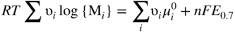
6.3 The Single Potential of an Electrode


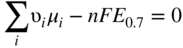
 , Eq. 6.8 can be put into the form
Molten salt
Temperature (°C)
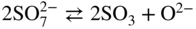
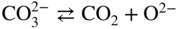
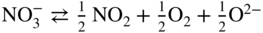
Equilibrium reaction
pO2−
KCl–LiCl, KCl
800

(Na, Li, K)2SO4
600
(Na, Li, K)2CO3
600

(Na, K)NO3
250
 has the following value in terms of the standard chemical potentials of the reactants:
 is the single potential of the electrode measured when the activity of every constituent is equal to unity and is known as the normal or standard potential. Once the normal electrode potential on the standard reference scale is known, the Nernst equation allows a calculation of what the equilibrium electrode potential will be when the system has any {Mi} ≠ 1. Extensive analytical treatments of this subject are given by Conway (1965), de Groot (1951), Grahame (1947), Guggenheim (1929), Parsons (1954), and Prigogine (1947). Experimental proof of the validity of the Nernst equation in molten media is given by Blander et al. (1959), Duke and Garfinkel (1961), Gordon (1899), Ranford and Flengas (1965), and many other workers.
6.4 Equilibrium Diagrams
 ) on the basis of the Lux–Flood regulation (Flood and Förland 1947; Lux 1939) (see also Section 3.3.1). It is recognized that each molten salt has an appropriate acid–base equilibrium involving its anion in the case of the oxyanion system. For example, the basicity expressed as the logarithm
  , assuming an acid–base equilibrium in the alkali sulfate melt:
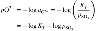
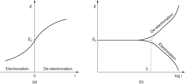
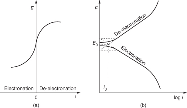
6.5 The Tafel Relationship
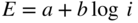

6.6 Corrosion Potential–pO2− Relationship
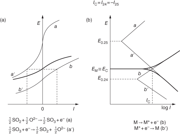
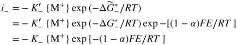
 is the activation energy required for the electronation process at the potential E, K− and
  are constants, {M+} is the activity of cations M+ on the metal side of the interface,
  is the chemical activation free energy barrier when there is zero electric field acting on the ion, and α is the transfer coefficient for the de‐electronation reaction introduced by Erdey‐Gruz and Volmer (1930) that has values ranging from zero to unity (0 < α < 1) (Vetter 1952). K− is dependent on the reference potential chosen since
 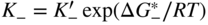 . Moreover, positive ions can move from the melt to the electrode and also in the opposite direction. Thus, there is an electronation reaction

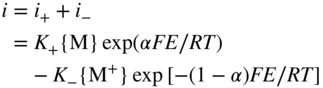
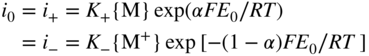

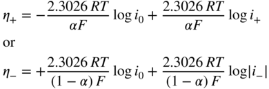
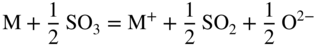

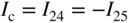
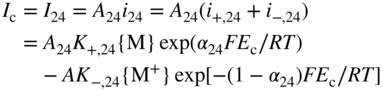
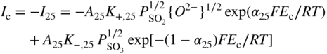
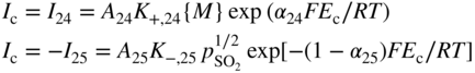
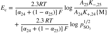
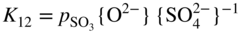
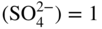 , it follows that
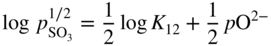
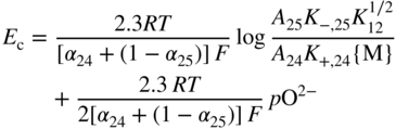
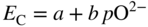
6.7 Electrochemical Polarization and Monitoring
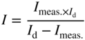
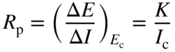
6.8 Electrochemical Nature of Metal Oxidation
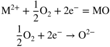
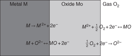

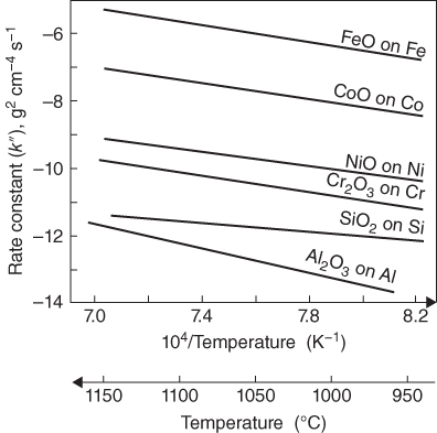


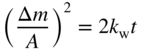
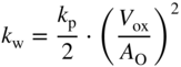
 :
:
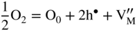
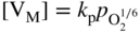
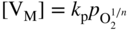
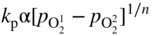
 and
and  are the oxygen partial pressures at the oxide–gas and metal–oxide interfaces, respectively. As the partial pressure of oxygen is strongly decreased at the metal–oxide interface, it can be neglected. Thus, Eq. 6.54 can be written as
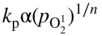
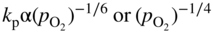
6.9 Usefulness of Electrochemical Cells
Cell type
Measurement technique
Technological application
Polarization cell
Measurement of kinetic data by polarization
Electrochemical composition actors (electrolyzers, pumps, electrochromic windows), electrochemical composition sensors (amperometric, conductometric)
Current‐generating cell
Measurement of kinetic data by depolarization
Electrochemical energy storage and conversion devices (batteries, fuel cells, supercapacitors)
Open‐circuit cell
Measurement of thermodynamic formation data, transport number of electrons
Potentiometric composition sensors
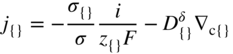
Cell
Quantities to be determined
(O2−, e−|MO|e−, O2−)
Resistances and capacitances
(O2−, e−|MO|e−, O2−) a
Transport numbers, chemical diffusion coefficients
(O2−, e−|MO|e−)
Electronic conductivities as a function of activity, chemical diffusion coefficients
(e−|MO|e−)
Electronic conductivities, chemical diffusion coefficients
(O2−, e−|MO|O2−)
Ionic conductivities as a function of activity, chemical diffusion coefficients
(O2−|MO|O2−)
Ionic conductivities, chemical diffusion coefficients
(O2−|MO|e−)
Stoichiometry, thermodynamic factor, chemical diffusion coefficients
 denoting a missing O2−) and electrons are present and then also associates such as
  (one electron trapped by an oxygen vacancy) and
  (two electrons trapped by an oxygen vacancy), the flux and conductivities in Eq. 6.56 address the total oxygen ensemble,
  (
( does not contribute being effectively neutral). The ensemble diffusion coefficient
  is essentially composed of
  and
and  , as well as of respective differential trapping factors. Of course, interaction can also formally be put on Onsager’s cross coefficient, but this does not provide any mechanistic insight (Onsager 1931).
6.10 Current–Potential Measurements on Solid Electrodes

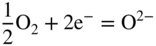
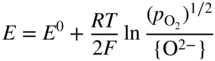
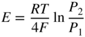

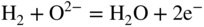
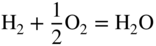
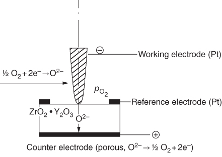
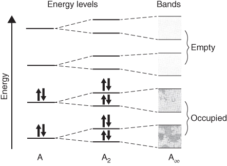
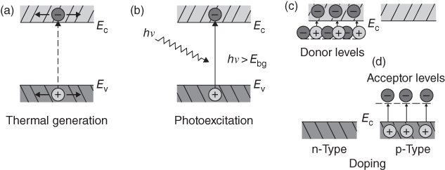
6.11 Simple Concepts of Oxide Semiconductors
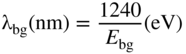
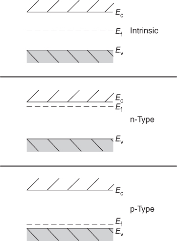
 , i.e. the Fermi levels of the two electrodes match in energy. Now if the semiconductor electrode is biased (by means of a battery or a potentiostat) at a potential one volt positive with respect to the reference electrode, the Fermi level of the semiconductor shifts down in energy with respect to the reference Fermi level. The downward shift arises from the lower energy of electrons in a region of more positive (less negative) potential. Furthermore, the energy difference between the Fermi levels (
 ) is exactly one electron volt (by definition). Biasing the semiconductor negative raises the semiconductor Fermi level above the reference Fermi level. Thus, it is possible to control the semiconductor Fermi level with respect to solution energy levels by means of the applied potential. In the bulk of the semiconductor, the Fermi level remains fixed relative to Ec and Eν, but the situation is different near the electrolyte interface.
6.12 Conduction Processes in Ionic Oxides
 is a metal vacancy singly negatively charged relative to the lattice, and
  is an oxygen vacancy doubly positively charged relative to the lattice. Concentrations of holes or electrons are denoted by p or n, respectively.

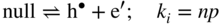

 regions in which the ENC can be approximated by a pairwise equality between two defects. The strength of this method lies in its application to practical situations where, over wide
  regions, there are generally orders of magnitude differences between the concentrations of a predominant defect pair and the minority defects.
 . In this situation
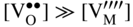

 goes down, k1 requires that
  increase. In turn, this increase requires, through the Schöttky constant ks, that
  decrease, thus leaving e′ and
  as the two negatively charged species. Eventually, the concentration of oxygen vacancies exceeds that of
  , which is fixed by the dopant level, and electrical neutrality must be maintained by increasing n. The intrinsic electronic equilibrium requires p to decrease as n increases.
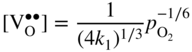
 , there is the same pressure dependence for the electrons, their concentration being just twice that of the oxygen vacancies. Using the Schöttky equilibrium, the
  dependence of the metal vacancy concentration is
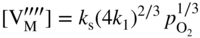
 dependence of the hole concentration.
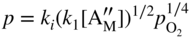
 is determined solely by the Schöttky constant and the oxygen vacancy concentration. At some sufficiently high
  , it is then possible to approximate the ENC in the following manner:

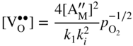
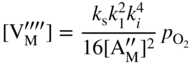

 , the situation occurs where
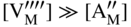
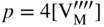
 pressure region, the various defect concentrations are described by
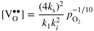
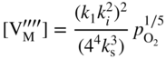
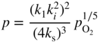
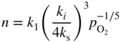
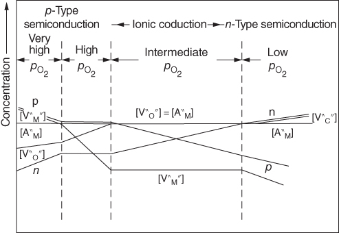
 for an oxide solid electrolyte (logarithmic scale).
 range, the majority defect is ionic, and the concentrations of electronic defects can be substantially depressed below the level of majority defect. If the mobility of the ionic defect is sufficiently high, then it would be expected that the conduction process in the intermediate pressure range would be primarily ionic in nature.
6.12.1 General Partial Current Density

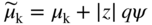
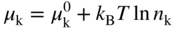
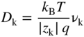
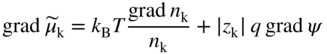

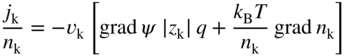
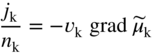
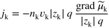
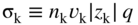
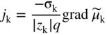
6.12.2 Electronic Current Density
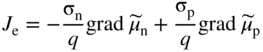
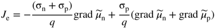

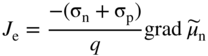
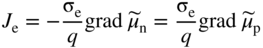
6.12.3 Ionic Current Density

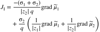
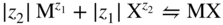
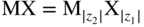 . Equilibrium requires that


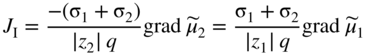
6.12.4 Total Current Density
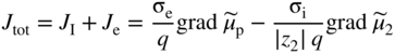
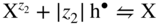
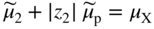
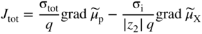
6.13 Common Solid‐State Electrochemical Situations
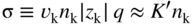

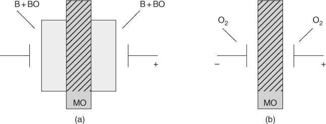
6.13.1 Ohmic Contacts with a Current Supply
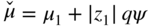
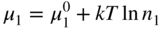
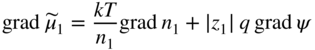

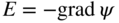
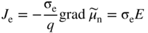
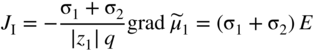
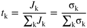
 .
.
6.13.2 Ohmic Contacts with no Current Supply
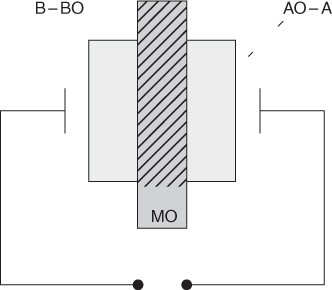
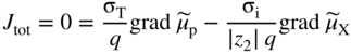
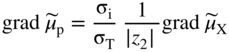
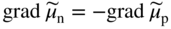
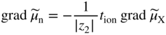

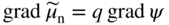
 , and integrating between the boundaries, we have
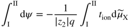
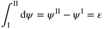
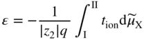
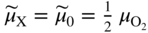 , we arrive at the well‐known equation of Wagner (1935) for electrolytes of mixed conduction:
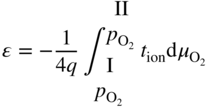
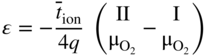
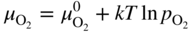
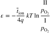
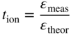
6.13.3 Blocking or Polarizing Electrodes
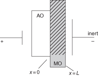
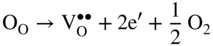
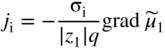
 . As such, the steady‐state current is given by the sum of the partial current densities of the holes and electrons:
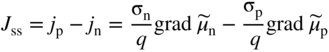
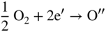
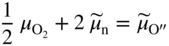
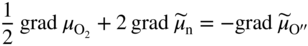
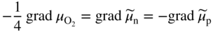
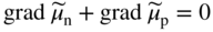
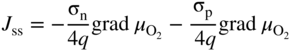
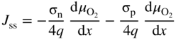
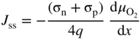
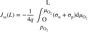
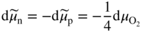
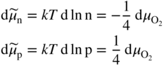
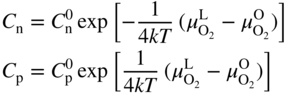
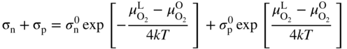
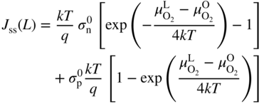
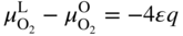
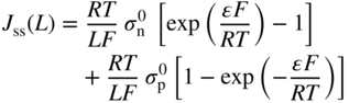


 and
and  are the partial electron and hole conductivities that are defined for the oxide when it is equilibrated with an oxygen chemical potential defined by the reversible electrode. A polarizing electrode technique allows us to measure the partial electrical conductivities directly and, for the case of tion > 0.99, avoids the necessity of taking the difference between two large numbers to arrive at a value for the low‐level electronic contribution to the total conductivity.
References
Further Reading
High Temperature Electrochemistry
6.1
6.3
6.4
6.5
6.6
6.7
6.8
6.9
6.10
6.11
6.12
6.14
6.15
6.16
6.17
6.18
6.19
6.20
6.21
6.22
6.23
6.24
6.25
6.26
6.27
6.28
6.29
6.30
6.31
6.32
6.33
6.34
6.35
6.36
6.37
6.38
6.39
6.40
6.41
6.42
6.43
6.44
6.45
6.46
6.47
6.48
6.49
6.50
6.51
6.52
6.53
6.54
6.55
6.56
6.57
6.58
6.59
6.60
6.61
6.62
6.63
6.64
6.65
6.66
6.67
6.68
6.69
6.70
6.71
6.72
6.73
6.74
6.75
6.76
6.77
6.78
6.79
6.80
6.81
6.82
6.83
6.84
6.85
6.86
6.87
6.88
6.89
6.90
6.91
6.92
6.93
6.94
6.95
6.96
6.97
6.98
6.99
6.100
6.101
6.102
6.103
6.104
6.105
6.106
6.107
6.108
6.109
6.110
6.111
6.112
6.113
6.114
6.115
6.116
6.117
6.118
6.119
6.120
6.121
6.122
6.123
6.124
6.125
6.126
6.127
6.128
6.129
6.130
6.131
6.132
6.133
6.134
6.135
6.136
6.137
6.138
6.139
6.140
6.141
6.142
6.143
6.144
6.145
6.146
6.147
6.148
6.149
6.150
6.151
6.152
6.153
6.154
6.155
6.156
6.157
6.158
6.159
6.160