Zhichao Chen1, Hao Wang1, Yiran Ma1, Cheng Qiu1, Le Yao2, Xinmin Zhang1, and Zhihuan Song1 1Zhejiang University, College of Control Science and Engineering, State Key Laboratory of Industrial Control Technology, 38 Zheda Rd. (Yuquan Campus), Hangzhou, Zhejiang Province, 310027, P. R. China 2Hangzhou Normal University, School of Mathematics, 2318 Yuhangtang Rd., Hangzhou, Zhejiang Province, 311121, P. R. China Inferential sensors are pivotal in process automation, significantly contributing to areas such as modeling, control, and optimization [1, 2]. Their relevance extends across various dimensions of the process industry. One critical aspect involves addressing the demanding challenges of boosting profitability, reducing material usage, enhancing safety, and safeguarding the environment, which has spurred the extensive adoption of artificial intelligence methods, especially deep learning (DL). Concurrently, the escalation in the scale of process manufacturing has intensified the necessity for efficient management of substantial industrial big data volumes [3]. Consequently, the integration of DL techniques into inferential sensors is imperative, aimed at facilitating precise control and optimal decision-making in the realm of process industries. In recent decades, the field of data-driven inferential sensor modeling, especially those methods driven by DL, has seen substantial research and development, fueled by advancements in machine learning algorithms, distributed control systems, and database technologies [1]. DL-based inferential sensor techniques can be classified into several distinct model architectures: (stacked-)autoencoders (SAEs)/feedforward neural networks (FNNs) [4], convolutional neural networks (CNNs) [5], recurrent neural networks (RNNs), and transformers. Each architecture presents its own set of unique advantages and disadvantages. For example, SAEs/FNNs excel in handling process nonlinearity but are less effective with dynamic data. CNNs, with their convolutional kernel structure, offer local memory capabilities but are limited by the predefined size of their receptive field. RNNs adeptly manage dynamic processes [6], yet they are prone to issues like gradient explosion or vanishing during the training phase [7]. Transformers, employing self-attention mechanisms (SAMs), greatly enhance parallelization in sequence modeling, but their inherent “position-insensitivity” due to this mechanism can be a drawback [8]. This diversity among models ensures a well-rounded strategy in addressing the various challenges encountered in inferential sensor modeling. Despite the significant strides made by current DL-based inferential sensor modeling approaches, a critical question persists: How can we effectively integrate established knowledge of industrial processes with these DL models? Industrial processes are subject to stringent evaluation before operation, leading to data that often conforms to empirical rules specific to areas like unit operations and reaction engineering. Incorporating this well-established knowledge into DL models holds the potential to greatly improve their efficacy and relevance. However, unlike physically informed neural networks (PINNs) [9], which model industrial processes at the transport process scale, current inferential sensor-based models, which model processes at unit operation scale, often lack the capability to capture all the necessary coefficients in semi-empirical equations. For instance, the accurate computation in applications such as an absorber column critically depends on the knowledge of mass transport coefficients. However, these coefficients are typically not obtainable through standard instrumentation, resulting in a gap in the necessary data. This chapter categorizes this gap as “incomplete knowledge”. One of the primary challenges we face is the effective articulation and incorporation of this incomplete knowledge into data-driven methodologies. Doing so is essential for improving the performance of inferential sensors. This integration demands not only a deep understanding of the underlying industrial processes but also innovative strategies to compensate for the missing information in a way that enhances the overall efficacy of the inferential sensor models. Recent research increasingly adopts graph neural networks (GNNs) to encapsulate prior knowledge in industrial processes [10–13]. This approach leverages the concept that industrial processes can be graphically represented, with instruments functioning as nodes within this framework. Such a configuration significantly enhances modeling efficacy by enforcing interconnections among various instruments. This methodology mirrors the principles used in recommender systems, where modeling user-item pairs leads to performance improvements [14]. However, this direct adoption of predefined graphs can encounter the following specific challenges: To address the first issue effectively, it is advised to incorporate prior knowledge dynamically within the prior term of the loss function, and subsequently exclude it during the model’s inference stage. This approach contrasts with the conventional method of statically embedding prior knowledge into the model’s input graph and maintaining it throughout the inference stage. Addressing the second issue involves designing a model that inherently and seamlessly adjusts to the evolving prior knowledge. In response to these challenges, this chapter introduces the “variational inference over graph” module, a novel approach designed to adeptly handle both data shifting and knowledge selection in dynamic modeling environments. This chapter is organized as follows: We begin with a comprehensive review of the relevant literature, identifying and discussing the existing technical gaps in the field. Then, in Section 7.3, we delve into the derivation of our proposed methodology, thoroughly detailing the architecture of the innovative module we introduce. Following this, Section 7.4 is dedicated to the empirical validation of our approach, showcasing its application and effectiveness in a real-world catalytic shift unit. The chapter concludes with Section 7.5, where we summarize our key findings and offer insights derived from our research. This chapter is derived from the works of Chen et al. [16, 17]. The integration of prior knowledge into industrial process modeling to enhance model performance is a well-explored domain in data-driven approaches specific to industrial processes. Unlike other fields, industrial processes are subject to rigorous design and rating protocols before they begin operation. This results in process measurement data that generally conforms to established (semi)empirical guidelines, facilitating the seamless integration of prior knowledge into inferential models for industrial process data. In Sections 7.2.1 and 7.2.2, this chapter will be divided into two main areas for detailed discussion: the transport process scale and the unit operation scale, each offering unique insights into the application of prior knowledge in industrial process modeling. In the realm of transport processes, industrial operations are governed by well-established conservation laws of momentum, heat, and mass. Reflecting this foundation, PINNs, which replace nonlinear terms in partial differential equations (PDEs) or ordinary differential equations (ODEs) with neural networks, have gained substantial attention in recent research, as highlighted in works by Raissi et al. [18] and Zhiyong et al. [19]. A prominent example is in the prediction of turbulent flows, where Wang et al. [20] developed the turbulent-flow net, integrating trainable spectral filters with Reynolds-averaged Navier–Stokes equations and large Eddy simulation in a specialized U-net structure. Addressing few-shot learning challenges, Zheng et al. [21] proposed a physics-informed RNN within a model predictive control framework, ensuring compliance with physical laws while substituting key equations with an RNN. While PINN-based models have found considerable application in process control, as noted by Alhajeri et al. [22] and Zheng et al. [21], their direct application using process measurement data in PINNs faces challenges due to the complex transport phenomena in unit operations. This complexity limits the broader application of PINN-based methods in industrial process inferential sensors. At the unit operation scale, practitioners typically use graph structures rather than strict ODE/PDE formulations to represent process knowledge. In this context, Bayesian networks (BNs), as discussed by Zeng et al. [23] and Khosbayar et al. [24], are a natural choice for modeling the correlations between process variables. Khosbayar et al. [24], for instance, designed BN structures based on flowsheets, developed a corresponding parameter estimation algorithm using the expectation–maximization algorithm, and validated its effectiveness in a bitumen upgrading process. However, the training and inference of BNs, typically based on the expectation propagation algorithm, are not easily integrated into the mini-batch stochastic gradient descent-based DL framework. To address this, recent studies have increasingly focused on GNN-based models [11, 12, 25]. Notably, Ren et al. [12] used normalized mutual information to extract the graph of process variables, applied a multi-level knowledge graph to model large-scale industrial process data, and demonstrated its effectiveness in a cobalt–nickel removal process. Despite significant advancements in embedding prior knowledge in industrial process inferential sensors, the following key issues remain unresolved: To bridge these identified technical gaps, we introduce the variational inference over graph (VIOG) framework in Section 7.3. In this section, our approach begins by reinterpreting the graph within a Bayesian framework and modifying the loss function to include graph constraints, thereby addressing the “data shifting problem” issue. Next, we consider the knowledge representation problem in detail. Specifically, we examine the process of information selection among various variables, leading to the development of a SAM aimed at resolving “knowledge selection problem” issue. Additionally, we analyze the parallels between this SAM and graph convolution operations to underscore its validity. The section culminates with the presentation of the overall architectural design of the VIOG framework. De facto, the task of inferential sensing can be regarded as a specific case of a supervised learning task. Consequently, if we represent the process variables by x, the quality variable by y, and the parameters by θ, our learning objective can be articulated as follows: Based on Eq. (7.1), we can reformulate the learning objective as follows: where the third line is built upon the Jessen’s inequality [26, 27]. Besides, we can further divide the last line of Eq. (7.2) and formulate a novel optimization problem as follows: Comparing Eqs. (7.2) and (7.3), it becomes evident that our learning objective transforms the conventional constraint term, typically a constant in most GNN-based models, into a penalty term. This transformation can be understood through the application of the celebrated Lagrangian multiplier method: where β functions as the Lagrangian multiplier, with the learning objective of the β-VAE outlined on the right-hand side of Eq. (7.4). A key innovation within our variational inference framework is the conversion of the standard predefined graph, a common feature in GNN-based models, into a penalty form. This adaptation enables our model to operate without reliance on a specific graph structure, enhancing its versatility. This approach effectively addresses the “data shifting” issue as discussed in Section 7.1. Section 7.3.2 will explore the representation and integration of prior knowledge in our model, further clarifying its significance and operational mechanism. In this subsection, we aim to elucidate the methodology for integrating incomplete knowledge into the prior term Echoing approaches in the natural language processing domain, where sentences are delineated using graph-like grammar trees [28], our model in GNN-based industrial process modeling similarly employs graphs to represent knowledge regarding process covariates. However, as previously mentioned, this prior knowledge is characteristically uncertain. The essence of utilizing this uncertain knowledge effectively lies in its probabilistic representation. Consequently, this subsection is dedicated to introducing an approach for articulating prior knowledge from a probabilistic perspective. According to previous works [29, 30], the graph adjacency matrix where ν indicates the unique element number of the process variables. In light of this, the edges (denoted as α) in the graph may be present (α = 1) or absent (α = 0). This phenomenon indicates that the Bernoulli distribution can be adopted to describe the edges’ state as Eq. (7.6) shown: where ρ represents the expected value of the Bernoulli distribution. Given our comprehension of the process, knowledge can be classified into three discrete states: definitively present, ambiguously present, and definitively absent. To address this, we employ the 2σ bound within the Gaussian distribution, following the Pauta criterion, to determine the value of ρ. This method enables us to formulate the subsequent disjunctive expression: where ⊻ indicates that only one square bracket will take effect. Having delineated our prior graph In summary, based on our analysis, the following design requirements are essential to address the “knowledge selection” issue: To address requirement (1), we can conduct similarity measurement as follows: where Here, sij denotes an element of the matrix The abovementioned graph construction is similar to the SAM [32] in the transformer model as depicted in Figure 7.1. In the next part, we want to discuss the similarity between the GNN and transformer model. In Section 7.3.2.3, our primary focus lies in the comprehensive examination of the similarities between GNN-based networks and transformer models. For simplicity, we consider graph CNNs, the most widely used in the process industry, as an analysis object. It is worth emphasizing, as articulated in the scholarly reference [33], that the GNN exhibits distinct characteristics within the realm of message passing neural networks, as explicitly elucidated in Eq. (7.11): where the symbol φ represents an operator that transforms the features of node i and those from its neighboring nodes j into a single, unified message. Concurrently, ζ denotes a permutation-invariant operator responsible for aggregating all messages associated with node i. This aggregation can be executed through various methods, such as summation, mean calculation, or maximization. Finally, the γ operator is employed to map the features of node i onto the aggregated message generated by the ζ operator, effectively integrating node-specific information with broader network insights. As such, the feature at node i in the kth GC layer is obtained: Figure 7.1 Model Structure of (a) transformer Model, (b) SAM, and (c) multi-head SAM. Equation (7.11) can be rewritten as Eq. (7.12) for the GC operator [34], where the U and W are the weights that should be learned, the + is adopted as the γ operator in Eq. (7.11), the ∑ (sum) is chosen to be the ζ operator, and φ operator is linear transformation. Besides, in (7.12), the self-loop (the node i itself is included in the set of its neighboring node ℕ(i)) exists for all nodes. By analyzing Eq. (7.12), the corresponding structure can be drawn as Figure 7.2a shows. Meanwhile, as shown in Figure 7.2b, the SAM [32] can be described as Eq. (7.13) to Eq. (7.15). Equation (7.13) shows that the input data are mapped into the vector space named Q (query), K (key), and V (value), respectively. The similarity for vectors in Q space and K space can be transformed into the weight on vectors in V space, considering the scaling factor D as shown in Eq. (7.14), where the weight is called attention value, and the matrix formed by the attention values is denoted as Figure 7.2 The structure of (a) the message passing of GNN, (b) the self-attention mechanism. This analysis leads to the conclusion that the similarity computation achieved through the inner product and the weighted summation operation, as described in Eq. (7.13), is essentially analogous to the operation of summing the neighboring nodes detailed in Eq. (7.12). In essence, this implies that the SAM can be equated to GC. This equivalence suggests that the attention matrix In Section 7.3.2.3, we conduct a detailed analysis of the reason for introducing SAM and the similarity of SAM and GC operator. Nevertheless, the model training issue remains a challenge; since the loss function is derived within the variational inference framework, where obtaining sample from the posterior distribution is vital to proceed the model training. To this end, the remain of this part will focus on how to obtain samples from the posterior distribution. First, let us review the normalization constraint introduced by SAM: Building on this framework, the distribution of each row in Although the Dirichlet distribution meets these criteria and promotes sparsity, making it an intuitive choice, it poses a challenge in that it is not parameterizable for backends based on gradient descent-driven DL techniques. Consequently, in alignment with the approach suggested in Ref. [35], a strategy is adopted wherein random variables are drawn from a nonnegative distribution and subsequently normalized to adhere to the simplex constraint. This process enables the derivation of the column vector where the subscript i indicates the row vector at row i, and the In this chapter, the log-normal distribution defined in Eq. (7.18) is chosen as the nonnegative distribution, and σ of the log-normal distribution is treated as a global hyperparameter: Since sampling from a log-normal distribution is equivalent to sampling from a normal distribution: Thereby, the unnormalized attention weight Note that the sampling operation ensures Eq. (7.21) set up, which means that the gradient estimation of the unnormalized graph Based on our abovementioned approaches we name our module VIOG, where we use the variational inference framework, and our model can be treated as a special kind of GNN. Besides, we have not introduced the model structure assumption in our derivation process, which indicates that our proposed approach can be a plug-in module and can be adapted to most of the current model structure. On this basis, our proposed model architecture is given as follows: Figure 7.3 presents the illustration of the VIOG, which consists of the VIOG module and downstream DL models. The Bayesian SAM parameterized by φ in the VIOG module serves as Suppose the input tensors are in shape like [batch size, sequence length, ν]. Before all operations, the reshape operation in Eq. (7.22) is first executed to avoid breaking their time–series structure. After that, the linear projection for input tensor embedding on each dimension in shape [batch size × seq length, 1] is conducted as Eq. (7.23): Typically, instead of performing a single attention function, it is beneficial to linearly project the queries, keys, and values H times with different, learned linear transformations. Thereby, (7.23) will execute parallelly in H heads. Thereafter, the similarity sij can be obtained as (7.24): On this basis, where the subscript j signifies that the log-softmax operator (log-softmax) is applied column-wise, specifically targeting the column index j, and executed on a row-by-row basis. As such, the And thus, the nonnegative random variable αij can be obtained as per (7.27): Figure 7.3 The illustrator of the VIOG module. The entity αij of In this procedure, the unnormalized attention weight, instrumental in calculating the KL divergence term, is provided as depicted in (7.29): Note that the inference of the label where h is the hidden feature, and subscript res stands for residual. Besides, to avoid the over-fitting of the VIOG module, it is suggested to adopt the dropout layer after obtaining the final feature hfinal [32, 36]. And finally, the loss function for the DL models with the VIOG module can be rewritten as (7.32): where β acts as a balancing mechanism, harmonizing the trade-off between prediction error and knowledge-based regularization. In this section, the effectiveness of the VIOG module for industrial process inferential sensors will be demonstrated on a catalytic shift conversion (CSC) unit. We devise experiments on an industrial inferential sensor dataset, to verify the superiority of OC–NDPLVM and answer the research questions as follows: The root mean square error (RMSE), coefficient of determination (R2), mean absolute error (MAE), and mean absolute percentage error (MAPE) are leveraged as the evaluation indices. The detailed expressions are given in Eqs. (7.33)–(7.36), respectively. where To showcase the effectiveness of our proposed method, we conduct a case study focusing on quality prediction in a real CSC unit, which belongs to an ammonia synthesis process. In the following content, we offer an in-depth overview of the technical background pertinent to these industrial processes. Figure 7.4 illustrates the process flow diagram of the CSC unit, as described in Ref. [37], which is integral to an actual ammonia synthesis process. The chemical reaction, as specified in Eq. (7.37), occurs within fixed-bed reactors. A critical aspect of ammonia synthesis is maintaining an optimal carbon–hydrogen ratio. This unit comprises two isothermal fixed-bed reactors arranged sequentially. The initial step involves compressing the reactant gas into the first high-temperature reactor, ensuring the achievement of thermodynamic equilibrium and an appropriate reaction rate. Subsequently, the gas is cooled in the second reactor, modifying the equilibrium phase to favor increased hydrogen yield. This process results in a final product gas, ready for further processing in subsequent downstream operations. Given that Eq. (7.37) outlines an exothermic reaction, as detailed in Ref. [38] (where δH indicates the enthalpy change): wherein elevated temperatures may shift the equilibrium toward the reverse reaction. This shift, in accordance with Le Chatelier’s principle, typically results in a decreased conversion rate of carbon monoxide. Conversely, the reaction kinetics, guided by the Arrhenius equation, indicate that the reaction rate is significantly reduced at lower temperatures. Consequently, to optimize the conversion efficiency, it is practical to conduct the reaction using different catalysts at varied temperature ranges. This approach effectively balances the thermodynamic and kinetic considerations, ensuring optimal conversion from both perspectives. The technological specifications previously described necessitate accurate, real-time monitoring of carbon monoxide levels, specifically at the outlet of the low-temperature bed, which is highlighted in green in Figure 7.4. Traditional measurement techniques, such as gas chromatography, however, introduce significant delays in carbon monoxide content detection. To enhance the control of the reactor and enable immediate monitoring of carbon monoxide concentrations, hard sensors have been deployed to gather essential process variables. For the purpose of constructing a robust quality prediction model, 13 key variables have been selected. These variables and their respective roles in the process are elaborately detailed in Table 7.1. Figure 7.4 Flowsheet of CSC unit. Based on the principles of chemical reaction engineering, the reactors are analyzed employing the plug-flow reactor model, as depicted in Figure 7.5. By analyzing the length-l infinitesimal (dV) marked in the white zone, the mass conservation of reactant γ can be derived as shown in (7.38), where ζ is the bed voidage, ℱ is the flow rate, and ℛ is the reaction rate. Table 7.1 Variable of CSC process. Figure 7.5 The plug-flow reactor model. Meanwhile, the heat conservation [39] can be given in (7.39): where Gc indicates gas heat capacity, subscript c is the abbreviation of capacity, and According to Ergun equation, the pressure drop ( where Re is Reynold’s number, ρg is reactant gas density, ug is gas velocity, and subscript g is the abbreviation of “gas.” Note that the gas velocity determines the ratio of gas reactant diffusion rate and reaction rate (also known as Thiele modulus). And thus, in the designing stage of the reactor, the velocity and the voidage should be well designed to make the pressure drop as small as possible for higher reactant conversion [40]. Throughout the analysis of the CSC process, we can have the following prior knowledge: Figure 7.6 (a) The prior knowledge adjacency matrix of CSC; (b) The normalized prior knowledge adjacency matrix of CSC. Consequently, the prior knowledge of the CSC process can be obtained as Figure 7.6a shows, where the prior knowledge part and the diagonal are 0.955, and other elements are 0.045. The normalized graph by log-softmax function by rows is given in Figure 7.6b, which is adopted as the value of μ in the prior log-normal distribution. We choose the following kinds of baseline models to demonstrate the effectiveness of our VIOG module. The hyperparameter setting and other training protocols are reported in Appendix 7.A. To facilitate comprehension, the final column showcases the “win counts” as per Ref. [41], representing the metrics where the model featuring the VIOG module outperforms the baseline models: Table 7.2 presents the evaluation metrics results for different models. The following observations can be obtained: Observation 1 highlights the efficacy and superiority of our proposed VIOG module across most downstream models in industrial data modeling tasks. However, as noted in Observation 2, the VIOG module demonstrates only marginal improvements when compared to other GNN models. This limited enhancement could be attributed to the complexity of the model architecture. For instance, the transformer model, characterized by its larger parameter count and more intricate encoder and layer structure, presents greater optimization challenges compared to other models. Consequently, the VIOG module’s impact on improving the transformer model is less pronounced than it is on other downstream models. Further supporting this, Observation 3 points out the similarity between traffic flow prediction tasks and inferential sensor tasks. In traffic flow predictions, adaptive GNN models such as Graph WaveNet [44], MTGNN [45], and FC–GAGA [46], which can be considered variants of synthesizer-based models [43], align with the findings of Observation 3. Table 7.2 Comparison to baseline models. The VIOG module incorporates a prior knowledge regularization term into its learning objective, a feature that inherently enhances model performance. In this subsection, we aim to conduct a comparative analysis between this prior knowledge-based regularization term and the conventional L1 and L2 regularization terms. This comparison is intended to further demonstrate our method’s superiority. Following the approach used in Section 7.4.5, we implement a grid search for the L1 and L2 regularization terms and present the findings in Table 7.3. From Table 7.3, we found that our VIOG module consistently outperforms conventional L1 and L2 regularization terms across various downstream models. This outcome highlights the effectiveness and superiority of the knowledge regularization term introduced by VIOG. However, it is noted that the prior knowledge regularization term underperforms when applied to LSTM and transformer downstream models within the context of the CSC dataset. This can likely be attributed to reasons analogous to those discussed in Section 7.4.5. Specifically, the CSC unit’s direct connection to downstream production units, which maintains high reactant purity and stable production content at set points, can be equated to “conceptual drift” in machine learning terminology. As a result, the VIOG-augmented downstream model exhibits diminished performance compared to traditional L1 and L2 regularization when tested on the CSC dataset. Nonetheless, in most tested scenarios, the VIOG’s regularization term demonstrably enhances the performance of downstream models beyond what is achieved with standard L1 and L2 terms. This finding emphasizes the broad-scale superiority of the VIOG module in enhancing model performance. Table 7.3 Comparison to baseline models. In this subsection, we conduct a sensitivity analysis of the VIOG model paired with a transformer downstream model, utilizing the CSC dataset. The outcomes of this analysis are depicted in Figure 7.7. Here, we observe how the model’s performance varies with adjustments in regularization strength and batch size. As evident from this figure, despite some fluctuations in performance due to changes in hyperparameters, the model consistently exhibits strong performance. This indicates that the VIOG module is effectively designed, demonstrating resilience across a broad range of hyperparameter settings. Figure 7.7 The sensitivity analysis results on the transformer downstream model of (a) RMSE, (b) R2, (c) MAE, (d) MAPE along batch size for the CSC dataset. The sensitivity analysis results of (e) RMSE, (f) R2, (g) MAE, and (h) MAPE along regularization strength β for the CSC dataset. In this study, we introduced the VIOG module, designed to automatically encode and select knowledge as DL features in data-driven industrial process modeling. The VIOG module enhances traditional DL models by incorporating a VIOG inference network and a novel prior knowledge regularization term. Our approach involved analyzing the probabilistic graph structures inherent in conventional GNNs and DL models. This analysis guided the development of the variational inference technique, which utilizes prior knowledge as a regulatory factor. Furthermore, we crafted the SAM as a unique spatial-based GNN variant, aiming to assimilate prior knowledge effectively. The loss function of the VIOG module was also meticulously derived to align with these objectives. To demonstrate its efficacy, the VIOG module was applied in inferential sensor experiments within the CSC process, where it exhibited superior performance. While the VIOG module shows promising potential, it stands to benefit from advancements in two key areas. First, the computation of attention scores in the VIOG module is computationally demanding, requiring significant time and memory resources. A potential solution lies in adopting sampling techniques similar to those proposed in [41], which could significantly reduce the training costs associated with VIOG. Secondly, there is room for improvement in the precision of data probabilistic density estimation. The current reliance of the VIOG module on amortized variational inference techniques leads to what is known as an “amortization gap” – a discrepancy between the log-likelihood and the evidence lower bound (ELBO) as detailed in [50]. This gap might be narrowed by integrating variational inference with importance sampling methods, enhancing the tightness of the ELBO, a concept explored in [51]. For simplicity, we set the regularization strength β of the VIOG module as 1.0. We conduct grid search on learning rate in [0.0001, 0.001, 0.01, 0.1, 1.0] and batch size in [32, 64, 128, 256, 512, 1024]. For L1 and L2 regularization terms, we select the model regularization strength as 0.001 by applying grid search in [0.001, 0.005, 0.010, 0.020]. The learning rate and batch size adopted in models are listed in Table 7.A.1. Other hyperparameters are listed as follows: In addition, both GCN and GAT necessitate a predefined graph structure during the model inference phase. To address this requirement, we consider the existence of edges in the prior graph as being governed by a Bernoulli distribution. Following this approach, the edges of the graph are independently sampled from their respective Bernoulli distributions, aligning with the mean-field assumption on graphs as outlined in Ref. [30]. We organize the dataset in ascending order based on timestamps. Subsequently, we allocated the first 60% of the data for training purposes, the subsequent 10% (from 60% to 70%) for validation, and the remaining portion for testing. For model optimization, we employ the Adam optimizer, as outlined in [52]. All experimental procedures are performed on a high-specification workstation equipped with four Intel Xeon E5 processors, eight NVIDIA GTX 1080 graphics cards, and 128 GB of RAM. The model training and inference processes are conducted using Python 3.8, with PyTorch 1.10 [53] serving as the DL backend. To ensure robustness and reduce randomness in our results, each experiment is replicated a minimum of three times, each time using one of seven distinct random seeds. Table 7.A.1 Hyperparameters of the CSC dataset.
7
Integrating Incomplete Prior Knowledge into Data-Driven Inferential Sensor Models Under Variational Bayesian Framework
7.1 Introduction
7.2 Literature Review
7.2.1 Transport Process Scale
7.2.2 Unit Operation Scale
7.2.3 Overall Summary and Technical Gap
7.3 Proposed Approach
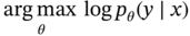
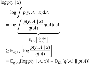
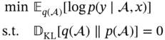
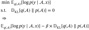
7.3.1 Loss Function Derivation
7.3.2 Knowledge Representation
 (knowledge description) and to outline the framework for such a representation within our model (knowledge utilization).
7.3.2.1 Knowledge Description
 can be decomposed using the mean-field assumption:
7.3.2.2 Knowledge Section via Self-Attention Mechanism
 , our focus now shifts to the variational distribution
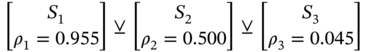
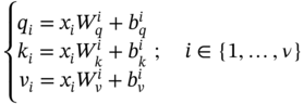
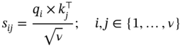
  . In line with existing literature, graph construction hinges on nodal similarity, which, in our case, translates to the similarity among different process variables. However, solely measuring node similarity is insufficient to tackle the problem of knowledge selection. For instance, consider a source node denoted by i ∈ {1, 2, …, ν} and a target node represented as j ∈ {1, 2, …, ν}. Each target node j might receive input from ν source nodes, potentially leading to redundant information. Therefore, it is imperative to implement a competitive mechanism. This mechanism should not only limit the information received by the target node j but also regulate the information emitted from the source node i.

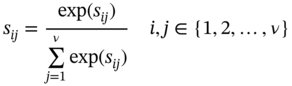
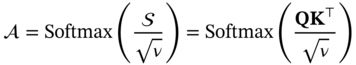
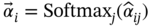
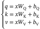
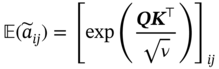
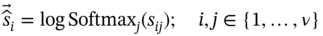
 , Q, and K represent the similarity matrix, the information from the source, and target nodes, respectively. To impose restrictions on this information, we employ a row-by-row normalization using the softmax operator:
 . It is important to note that directly applying a competitive approach to a matrix
  could lead to a “winner takes all” scenario, where the rows of the matrix
  transform into one-hot vectors. Such an occurrence could complicate the model training process and induce significant variance during the gradient estimation phase [31]. To mitigate these issues, the matrix
  is derived from
  :
:
7.3.2.3 Similarity of GCN and SAM
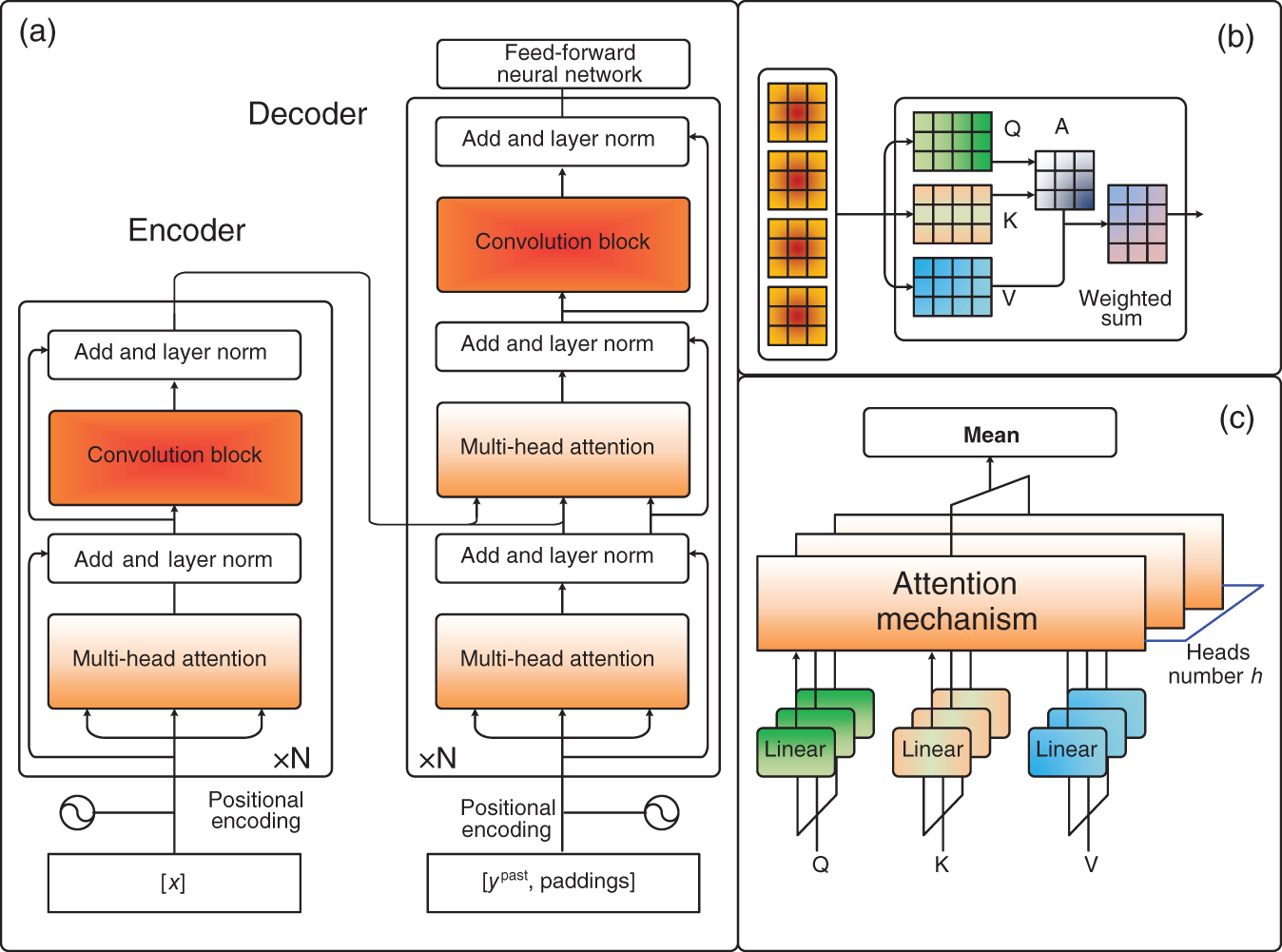
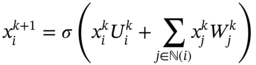
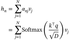
 . Equation (7.15) stands for the residual block which means that the final output is the sum of the original input data x and the h vector obtained from Eq. (7.14).
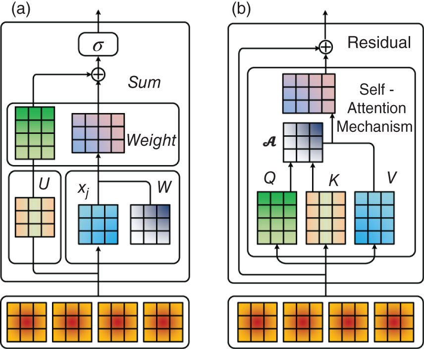
 , derived through SAM, can represent the interconnections between different nodes in the network. The process of obtaining this attention matrix can thus be viewed as a data-driven approach to knowledge discovery. Based on these insights, it becomes feasible to design our model architecture with a foundation in SAM.
7.3.2.4 Sampling from Posterior
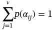
 is subject to certain constraints, specifically:
 for the attention matrix or graph
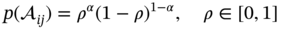
  , as delineated in Eq. (7.6):
 is a random sample drawn from a nonnegative distribution.

 can be obtained via the expected value μ of the normal distribution, and the expected value μ can be obtained as Eq. (7.20):
 (the entity is denoted as
  ) is unbiased:
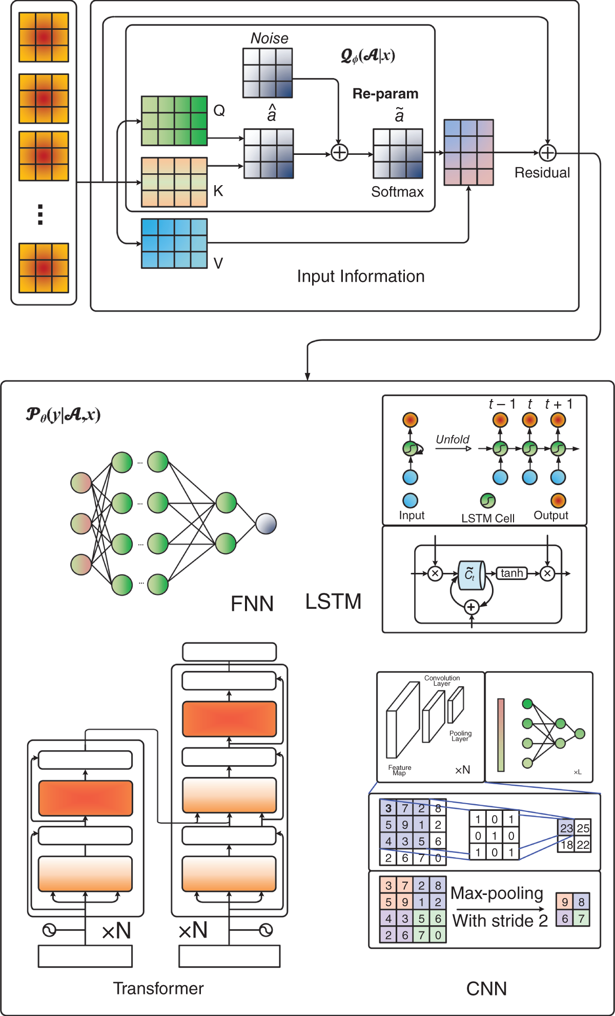
7.3.3 Model Expressions
 , which undertakes the task of leveraging and reconciling the prior knowledge. While the DL models are parameterized by θ serve as
  support tasks like soft sensors and process monitoring.
 is calculated row-by-row as (7.25):
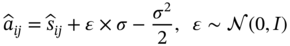
 is reparametrized with noise sampled from
  as per (7.20):
 is obtained via row-by-row normalization as per (7.17). It is worth noting that (7.27) and (7.17) are functionally equivalent to the softmax operation:
 is conditioned on A and x. While the abovementioned description mainly concentrates on
 . To include the information of x, the weighted sum in (7.30) and residual operations (7.31) similar to the SAM is also indispensable:
7.4 Experimental Results
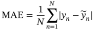
7.4.1 Evaluation Metrics
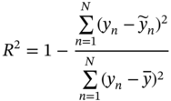
 is the mean value of the label,
  is the predicted value, y is the real value, and N is the data number of the testing dataset. For RMSE, MAE, and MAPE, the smaller value, the more accurate the model. On the contrary, the closer R2 to 1, the better the model fits.
7.4.2 Process Description
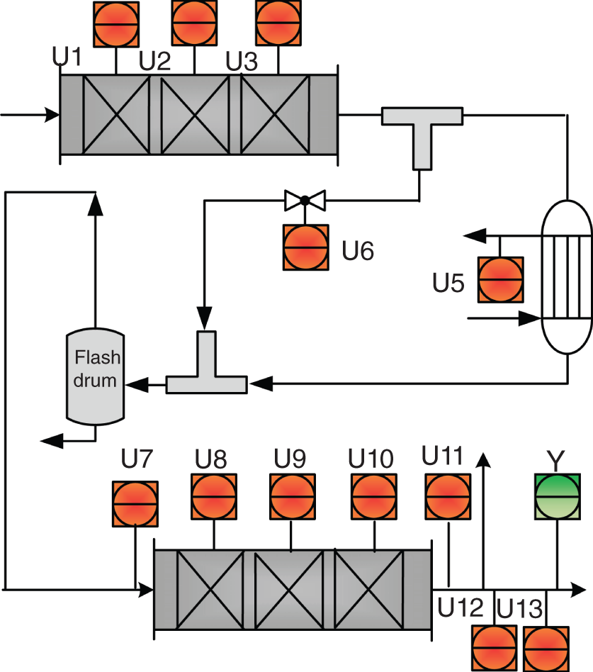
7.4.3 Prior Knowledge Analysis
Variable
Description
U1
High-temperature bed, temperature 1
U2
High-temperature bed, temperature 2
U3
High-temperature bed, temperature 3
U4
Outlet temperature of high-temperature bed
U5
Outlet temperature of cooling water
U6
Split-gas temperature
U7
Inlet temperature of low-temperature bed
U8
Low-temperature bed temperature 1
U9
Low-temperature bed temperature 2
U10
Low-temperature bed temperature 3
U11
Outlet temperature of low-temperature bed
U12
Outlet pressure of low-temperature bed
U13
Product gas pressure
Y
Carbon monoxide concentration 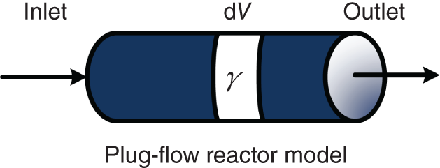
 indicates temperature.
 ) can be derived as follows:
7.4.4 Baseline Models
7.4.5 Model Performance Comparisons
Structure
RMSE
R2
MAPE
MAE
VIOG
0.144 ± 2.414 × E-6
0.939 ± 3.986 × E-6
0.058 ± 5.842 × E-7
0.114 ± 2.249 × E-6
GCN
0.161 ± 9.606 × E-5
0.904 ± 2.689 × E-4
0.065 ± 1.614 × E-5
0.127 ± 6.230 × E-5
GAT
0.179 ± 9.385 × E-4
0.877 ± 4.352 × E-3
0.069 ± 1.340 × E-4
0.137 ± 4.929 × E-4
SynDense
0.174 ± 4.127 × E-4
0.898 ± 7.115 × E-4
0.069 ± 5.540 × E-5
0.135 ± 2.136 × E-4
SynRandom
0.147 ± 3.648 × E-5
0.934 ± 6.423 × E-5
0.059 ± 7.612 × E-6
0.116 ± 2.933 × E-5
SVAE
0.159 ± 1.997 × E-5
0.928 ± 1.681 × E-5
0.064 ± 2.517 × E-6
0.125 ± 9.625 × E-6
ANP
0.239 ± 2.121 × E-4
0.836 ± 4.134 × E-4
0.096 ± 3.981 × E-5
0.188 ± 1.537 × E-4
7.4.6 Comparison with L1 and L2 Regularization Terms
Downstream
Regularization
RMSE
R2
MAPE
MAE
FNN
VIOG
0.144 ± 2.414 × E-6
0.939 ± 3.986 × E-6
0.058 ± 5.842 × E-7
0.114 ± 2.249 × E-6
L1
0.177 ± 2.043 × E-4
0.907 ± 1.656 × E-4
0.070 ± 3.487 × E-5
0.128 ± 5.882 × E-4
L2
0.188 ± 1.171 × E-4
0.908 ± 1.563 × E-4
0.075 ± 1.481 × E-5
0.147 ± 5.726 × E-5
CNN
VIOG
0.143 ± 3.583 × E-5
0.934 ± 8.610 × E-5
0.057 ± 5.353 × E-6
0.112 ± 2.048 × E-5
L1
0.147 ± 4.017 × E-5
0.931 ± 8.462 × E-5
0.058 ± 5.514 × E-6
0.115 ± 2.122 × E-5
L2
0.151 ± 1.104 × E-4
0.928 ± 9.043 × E-5
0.060 ± 1.616 × E-5
0.118 ± 6.235 × E-5
LSTM
VIOG
0.150 ± 5.858 × E-5
0.921 ± 1.965 × E-4
0.060 ± 9.164 × E-6
0.117 ± 3.531 × E-5
L1
0.145 ± 3.775 × E-5
0.930 ± 9.769 × E-5
0.058 ± 5.670 × E-6
0.113 ± 2.194 × E-5
L2
0.149 ± 4.249 × E-5
0.924 ± 1.376 × E-4
0.059 ± 5.456 × E-6
0.116 ± 2.102 × E-5
Transformer
VIOG
0.173 ± 8.454 × E-5
0.906 ± 1.676 × E-4
0.0692 ± 1.426 × E-5
0.1361 ± 5.497 × E-5
L1
0.180 ± 3.464 × E-4
0.890 ± 1.211 × E-3
0.0737 ± 6.530 × E-5
0.1425 ± 2.508 × E-4
L2
0.172 ± 3.250 × E-4
0.902 ± 8.558 × E-4
0.0694 ± 5.509 × E-5
0.1364 ± 2.117 × E-4
7.4.7 Sensitivity Analysis

7.5 Conclusions
Experimental Settings
batch
Lr
Structure
FNN
CNN
LSTM
Transformer
FNN
CNN
LSTM
Transformer
VIOG
1024
64
64
32
0.01
0.001
0.001
0.005
GCN
1024
64
64
32
0.01
0.001
0.001
0.005
GAT
1024
64
64
32
0.01
0.001
0.001
0.005
SynDense
1024
64
256
64
0.01
0.001
0.001
0.001
SynRandom
1024
128
256
1024
0.01
0.01
0.001
0.001
SVAE
32
256
512
1024
0.01
0.01
0.01
0.01
ANP
128
64
64
32
0.01
0.01
0.01
0.01
L1
1024
64
64
32
0.01
0.001
0.001
0.005
L2
1024
64
64
32
0.01
0.001
0.001
0.005
References
Integrating Incomplete Prior Knowledge into Data-Driven Inferential Sensor Models Under Variational Bayesian Framework
(7.5)
(7.7)
(7.8)
(7.9)
(7.10)

(7.16)
(7.19)

(7.26)
(7.28)

(7.34)
(7.35)


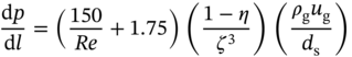
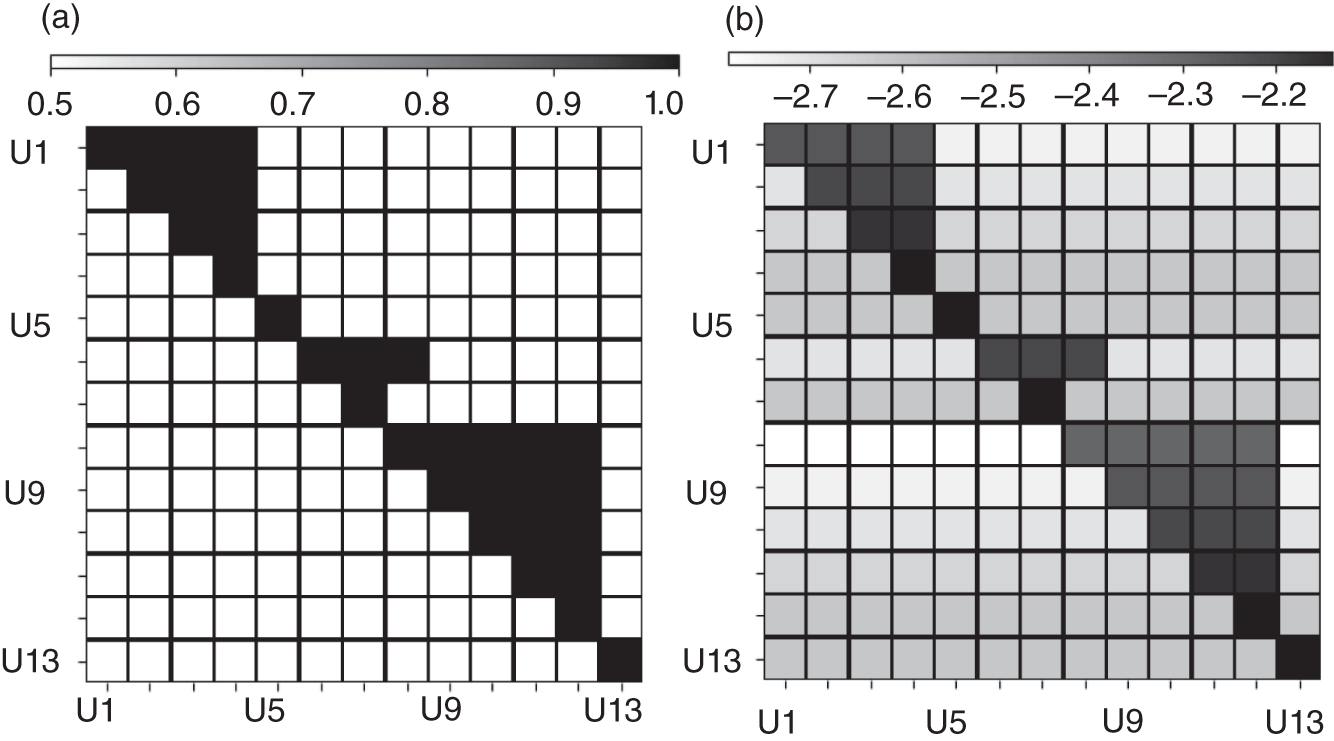
(7.40)