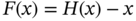
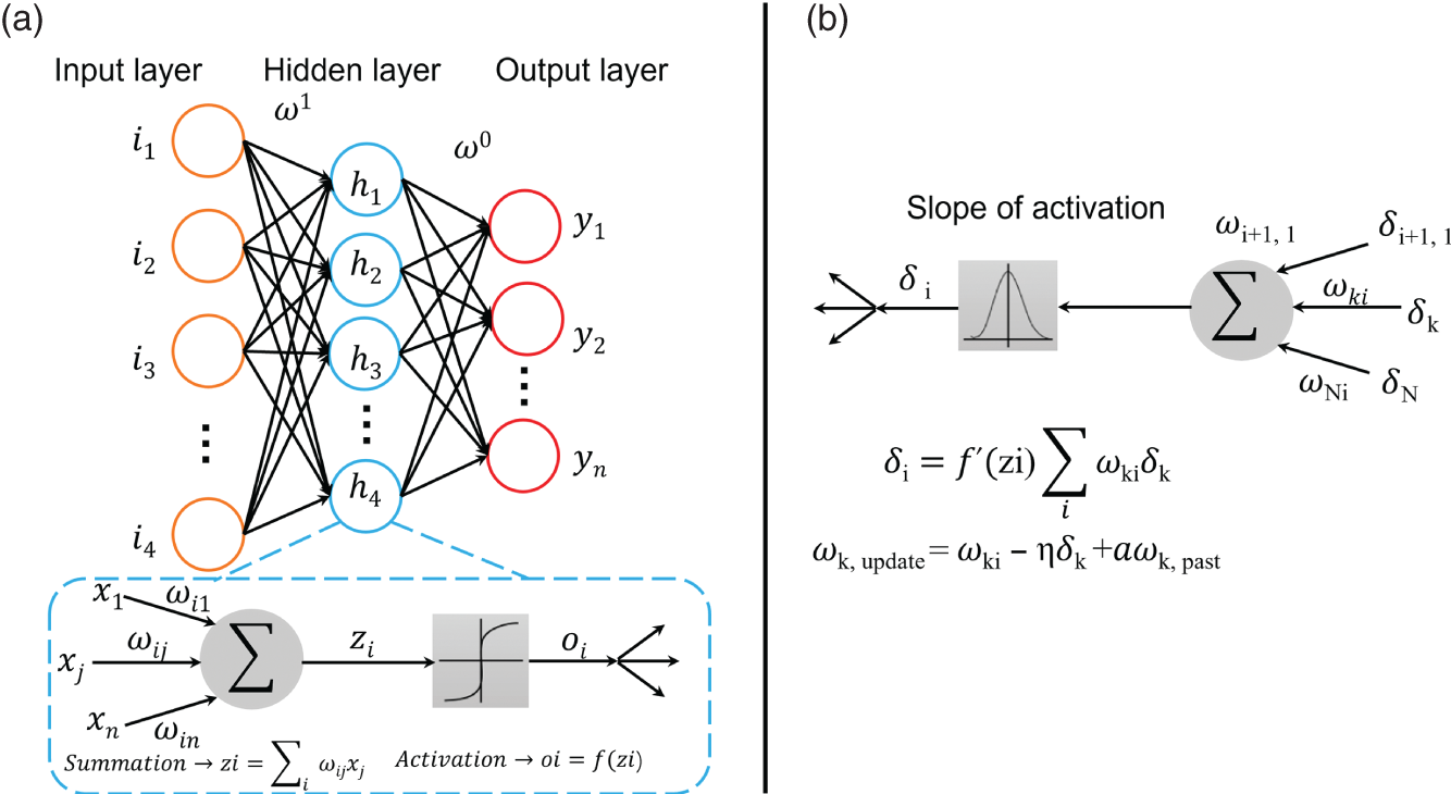
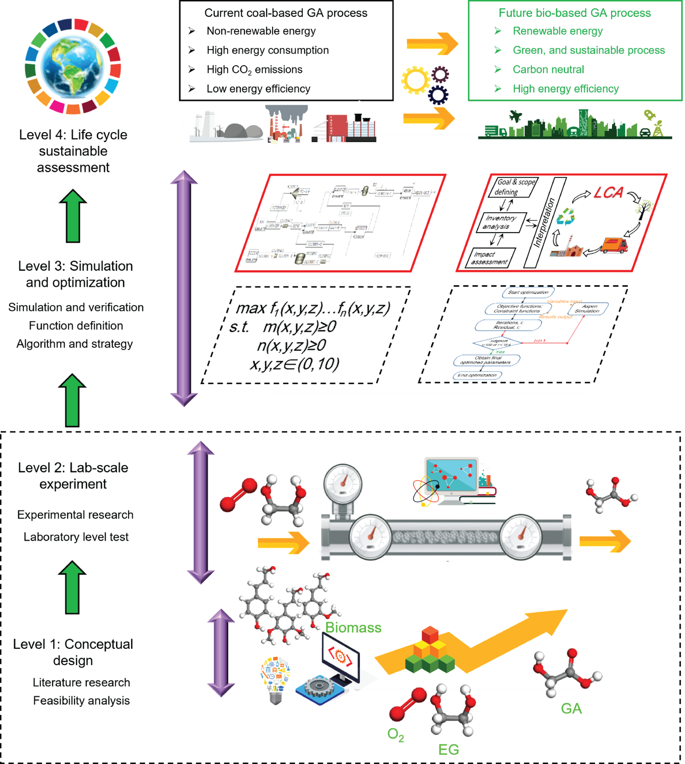
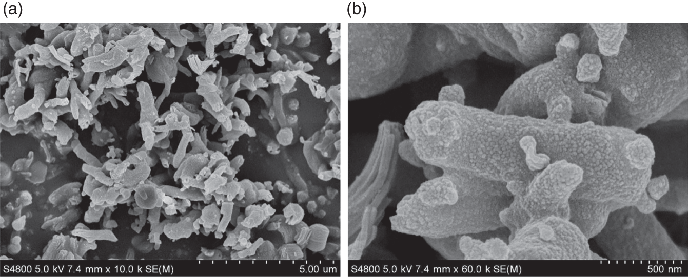
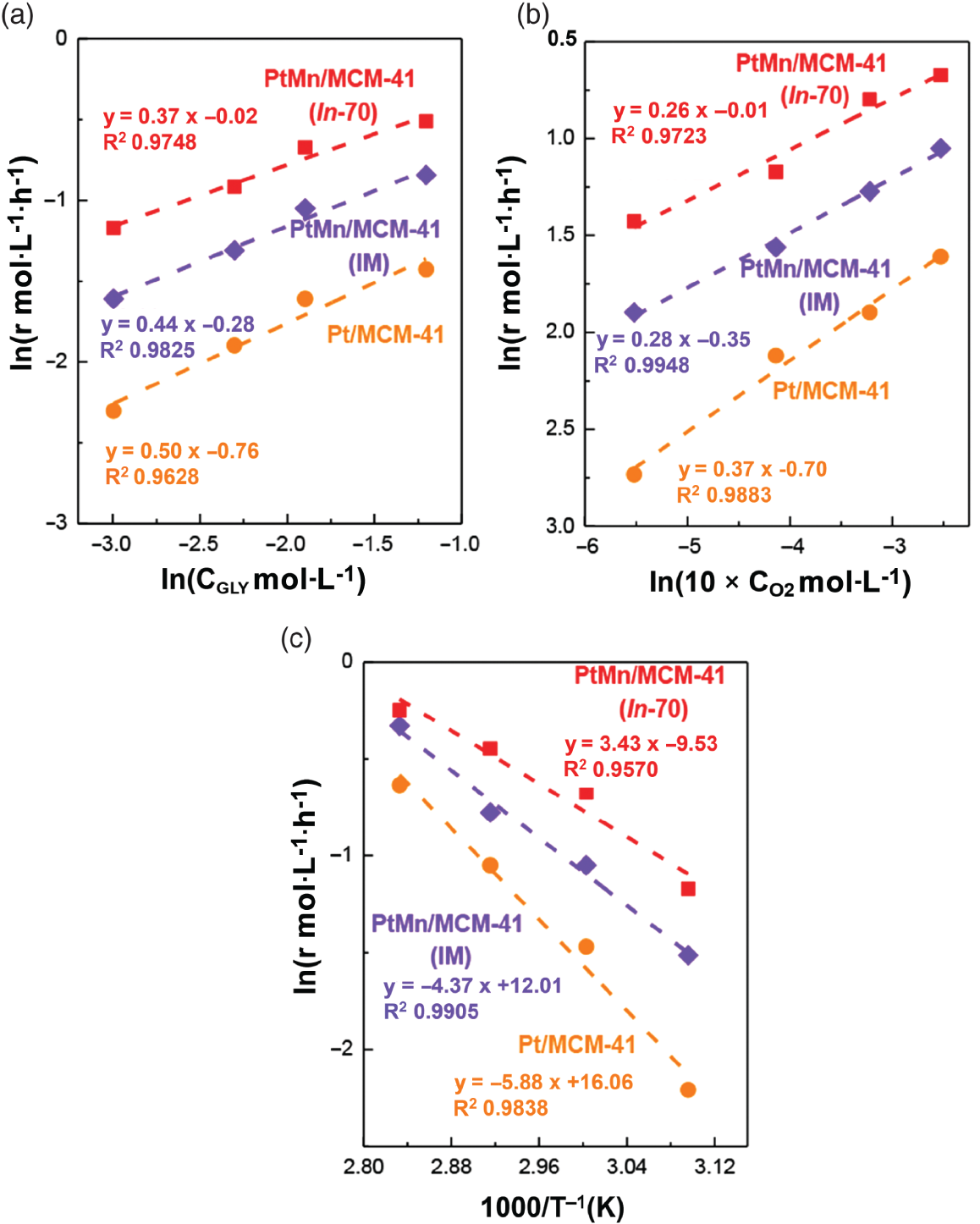
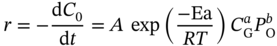
Xin Zhou Ocean University of China, College of Chemistry and Chemical Engineering, 238 Songling Road, Qingdao, Shandong 266100, China Dwindling fossil fuel resources [1], increasingly serious waste disposal problems [2], and the accumulation of nonbiodegradable plastic waste have become significant problems for the environment and sustainable ecosystems [3, 4]. To date, the world is estimated to have produced over eight billion tons of nondegradable plastic waste [5], of which only 9% was recycled and another 12% is incinerated [6]. The remaining 79% of trash accumulated in landfills or the natural environment is thrown out and deposited on refuse landfills or aquatic ecosystems [7]. The singularly inappropriate approach to plastic solid waste directly contributes to a surge in CO2 emissions [8, 9], which in turn contributes to global warming and brings a grievous threat to the environment and health of living things on the earth [10–12]. Worldwide, the development of degradable materials [13–15], has become the “hot spot” to deal with the ecological and environmental problems caused by nondegradable plastics [16, 17]. Poly glycolic acid (PGA) [18, 19], a synthetic polymer material with high-level biodegradability, makes it an ideal and versatile material for developing biodegradable and biomass-derived plastics to replace nondegradable plastics [20–22]. PGA also exhibits good biocompatibility and can be applied to human tissue and biomedical engineering, such as absorbable surgical sutures, biodegradable cardiovascular stents, and enhancing bone regeneration [23, 24]. The annual demand for PGA has increased rapidly [25]. The global bioresorbable polymers market size is estimated to be USD 417 million in 2022 and is projected to reach USD 688 million by 2027, at a compound annual growth rate (CAGR) of 10.5% between 2022 and 2027 [26]. Statistics show that the global demand for PGA Market is presumed to reach the market size of nearly USD 15.64 Billion by 2032 from USD 6.62 Billion in 2023 with a CAGR of 10.02% under the study period 2024–2032. [27]. However, faced with the above momentous application requirements, the production capacity of PGA is insufficient. One of the main reasons is the inadequate production capacity of PGA’s high-purity monomer GA [19]. The hydroxyl and carboxyl groups in the GA structure can be complex with other ions. This complex is difficult to remove. In addition, GA is easy to self-polymerize into low-molecular-weight glycolic acid dimer, glycolic acid tetramer, and other byproducts [28]. These characteristics of glycolic acid are difficult to purify, which will directly lead to the low purity of GA crystal [29]. If the purpose is to synthesize high-purity GA crystals, this will put forward high requirements for the synthesis and separation process of GA. The process technologies used for GA industrial synthesis and production mainly involve the hydrolysis of hydroxyacetonitrile [30], the hydrolysis of chloroacetic acid [19], the hydrolysis of methyl glycolate [31], and the carbonylation of formaldehyde [32]. Among these GA synthetic routes, developing a green process for synthesizing glycolic acid with fewer byproducts is crucial. Our previous research indicated a few byproducts from ethylene glycol as raw material through highly efficient Pt–Mn2O3 nanocatalysts, including only a tiny amount of glyoxylic acid and formic acid [33, 34]. Moreover, the industrial scale-up simulation and conceptual process design also show that the selective oxidation of ethylene glycol to GA (EGtGA) has superior techno-economic performance to conventional processing routes [35]. Therefore, the direct preparation of GA from ethylene glycol with a low market price has a promising industrial application prospect. It is the premise of producing high-purity GA to identify the essential factors affecting the target product GA, improve the yield of target product GA, and reduce the content of other byproducts [36, 37]. The operation parameters of the EGtGA process, such as reaction temperature and residence time, affect the GA yields, process energy consumption, and net present value [35]. Hence, it is feasible to improve the yield and quality of GA by adjusting these key factors. In addition, other related aspects in the EGtGA process, such as temperature, catalysts [38], and separation process [39], may also substantially impact GA’s yields and techno-economic performance. However, due to the high experimental costs and the time and energy cost of repeating experiments, it is a great challenge to study all the above factors and determine the optimal value of essential elements to manufacture GA with high purity. Due to the rapid rise of artificial intelligence [40], machine learning (ML) methods have gradually evolved into an effective strategy to address complex nonlinear issues (i.e. regression and classification with high order and multiloop) [41]. The ML approach has been employed to predict the yields of complex catalytic processes in the chemical engineering field [42, 43]. Using artificial intelligence to model and predict the properties and distribution of products in the chemical engineering reaction process can significantly save time and cost. The random forest (RF) ML model with high prediction accuracy was established to predict the mass yields and properties of specific products produced by the reaction of different raw materials under other conditions [44]. Compared with the RF model and support vector machine model, the prediction accuracy of the deep neural network (DNN) model is the highest, and the average R2 of the optimized DNN model is higher than 0.90. Thybaut and coworkers systematically compared the prediction results of ML methods in Fischer–Tropsch reaction models [45]. The results show that the deep belief network (DBN) model is superior to other verifying indicators [45, 46]. Furthermore, multiple linear regression, support vector machines, extreme gradient boosting (XGboost), and RF models have been employed to guide the optimization of product distribution and improve the yield of target products in the catalytic conversion process [47, 48]. Based on the above research background, selecting appropriate artificial intelligence modeling methods and developing ML prediction models with good accuracy will play an essential role in improving the yield of target products in the chemical process. Hence, many studies have been carried out to make up for the gap between the prediction of input variables, including raw material properties and operating conditions, and the yield and properties of output key target products [49, 50]. To improve the accuracy of artificial intelligence modeling, a large amount of data is usually needed for training. However, in the research and development stage of the chemical process, especially in the laboratory pilot stage, it is incredibly time-consuming and costly to obtain massive experimental data (such as thousands of sets of data) required for artificial intelligence modeling. Moreover, the progress of existing artificial intelligence model research in accelerating engineering and guiding the production of polymer-grade pure glycolic acid is still limited. In the previous work, the laboratory pilot stage, reaction kinetics solution, and conceptual process design of glycolic acid production were realized by selective oxidation with ethylene glycol as raw material and efficient Pt-based nanocatalysts [30]. Based on this, the ML prediction model of the yield and characteristics of polymerization grade glycolic acid “dual-core driven” by coupling data and reaction kinetics is successfully established in this study. The hybrid data and mechanism “dual-core driven” deep learning model, termed the HDM model, is developed to guide experimental research and optimize operating conditions. Concretely, data expansion is implemented to enrich the cube based on reaction kinetics to meet the challenge of data scarcity. In this study, more than 6000 mechanism-driven virtual data points are created and synthesized to enhance the model’s prediction ability, which is the main innovation of this paper. Then, the ML model is trained to predict the yield of the process products. The relative importance of each input to the target is further analyzed. The multi-objective optimization method based on the genetic algorithm is used to optimize the expected polymer-grade glycolic acid production process (maximize the yield, purity, and economic benefits of glycolic acid as well as minimize energy consumption). Finally, experiments and process simulation verify that the optimized operating conditions can produce polymeric glycolic acid with low energy consumption, high purity, high yield, and high economic performance. The framework for predicting GA production performance includes five steps, as illustrated in Figure 4.1. Through the case study of the EGtGA process, the detailed implementation of our framework is further introduced. Step 1: Database generation. The feature variables were first determined. Based on the existing experimental data, a representative reaction kinetic model, including the EGtGA process, was established and simulated to generate the yield dataset of key products for steady-state simulation. The correlation between features and targets was further analyzed. Figure 4.1 The overall research framework for predicting glycolic acid production by selective oxidation of ethylene glycol using deep learning. Source: Zhou et al. [51]/with permission from John Wiley & Sons. Step 2: Data preprocessing. Developing the detailed database and introductory programming (i.e. loading ML library functions and reading database files). Step 3: Deep learning. Building ML or deep learning models and performing model training, testing, and prediction. Step 4: Comparative analysis. The performance and robustness of various ML models, namely deep neural networks, DBNs, fully connected residual network (FC-ResNet), and RF regression, were compared to identify the most appropriate ML model for the EGtGA process. Step 5: Optimization and prediction. Predict the yields and performance of critical products in the EGtGA process to verify the trained FC-ResNet model. The optimal operating parameters for the highest yield of GA were obtained and verified by experiments. The genetic algorithms were used to optimize the model parameters (such as iterations) of the ML model, and the optimized parameters were used to train the ML model. Step 6: Multidimensional evaluation. The EGtGA process was deeply analyzed and multi-dimensionally evaluated using optimal operating parameters based on the life cycle, economic, and social environment framework. The database used to train the ML model consists of many schemes with different characteristics and corresponding production performance. The first step of building the database is to select representative parameters as training features among the factors affecting GA production. We decided on 10 features that play an essential role in GA production as features (see Table 4.1). The EGtGA process model was established based on the conceptual design flow chart (see Figure 4.2a). A total of 610 sets of experimental datasets using different reaction conditions and catalysts were collected. Because of the advantages of steady-state simulation and process control, Aspen Plus has been widely used in process simulation, optimization, and prediction. Hence, the general process simulation software Aspen Plus was also applied to establish the simulation model of the EGtGA process. The process simulation consists of 13 process unit modules: compressor, continuous stirred tank reactor, vacuum column, and vacuum dividing wall column, as shown in Figure 4.2b. The binary interaction parameters of stream material compositions using the non-random two liquid (NRTL) method are adopted to calculate the phase equilibrium. The reaction kinetics and process models were established based on these experimental data. By using the process model developed by Aspen Plus, abundant process simulation data can be obtained. As a result, Aspen Plus process simulation software is applied to generate the data of 6110 cases through process simulation, fill the ML models, and enhance the database. It is worth noting that the hold-out method is used to achieve the dataset partitioning [51]. A small part is taken as the test set and verification set, and the rest is taken as the training set. The dataset partitioning details are shown as follows, training set:verification set:test set = 80% : 10% : 10%. The correlation performance was identified by analyzing the relationship between essential process operating parameters (reaction temperature, reaction residence time, and reaction pressure) and conversion and GA yield. The reaction networks of the EGtGA process and reaction activation energies (Pt loading 1.4 wt%; Mn loading 0.9 wt%) are demonstrated in Figure 4.2c. Table 4.1 The selected features and desired targets for deep learning. Figure 4.2 (a) conceptual design process flow chart; (b) simulation flowsheet in Aspen Plus; (c) reaction network and kinetics parameters (Pt loading 1.4 wt%; Mn loading 0.9 wt%). The computing environment conditions in this study are CPU: Intel (R) Core (TM) i7-10,700 CPU@2.90GHZ and GPU: NVIDIA GTX 1060. Therefore, a total of 5040 complete datasets, including experimental and simulation data, composed of process data, reaction kinetic parameters, and product yields, constitute a comprehensive database required for ML training. This work’s ML models mainly include DNN and RF. The neural network models considered in this work include a deep neural network, a DBN, and a FC-ResNet. The integrated algorithm, RF, is illustrated in the following part. The DNN is the feedforward neural network with multilayers [46]. It is one of the simplest neural network forms and has good prediction performance. These networks usually have three layers: the input layer, hidden layer, and output layer, as illustrated in Figure 4.3a. A gradient descent optimization method called backpropagation identifies or trains weights in neural networks. This procedure is represented visually in Figure 4.3b. In the feedforward neural network, the input layer has the same number of nodes as the input, and the input is directed to the subsequent layer. One or more hidden layers calculate the weighted sum of all outputs from the previous layer and regularize the weighted sum using the activation function. Activation functions include linear, sigmoid, hyperbolic tangent, exponential linear unit, rectified linear unit, and scaled exponential linear unit. The output layer repeats the same process as the hidden layer with its unique weight. Each weight in the system will be updated in each training process, and the updated amount is determined by distinguishing the prediction error from their respective weights. Using the differential chain rule, the backpropagation algorithm is computationally efficient because almost all components of each derivative are calculated during the forward transmission (i.e. prediction calculation) of the network and can be reused when updating the weight. Figure 4.3 (a) Neural network structure of each layer node in DNN; (b) backpropagation calculation algorithm. The DBN is a probability generation model for unsupervised and supervised learning [52]. Compared with the traditional neural network, the generation model establishes a joint distribution between observation data and labels. DBN comprises multilayer neurons divided into dominant and recessive neurons. The bottom layer represents data vectors, and each neuron represents one dimension of the data vector. The component of DBN is restricted Boltzmann machines (RBMs). The DBN model can extract features layer by layer from the original data and obtain high-level representations through the layer-by-layer stacking of RBMs. Its core is to use the layer-by-layer greedy learning algorithm to optimize the connection weight of the deep neural network, that is, first use the unsupervised layer-by-layer training method to effectively mine the fault characteristics of the equipment to be diagnosed, and then, based on adding the corresponding classifier, optimize the fault diagnosis capability of the DBN through the reverse supervised tuning. The unsupervised layer-by-layer training can learn complex nonlinear functions by directly mapping data from input to output, which is also the key to its robust feature extraction ability. The training goal of RBM is to make the Gibbs distribution fit the input data as much as possible, that is, to make the Gibbs distribution represented by the RBM network as close as possible to the distribution of input samples. The Kullback–Leibler (KL) distance between the sample distribution and the edge distribution of the RBM network can be used to express the difference between them. Because the deep network quickly falls into local optimization, and the selection of initial parameters significantly impacts where the network finally converges, DBN training is divided into pretraining and fine-tuning. RBM performs layer-by-layer unsupervised training on the deep network and takes the parameters obtained from each layer of training as the initial parameters of neurons in each layer of the deep network. This parameter is in a good position in the deep network parameter space, pretraining. After RBM trains the initial values of the deep network parameters layer by layer, it trains the deep network with the traditional backpropagation (BP) algorithm. In this way, the parameters of the deep network eventually converge to a good position, that is, fine-tuning. In the pretraining, the unsupervised layer-by-layer learning method is used to learn the parameters. First, the data vector x and the first hidden layer are used as an RBM to train the RBM parameter. Then, the RBM parameter is fixed, h1 is used as the visible layer vector, h2 is used as the hidden layer vector, and the second RBM is trained. The whole neural network can generate training data according to the maximum probability by training the weights between its neurons. DBN can be used not only to identify features and classify data but also to generate data. DBN comprises multilayer neurons divided into dominant and recessive neurons. The graphic element accepts input and the implicit part extracts features. Therefore, hidden elements also have an alias called feature detectors. The connection between the top two layers is undirected and forms associative memory. There are connections between other lower layers and directed connections up and down. The bottom layer represents data vectors, and each neuron represents one dimension of the data vector. RBM and its training process are shown in Figure 4.4a. The method of training DBN is carried out layer-by-layer. The hidden layer of the previous RBM provides input to the next visible layer. Figure 4.4b illustrates a schematic diagram of a DBN composed of three RBM layers. In each layer, the data vector is used to infer the hidden layer, and then the hidden layer is regarded as the data vector of the next layer. Each RBM can be used as a separate cluster. RBM has only two layers of neurons. One layer is called the visible layer, composed of visible units used to input training data. The other layer is called the hidden layer. Accordingly, it is composed of hidden units used as feature detectors. The visible layer of the lowest RBM receives the input characteristic data, and the hidden layer of the highest RBM is connected to the backpropagation layer to obtain the model output. Figure 4.4 (a) Network structure and training process of restricted Boltzmann machine; (b) the structure of DBN composed of three-layer RBM. The model accuracy is continuously improved with the continuous increase in network layers. However, the network reaches saturation when the network layers increase to a certain number. Training and testing accuracy will decline rapidly, indicating that the deep network with more layers is challenging to train. The deeper the network layers are, the worse the prediction effect is because the neural network will continuously propagate the gradient in the backpropagation process. When the network layers are more profound, the gradient will gradually disappear in the propagation process (if the sigmoid function is used, for the signal with an amplitude of 1, the gradient will decay to the original 0.25 every time it is transmitted back, and the more layers, the more severe the attenuation). As a result, the weight of the previous network layer cannot be effectively adjusted. He et al. proposed the residual network (ResNet) [53]. The ResNet model can continue improving the network’s training and test accuracy when the original network is close to saturation. Adding ResNet structure to the network can solve the problematic network convergence caused by deepening the network layers and helping the whole network converge faster. Figure 4.5a shows a 4-layer fully connected network with 14 nodes in the input layer and 5 nodes in the output layer. The general network structure is shown in Figure 4.5b, and the ResNet structure is shown in Figure 4.5c. When the ResNet is constructed in the form of a full connection, it constitutes a FC-ResNet. It is difficult to directly let some layers fit a potential identity mapping function (see Eq. (4.1)), which may be why it is challenging to train the deep neural network. However, if the network is designed as Eq. (4.2), we can transform it into learning a residual function, as defined in Eq. (4.3). When F(x) equals zero, it constitutes an identity map. If the residual is not zero, the accumulation layer learns new features based on the input features to perform better. Figure 4.5 (a) 4-Layer fully connected network with 14 nodes in the input layer and 5 nodes in the output layer; (b) structure unit of general network structure; (c) structure unit of ResNet unit. Suppose an existing shallow network (Shallow Net) has reached saturation accuracy. Then several identity mapping layers (y = x, output equals input) are added to it so that the depth of the network is increased. At least the error will not increase. That is, the deeper network should not increase the error on the training set. The inspiration of the deep ResNet is to use identity mapping to directly transmit the previous layer’s output to the rear mentioned here. RF is composed of multiple decision trees [54]. Each decision tree is different. When building the decision tree, we randomly select some samples from the training data, and we will not use all the features of the data but randomly select some features for training. Each tree uses different samples and features, and the training results are also different. RF applies the general technique of bootstrap aggregating to tree learners. As depicted in Figure 4.6, assuming that the training data includes B inputs (X = X1, …, XB) and responses (y = y1, …, yB), bagging could select a random sample back and forth. It replaces the training data B times to train the tree fB on XB, and Yb (b = 1, …, b). When constructing the regression tree, m features or input variables are randomly selected from P features or input variables (m < P), called feature bagging. Each regression tree grows freely without restriction until it cannot continue to split. That is, it reaches the minimum node size. Finally, B regression trees form the RF algorithm. The advantage of RF is quite outstanding. It has the following benefits: (i) using an integrated algorithm with high accuracy, (ii) not easy to have overfitting (random samples and random characteristics), (iii) strong anti-noise ability (noise refers to abnormal data), and (iv) processing high-dimensional data with many features. Figure 4.6 Flowsheet of random forest method. A genetic algorithm is based on natural selection and genetics [55, 56]. Since the 1990s, it has been widely used because of its high efficiency and strong robustness. In the genetic algorithm, the candidate solution group of an optimization problem evolves toward a better solution. Evolution starts with a group of randomly generated individuals, an iterative process. The population in each iteration is called a generation. In each generation, the adaptability of each individual in the population is evaluated. More suitable individuals are randomly selected from the current population, and each individual’s genome is modified (recombined, possibly random mutation), forming a new generation. The next-generation candidate solutions are then used in the next iteration. Usually, when the generated algebra reaches the maximum population’s satisfactory fitness level, the algorithm terminates. In this study, the genetic algorithm and HDM models are combined to optimize the model parameters of the four deep learning models. It effectively searches the minimum objective function and avoids the calculation and analysis of each response. This paper uses the high-performance and practical Python genetic algorithm toolbox to optimize. Although recent advances in life cycle methodology have expanded the range of environmental impacts considered, including biodiversity and ecosystem services [57], when considering social and livelihood factors, the application trend of life cycle assessment in these critical aspects is still limited. Life cycle sustainability assessment (LCSA) can assess the impact of target products, processes, and supply chain decisions on the ecological environment for projects from multiple dimensions [58]. In this study, LCSA can quantitatively provide a feasible framework for the proposed dual-core-driven process model. To analyze the impact of the proposed HDM model on society, people’s livelihood, and the environment, the multidimensional sustainability assessment method of the life cycle proposed in our previous work is adopted. In this method, greenhouse gas (GHG) emissions and fossil energy demand (FED) are integrated into the comparison range of gross domestic product (GDP, US$) generated based on the HDM model [59, 60]. Figure 4.7 depicts the detailed data (including feature categories and ranges) with a residence time of eight hours in the experimental dataset. Other experimental data with residence times of 4–12 hours are depicted in Appendix. The X-axis and Y-axis of the three-dimensional image are reaction temperature and pressure, respectively. According to the composition analysis of chromatographic data, the reaction temperature is the main characteristic factor affecting the conversion and other key indicators. The conversion rate fluctuates in a wide range, ranging from 0% to 100%. The two basic characteristic categories are residence time and reaction pressure, the other two key indicators to determine the product distribution in the EGtGA process. GA yields, glyoxalic acid (GAD) yields, formic acid (FA) yields, and CO2 yields range from zero to the upper limit of 9–89%. The above results show that this study’s preliminary experimental dataset is 610 groups. The experimental data is extensive enough to cover a broader range of product distributions and support constructing a mechanism model. The database of the “dual-core-driven” deep learning HDM model also includes parameters such as reaction rate constants and activation energy. The reaction temperature of the HDM model was 20–90 °C, the reaction pressure was 1–3 MPa, and the residence time was 4–12 hours. By comprehensively analyzing Figure 4.7 and the database, we can intuitively conclude that the reaction temperature is the most crucial factor affecting the product yield of the EGtGA process. In terms of the yield of the target product, the GA yield is between 0.73% and 75.85%. The yield of CO2 and formic acid from the EGtGA process is between 0.11% and 54.11% and 0.01–9.43%. Due to the different reaction conditions of the HDM model, the product yield distribution has a large span. This also strengthens our determination to perform the HDM model to identify further and tune essential factors affecting the EGtGA process to produce the highest yield of glycolic acid product. Figure 4.8 illustrates the heat map of the linear regression correlation coefficient matrix between the selected features and the desired targets. The deep blue and light navy blue grids (absolute value ≥0.80) show strongly positive and negative correlations, respectively. It can be seen that some areas on both sides of the diagonal of the grid are relatively deep, indicating that there is a linear relationship between the conversion and immediate product yield of the EGtGA process and these features. For example, the conversion rates of the HDM model represent strongly positive correlations with reaction temperature (see F1 in Table 4.1), in which the correlation coefficient value is 0.913. Figure 4.7 Data analysis and statistics with the reaction condition resident time eight hours: (a) the changing trend of conversion rates with reaction temperature and pressure; (b) the changing trend of GA yields with reaction temperature and pressure; (c) the changing trend of GAD yields with reaction temperature and pressure; (d) the changing trend of FA yields with reaction temperature and pressure; (e) the changing trend of CO2 yields with reaction temperature and pressure. Further analysis is carried out based on the above four HDM models to provide more details about each target’s prediction performance and input characteristics’ role. Figures 4.9–4.13 show each target’s predicted and actual values. The setting of model parameters greatly influences the prediction results of R2 and root-mean-square error (RMSE) in the ML model. Unreasonable learning rates and iteration times are straightforward to produce overfitting. Therefore, DNN, DBN, and FC-ResNet have the same number of neural network iterations, 500, and the neural network learning rate is 0.0001 in this study. In the RF method, the max_depth and n_estimators are 10 and 100, respectively. The experiment and prediction values of convention rates (training and testing) in the HDM model by DNN, DBN, FC-ResNet, and RF are shown in Figure 4.9a–d. The conversion prediction result of the EGtGA process is in the range of 20–97%. It is worth noting that the R2 of the “dual-core driven” HDM model for the conversion prediction is 0.932–0.996. Moreover, a comprehensive comparison of Figure 4.9 shows that the R2 of the FC-ResNet method is the highest at 0.996, which is also the lowest of its RMSE of 1.37. Figure 4.8 Heat map of the linear regression correlation coefficient matrix between the selected features and the desired targets. The experiment and prediction values of GA yields in the EGtGA process (training and testing) in the HDM model by DNN, DBN, FC-ResNet, and RF are shown in Figure 4.10a–d. The GA yield prediction results of the EGtGA process are in the range of 0.02–79.5%. It is worth noting that the R2 of the “dual-core driven” HDM model for the conversion prediction is 0.902–0.988. Similarly, a comprehensive comparison of Figure 4.10 shows that the R2 of the FC-ResNet method is the highest at 0.988, which is also the lowest of its RMSE of 1.95. Figure 4.9 Experiment and prediction values of EGtGA convention rates (training and testing) in the HDM model based on (a) DNN, (b) DBN, and (c) FC-ResNet, (d) RF. Figure 4.11 depicts the experiment and prediction values of GAD yields in the EGtGA process (training and testing) in the HDM model by DNN, DBN, FC-ResNet, and RF. The absolute value of GAD yield prediction results of the EGtGA process is in the range of 0.02–9.21%. It is worth noting that the R2 of the “dual-core driven” HDM model for the prediction is 0.913–0.996. Similarly, a comprehensive comparison shows that the R2 of the FC-ResNet method is the highest at 0.996, which is also the lowest of its RMSE of 0.17. Figure 4.12 illustrates the experiment and prediction values of FA yields in the EGtGA process (training and testing) in the HDM model by DNN, DBN, FC-ResNet, and RF. A comprehensive analysis shows that the prediction results of DNN and DBN are worse than those of FC-ResNet and RF. The absolute value of FA yield prediction results of the EGtGA process is in the range of 0.24–19.13%. It is worth noting that the R2 of the “dual-core driven” HDM model for the conversion prediction is 0.899–0.995. Similarly, a comprehensive comparison depicts that the R2 of the FC-ResNet method is the highest at 0.995, which is also the lowest of its RMSE of 0.35. Figure 4.10 Experiment and prediction values of GA yields in the EGtGA process (training and testing) using the HDM model based on (a) DNN, (b) DBN, and (c) FC-ResNet, (d) RF. The experiment and prediction values of FA yields in the EGtGA process (training and testing) in the HDM model by DNN, DBN, FC-ResNet, and RF are demonstrated in Figure 4.13. Similar to Figure 4.12, it can be seen visually that the DNN and DBN prediction results are also worse than those of FC-ResNet and RF. The absolute value of CO2 yield prediction results of the EGtGA process is 0.12–77.29%. It is worth noting that the R2 of the “dual-core driven” HDM model for the conversion prediction is 0.960–0.998. A comprehensive comparison shows that the R2 of the FC-ResNet method is the highest at 0.998, which is also the lowest of its RMSE of 0.84. Figure 4.11 Experiment and prediction values of GAD yields in the EGtGA process (training and testing) using the HDM model based on (a) DNN, (b) DBN, and (c) FC-ResNet, (d) RF. This study further adopts the “dual-core driven” models to perform the prediction and provides the calculation results of feature importance. There are apparent differences between the method of calculating feature weight by the deep neural networks and the method of calculating RF. The idea of the neural network to estimate the importance of features is based on a permutation algorithm. The core idea of this algorithm is to train a neural network first. When calculating the importance of the ith feature, disrupt the ith feature, and then calculate the index change after the disruption. The importance calculation method of the corresponding features of RF is: if the accuracy outside the bag decreases significantly after adding noise to a feature randomly, it shows that this feature has a significant impact on the classification results of samples, that is, its importance is relatively high. Figure 4.12 Experiment and prediction values of FA yields in the EGtGA process (training and testing) using the HDM model based on (a) DNN, (b) DBN, and (c) FC-ResNet, (d) RF. Figure 4.14 depicts each input feature’s importance to the HDM model’s five targets. It can be found that there is a certain difference between the results of calculating the importance of characteristics in the neural network like dual-core driven model and RF. Figure 4.14a–c intuitively shows that reaction activation energy and catalyst features (including Pt loading, Mn loading, and TOF) are more critical than reaction conditions. The sum of specific feature importances (reaction activation energy, catalyst composition, and TOF) is 70–71%, which are the dominant and decisive factors. Furthermore, the results of all feature importances show that the activation energy of the second step reaction (see Figure 4.2c) is the most important feature. This also confirms our previous research results. The second step reaction is the rate control step in the process of ethylene glycol oxidation to glycolic acid. Figure 4.13 Experiment and prediction values of CO2 yields in the EGtGA process (training and testing) using the HDM model based on (a) DNN, (b) DBN, and (c) FC-ResNet, (d) RF. From Figure 4.14, it can be found that the reaction temperature is the dominant factor. The differences between the two kinds of algorithms cause the above differences. Similarly, the sum of specific feature importance (reaction activation energy, catalyst composition, and TOF) is about 65% in Figure 4.14d, which are also the dominant factors. They all clearly showed that the reaction activation energy, catalyst composition, and TOF were the main features affecting the conversion and yield of the EGtGA reaction. Since our study is committed to providing a “dual-core drive” model that can predict and optimize the industrial application of the EGtGA process in the future, we have chosen features that are biased toward the macro in the subsequent optimization process. Hence, catalyst compositions (Pt loading and Mn loading) and reaction conditions (reaction temperature, reaction time, and reaction pressure) were selected as decision variables of the multi-objective optimization. Figure 4.14 Results of feature importances for: (a) DNN, (b) DBN, (c) FC-ResNet, and (d) RF. By comprehensively analyzing four deep learning algorithms (DNN, DBN, FC-ResNet, and RF), it can be intuitively concluded that compared with the other three methods, FC-ResNet performs very well in both the training set and the test set. For the training set, the RMSE of the FC-ResNet algorithm for predicting conversion rate, GA yield, GAD yield, FA yield, and CO2 yield are 1.55, 1.18, 0.15, 0.25, and 0.17, respectively. For the test set, the RMSE of the FC-ResNet algorithm for prediction conversion, GA yield, GAD yield, FA yield, and CO2 yield are 1.37, 1.95, 0.17, 0.25, and 0.17, respectively. For the experimental data, the RMSE of the FC-ResNet algorithm for both the training set and test set is the lowest, showing excellent prediction performance. Therefore, the model parameters of FC-ResNet, by integrating the GA, were optimized in this section. Moreover, the optimized FC-ResNet algorithm (termed FC-ResNet–GA) will also be applied to train and test 6720 datasets (including 610 mechanism datasets and 6110 experimental datasets). Figure 4.15 shows the training and test results for the simulation and experiment data in the EGtGA process using the HDM model based on the FC-ResNet–GA model. As illustrated in this figure, the RMSE of the FC-ResNet–GA model for the training set to predict conversion rate, GA yield, GAD yield, FA yield, and CO2 yield are 1.53, 1.93, 0.03, 0.05, and 0.86, respectively. For the test set, the RMSE of the FC-ResNet algorithm for prediction conversion, GA yield, GAD yield, FA yield, and CO2 yield are 1.12, 1.29, 0.06, 0.07, and 0.56, respectively. Further investigation is carried out, and multi-objective optimization of process parameters is implemented using the HDM model based on the FC-ResNet–NSGA-III model. In this section, this study uses Python 3.8 to program and apply the NSGA-III algorithm in Pymoo to perform multi-objective optimization of process parameters and then solve the problem. Finally, the Pareto solution set that meets the requirements is obtained. The objective functions and constraints are shown in Eq. (4.4). The results of Pareto sets (mainly including reaction conditions and supported catalyst composition for experimental verification, such as reaction temperature, reaction pressure, reaction time, Pt loading, and Mn loading) for the process multi-objective optimization using the NSGA-III algorithm and experiment verification are illustrated in Figure 4.16. It should be pointed out that the results of Pt and Mn loading in the Pareto sets are 1.40 and 0.90, respectively. The experimental verification of repeatability is performed by adopting the feasible solution in the Pareto solution set. The relative errors between experiment and simulation repeatability verification of EG conversion and GA yield are about 4%, while the relative errors between experiment and simulation repeatability verification of GAD yield, CO2 yield, and FA yield are about 10%. The main reason is that GAD yields, CO2 yields, and FA yields are all in the range of low values (0–2%), and a small absolute error could bring about relatively significant errors. More detailed results of Pareto sets and experiment verification are shown in Appendix. Figure 4.15 The train and test results for the simulation + experiment data in the EGtGA process using the HDM model based on the FC-ResNet-GA model: (a) conversion, (b) GA yields, and (c) GAD yields, (d) FA yields, (e) CO2 yields, and (f) importance analysis. Figure 4.16 (a) The results of Pareto sets for the process multi-objective optimization using the NSGA-III algorithm and (b) experiment verification. Further LCSA investigation is implemented based on the optimized parameters. The original framework to execute the life cycle assessment is shown in Figure 4.17 [61, 62]. It should be mentioned that the black dashed box indicates the existing foundation, while the red implementation box indicates that the execution starts from the current step. As demonstrated, one of the feasible solutions applied in this study is reaction temperature, reaction pressure, reaction time, Pt loading, and Mn loading from the Pareto-optimal set, which are 63.53 °C, 1.54 MPa, 9.81 hours, 1.40 wt%, and 0.90 wt%, respectively. The selected feasible solution from the Pareto-optimal set is used to carry out the process simulation. Detailed and comprehensive life cycle inventory analysis is a crucial procedure for implementing LCSA, which can intuitively give critical data such as nonrenewable resources and energy consumption in different life cycle stages. These inventory data will lay a solid foundation for implementing sustainable life cycle interpretation and evaluation. Figure 4.18 demonstrates the life cycle assessment results of inventory values, which contain FED and GHG emissions in the form of direct and indirect for creating the one million GDP. Figure 4.18a shows the life cycle inventory analysis before optimization for the ethylene glycol (EG) to GA process using biomass as feedstock. The simulation data and inventory data are from our previous work [33, 34]. The simulation and inventory data of life cycle inventory analysis after optimization are depicted in Figure 4.18b. By comprehensively comparing the data before and after optimization, it can be intuitively concluded that the use of biomass raw materials has been reduced by about 3% by using the optimization strategy proposed in this study. Figure 4.17 The framework of life cycle multi-objective sustainable optimization. The black dashed box indicates the existing foundation, while the red implementation box indicates that the execution starts from the current step. Figure 4.19 illustrates the life cycle sustainable interpretation and evaluation results based on the inventory analysis from Figure 4.18. After optimization, the EG to GA process identifies obvious techno-economic and environmental advantages. As shown in Figure 4.19a, the FED after optimization is 6201.91 MJ (one million GDP)−1, which has decreased by 2.96%. The GHG emissions before optimization are 39.26 tCO2eq (one million GDP)−1, 1.03 times larger than the emissions after optimization (see Figure 4.19b). The breakdown analysis of FED and GHG is illustrated in Figure 4.19c,d. The decomposition results of each unit’s life cycle sustainability analysis are carried out to recognize further the bottleneck units hidden in the EGtGA process. The syngas production process contributes the most to FED and GHG emissions, accounting for about 68% of the whole FED and 45% of the whole GHG, respectively. The sustainability analysis results intuitively indicate that syngas production is the most extensive bottleneck process. Therefore, optimizing parameters in the syngas production process and developing energy recovery technology is virtual to enhance the process performance. Figure 4.18 The life cycle inventory analysis for the EG to GA process using biomass as feedstock: (a) before optimization; (b) after optimization. Figure 4.19 Overall resource consumption, greenhouse gas emission results, and the breakdown distribution analysis of FED and GHG for the EG to GA process: (a) Overall results of FED; (b) Overall results of GHG; (c) breakdown results of FED; (d) breakdown results of GHG. The kinetic reaction mechanism, catalyst properties, and reaction conditions in the cases of selective oxidation at low temperatures without alkali for bio-GA production were collected to construct a hybrid deep learning framework driven by data and reaction mechanisms for predicting sustainable glycolic acid production performance. The FC-ResNet model exhibited superior performance for the prediction of conversion rate, GA, and byproduct yields. The feature importance was further analyzed. Reaction activation energy and other features (Pt loading, Mn loading, and TOF) are far less critical than reaction conditions and rates. The reaction conditions are the dominant and decisive factor, the influence of the reaction rate is low, and other characteristics are far less critical than reaction conditions. The HDM model based on the FC-ResNet–NSGA-III model is implemented with multi-objective optimization of process parameters. The results of Pareto sets were obtained, and the optimized models were experimentally validated. The selected parameters, including reaction temperature, reaction pressure, reaction time, Pt loading, and Mn loading from the Pareto-optimal set are 63.53 °C, 1.54 MPa, 9.81 hours, 1.40 wt%, and 0.90 wt%, respectively. Detailed and comprehensive life cycle inventory analysis was also implemented. The LCSA further identifies that using the optimized operating parameters, the FED, and GHG have decreased by 2.96% and 3.00%, respectively. The hybrid data and mechanism (HDM) model offers a novel insight and strategy to accelerate the engineered selective oxidation for desired GA production. Pareto-optimal solution is a multi-objective intelligent algorithm. Pareto-optimal solution is a multi-objective solution that will filter out a relatively optimal set of solutions. Pareto will be used to find a reasonably optimal solution or optimal solution. In this study, the Pareto-optimal solution set is shown in Figure 4.A.1. The Pareto-optimal solution set only provides noninferior solutions of the problem to multiple objectives. In this study, the reaction conditions in the red box are selected as the optimal solution. Figure 4.A.1 The Pareto optimization Set. Data for reaction residence times of 4–12 hours was established and shown in Figure 4.B.1 and 4.B.2. Figure 4.B.1 Data analysis and statistics with the reaction condition resident time four hours: (a) the changing trend of conversion rates with reaction temperature and pressure; (b) the changing trend of GA yields with reaction temperature and pressure; (c) the changing trend of GAD yields with reaction temperature and pressure; (d) the changing trend of FA yields with reaction temperature and pressure; (e) the changing trend of CO2 yields with reaction temperature and pressure. Figure 4.B.2 Data analysis and statistics with the reaction condition resident time 12 hours: (a) the changing trend of conversion rates with reaction temperature and pressure; (b) the changing trend of GA yields with reaction temperature and pressure; (c) the changing trend of GAD yields with reaction temperature and pressure; (d) the changing trend of FA yields with reaction temperature and pressure; (e) the changing trend of CO2 yields with reaction temperature and pressure. On the basis of the above reaction mechanism identification, we analyzed the possible reaction path of the Pt catalyst used in the selective oxidation of ethylene glycol to glycolic acid. The reaction path diagram is shown in Figure 4.C.1. Based on the reaction path shown in Figure 4.C.1, the reaction kinetics parameters in this study are obtained by regression based on the reaction mechanism and a large number of experimental data. The detailed steps of the calculation process of the reaction kinetics parameters we performed are shown below. The detailed description is shown as follows (the description and Figure 4.C.2): Figure 4.C.1 The reaction networks in the EGtGA process. Figure 4.C.2 The detailed flowsheet of the database generation procedure. The following further elaborates on the reaction kinetics regression steps used in this chapter. In this part, we will use the PtMn/MCM-41 (Pt loading 1.4 wt%; Mn loading 0.9 wt%; termed as In-70) catalyst as the example. More detailed information is also shown in our previous work (Applied Catalysis B: Environmental 2021, 284, 119803). The PtMn/MCM-41 (Pt loading 1.4 wt%; Mn loading 0.9 wt%) was selected to study the internal and external mass transfer. It is ensured that all the catalysts were evaluated with negligible mass transfer limitations. (Reaction conditions: 60 °C, 1 MPa O2, 0.15 M EG, 0.1 g Cat.) Figure 4.C.3 SEM images of MCM-41. The reaction order for the EG concentration (CG) (a) of the Pt/MCM-41, PtMn/MCM-41 (IM) and PtMn/MCM-41 (In-70) catalysts are 0.50, 0.44 and 0.38, respectively. This suggests that the PtMn catalysts have stronger adsorption ability for EG than monometallic Pt/MCM-41 catalyst, and the Pt-Mn2O3 interfacial active site in the PtMn/MCM-41 (In-70) catalyst further promotes the adsorption of EG, which is well consistent with the DFT calculation results. Meanwhile, the PtMn/MCM-41 (In-70) catalyst displays the minimum reaction order for O2 pressure (PO) (b) (0.26) compared with the other two catalysts, meaning that the PtMn/MCM-41 (In-70) catalyst strongly adsorbs oxygen, probably due to the relatively faster replenishment rate of the consumed surface molecular oxygen [33]/with permission of Elsevier. As shown in Figure 4.C.4, the power function type reaction kinetic equation was employed to investigate the reaction orders for EG and O2 over the PtMn/MCM-41 (Pt loading 1.4 wt%; Mn loading 0.9 wt%, termed as In-70) and Pt/MCM-41 catalysts (Pt loading 1.3 wt%). The equation can be expressed as: Figure 4.C.4 The effects of (a) EG concentration and (b) oxygen pressure on the oxidation of EG. Reaction conditions: 25 ml of EG aqueous solution (0.15 M), 0.1 g Cat., T = 60 °C, stirring speed = 1000 rpm. (c) Apparent activation energy for EG conversion. CEG and PO are the initial concentration of ethylene glycol and O2 pressure (mol l−1) respectively; a and b are the corresponding reaction order. r, T, A, R, and Ea are the initial reaction rate of glycerol (in mol l−1 h−1), reaction temperature (K), the pre-exponential factor, ideal gas constant (8.314 × 10⁻³ kJ mol−1 K−1), and activation energy (kJ mol−1). It should be noted that the concentration of oxygen at the surface equals its bulk concentration (calculated by Henry’s law) under the reaction conditions (J. Phys. Chem. C 2010, 114, 1164–1172; J. Chem. Thermodyn. 2000, 32, 1145; J. Phys. Chem. 1996, 100, 5597).
4
Integration of Observed Data and Reaction Mechanisms in Deep Learning for Designing Sustainable Glycolic Acid
4.1 Introduction
4.2 Methodology

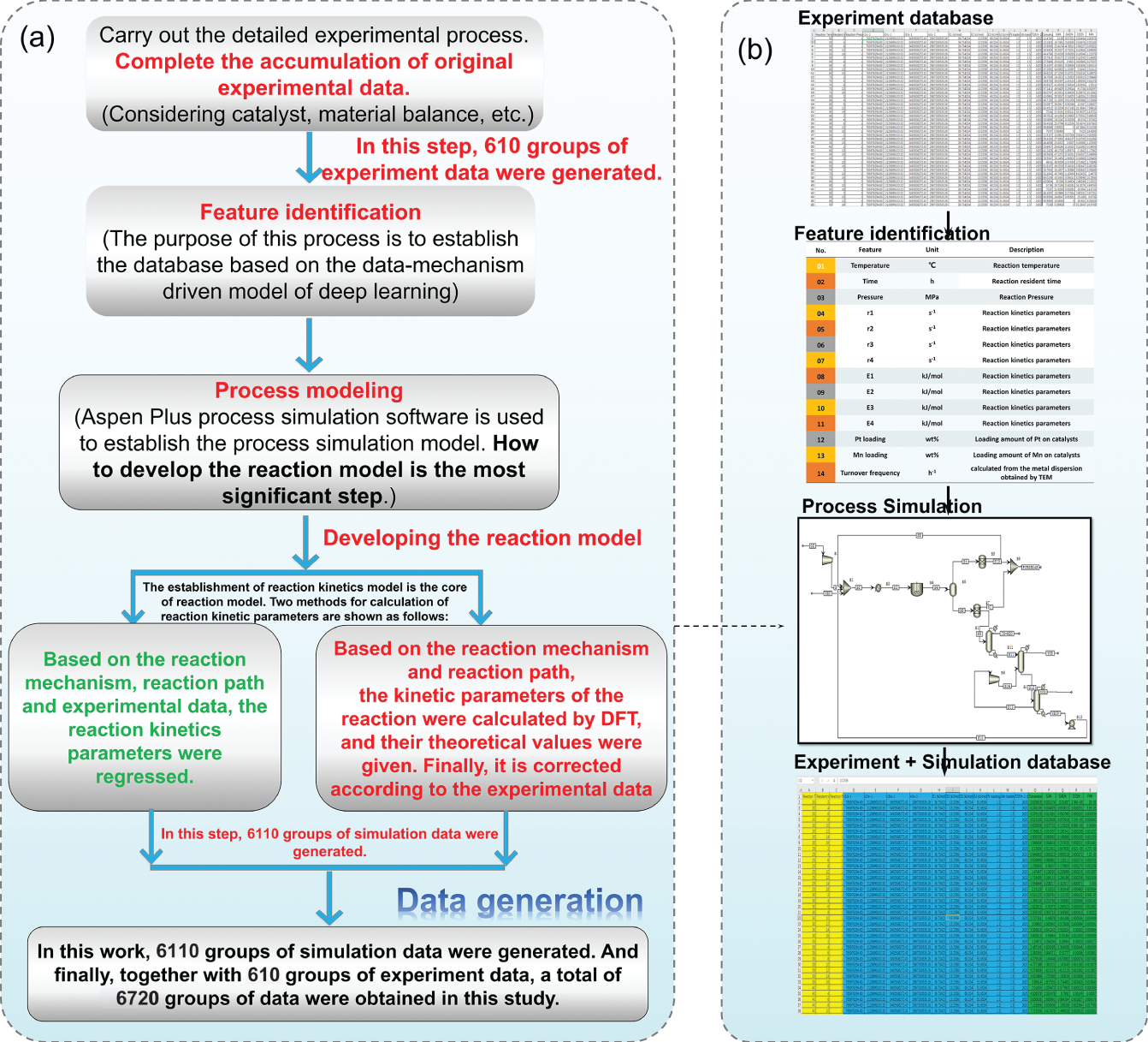
4.2.1 Database Generation
No.
Items
Unit
Description
F1
Temperature
°C
Reaction temperature
F2
Time
hour
Resident time
F3
Pressure
MPa
Reaction pressure
F4
E1
kJ mol−1
The reaction activation energy in the first reaction
F5
E2
kJ mol−1
The reaction activation energy in the second reaction
F6
E3
kJ mol−1
The reaction activation energy in the third reaction
F7
E4
kJ mol−1
The reaction activation energy in the fourth reaction
F9
Pt loading
wt%
Pt atom loading in PtMn/MCM-41 nanocatalysts
F0
Mn loading
wt%
Mn atom loading in PtMn/MCM-41 nanocatalysts
F10
TOF
h−1
Turnover frequency
F11
Conversion
%
The conversion of feedstock ethylene glycol
F12
GA yields
wt%
The yields of desired product glycolic acid
F13
GAD yields
wt%
The yields of byproduct glycolaldehyde
F14
CO2 yields
wt%
The yields of byproduct CO2
F15
FA yields
wt%
The yields of byproduct formic acid 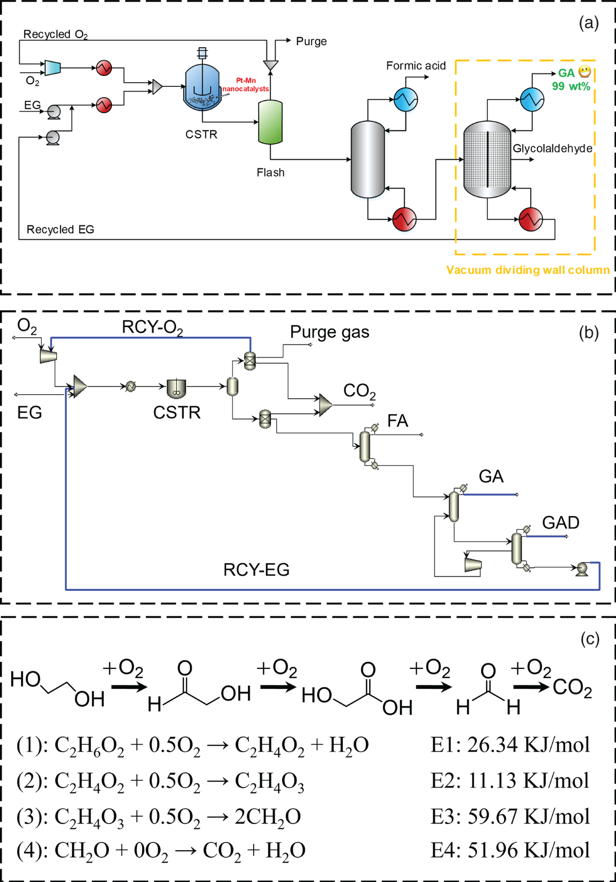
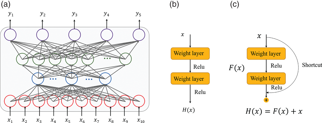
4.2.2 Deep Learning
4.2.2.1 Deep Neural Networks
4.2.2.2 Deep Belief Networks
4.2.2.3 Fully Connected Residual Networks
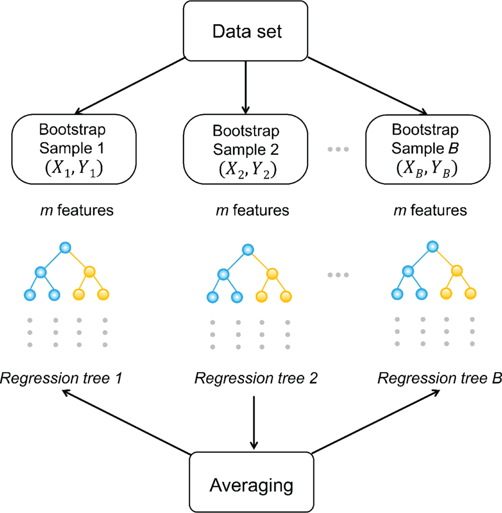
4.2.2.4 Random Forest
4.2.3 Optimization and Prediction
4.2.4 Life Cycle Multidimensional Evaluation
4.3 Results and Discussion
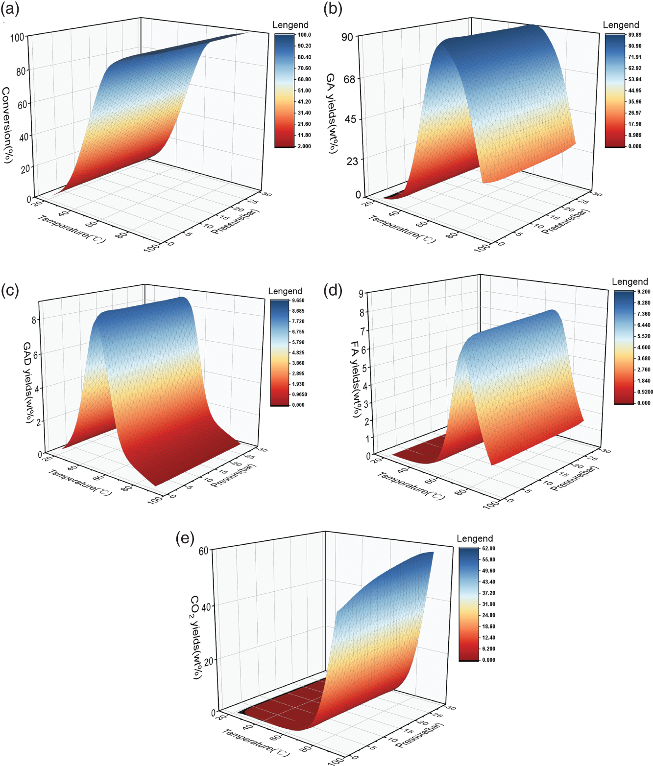
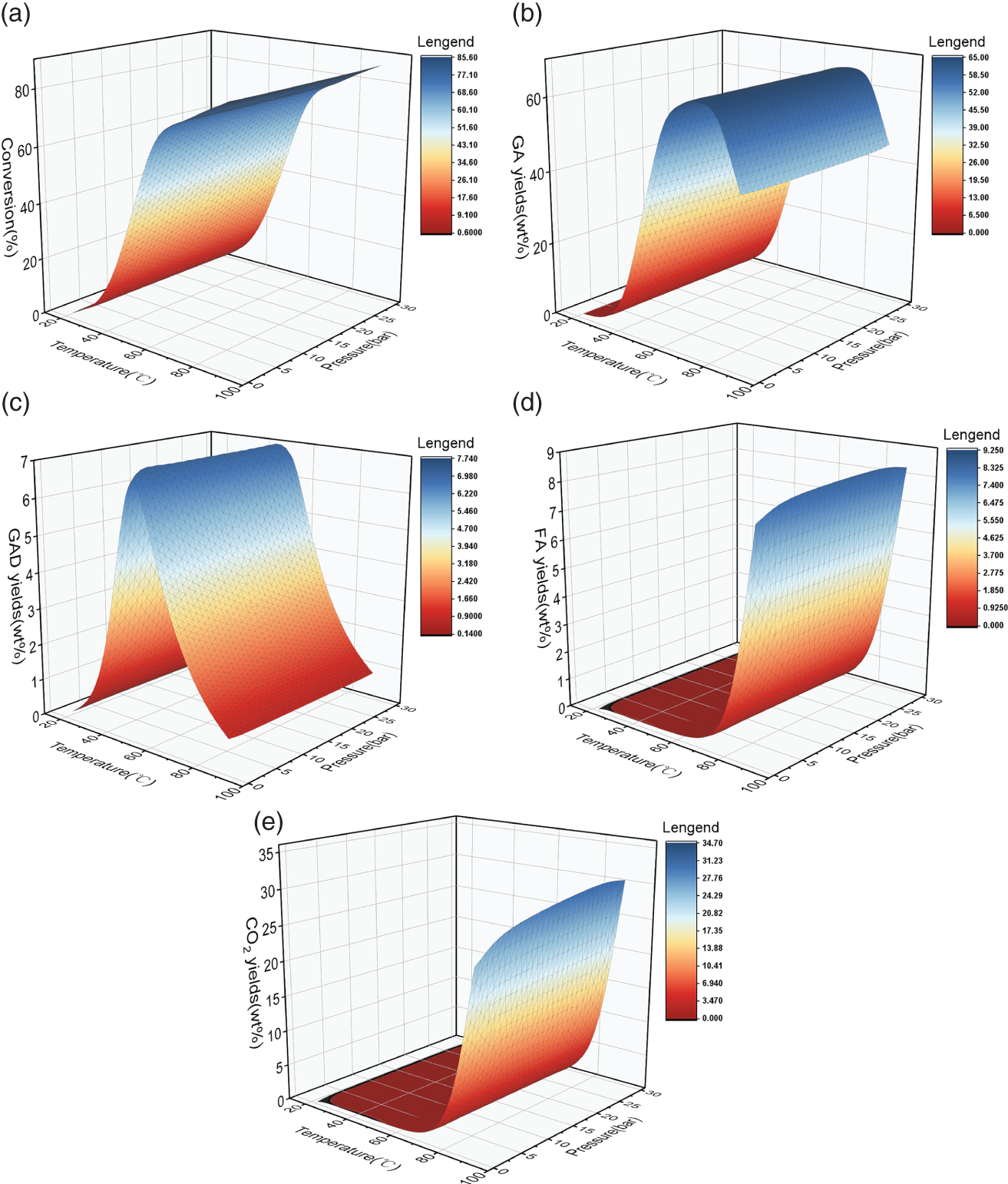
4.3.1 Data Analysis and Statistics Before Modeling
4.3.1.1 Analysis of Experimental Data
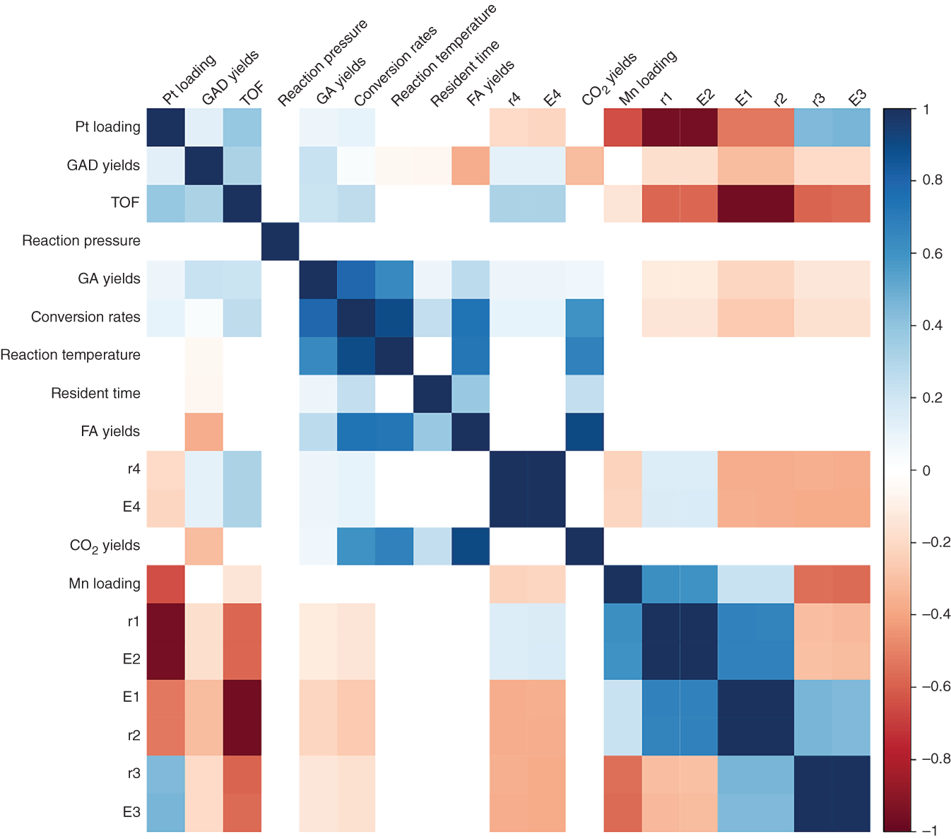
4.3.1.2 Data Dependence Analysis
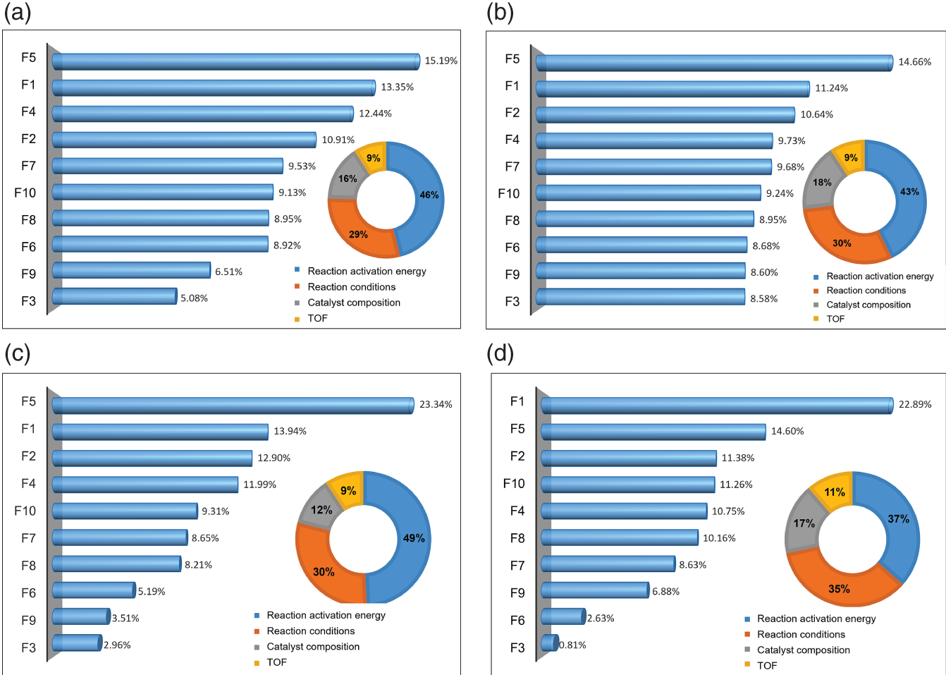
4.3.2 Model Comparison and Feature Important Analysis
4.3.2.1 Model Comparison
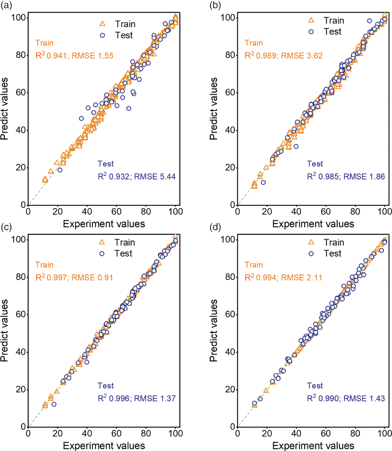

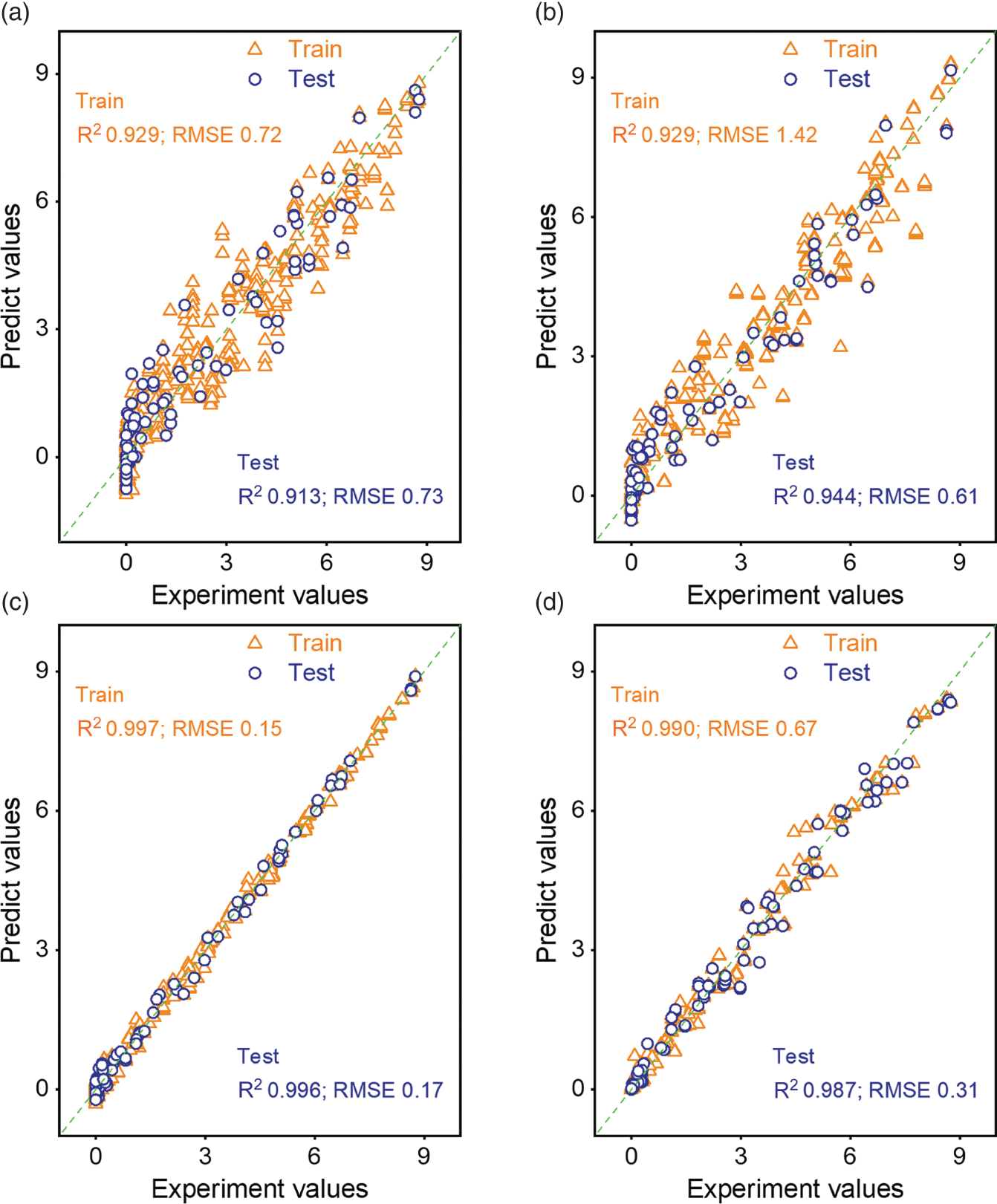
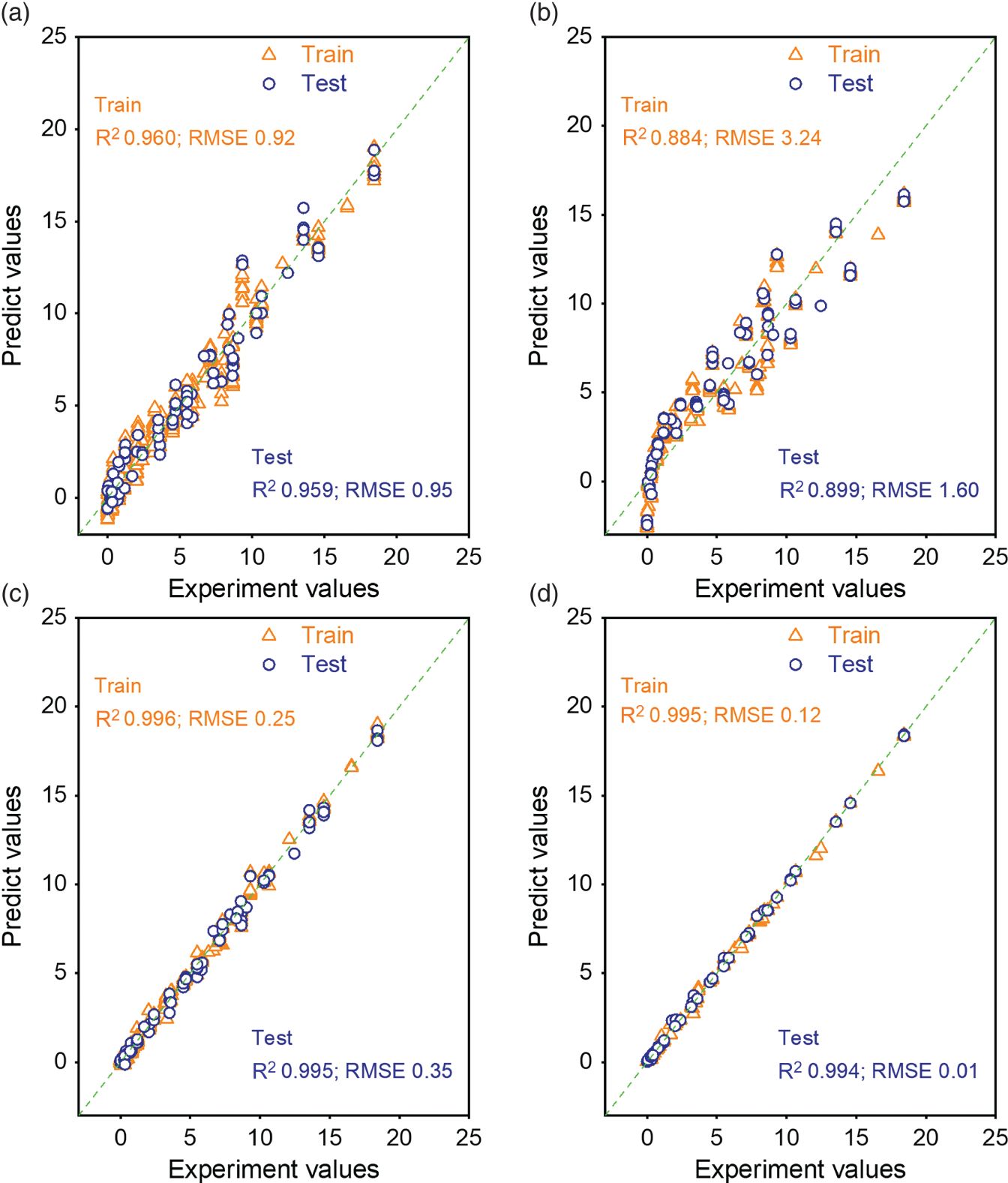
4.3.2.2 Feature Important Analysis

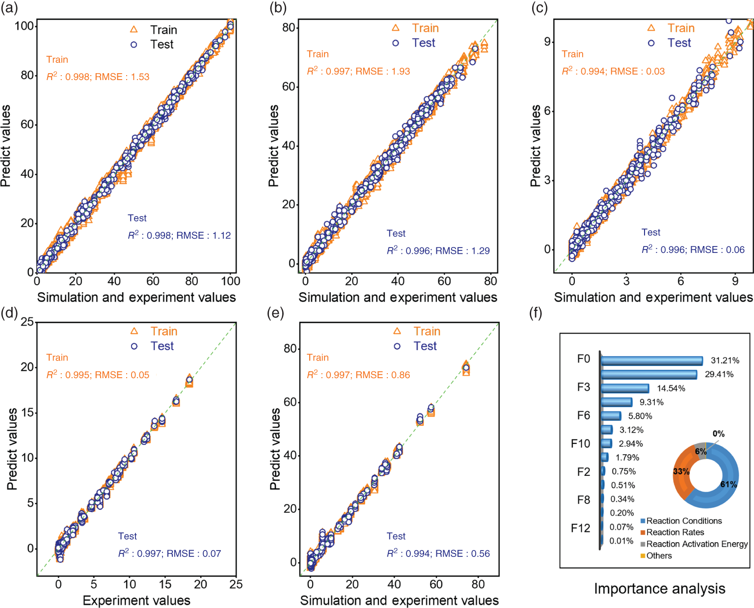
4.3.3 Performance and Feature Analysis of the Optimized FC-ResNet–GA Model
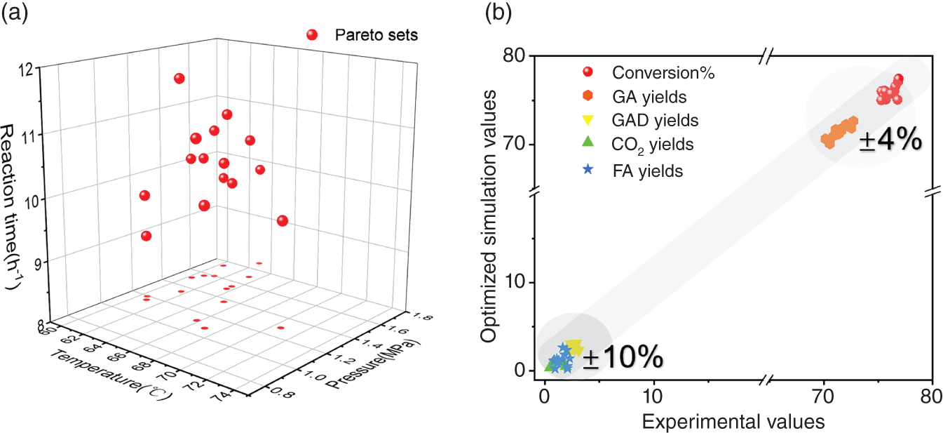
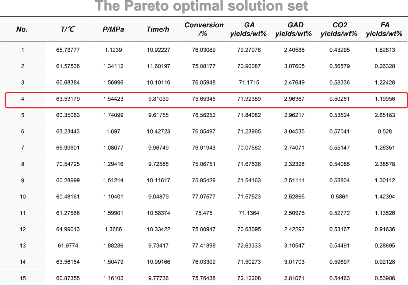
4.3.4 Process Multi-objective Optimization and Experimental Verification
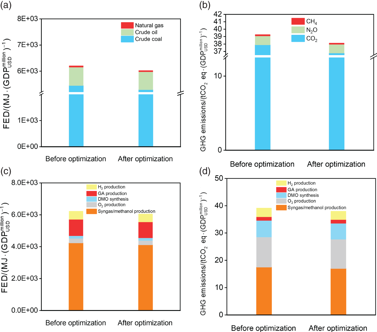
4.3.5 LCSA Based on the Optimized Parameters
4.3.5.1 Original Life Cycle Framework
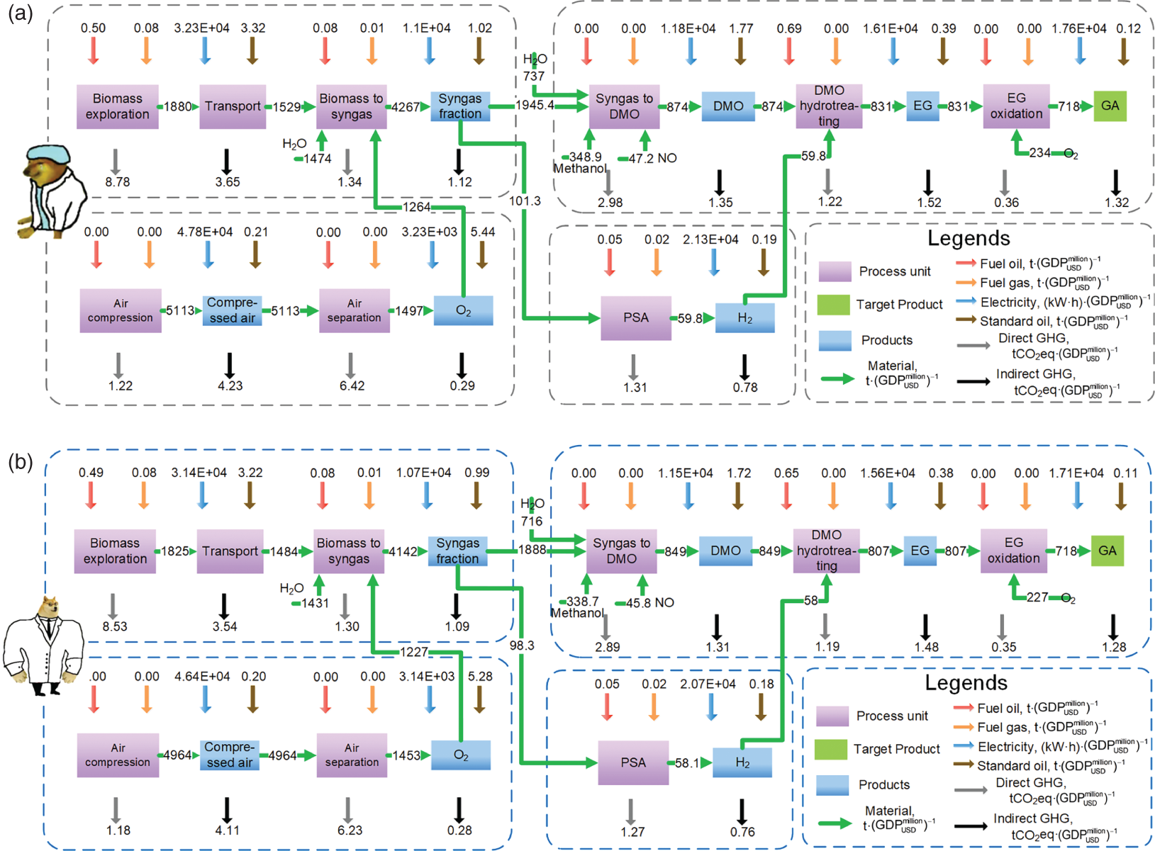
4.3.5.2 Life Cycle Inventory Analysis
4.3.5.3 Life Cycle Sustainable Interpretation and Assessment
4.4 Conclusion
4.A Pareto Optimization Set
4.B Experimental Data

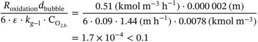
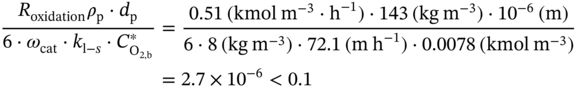
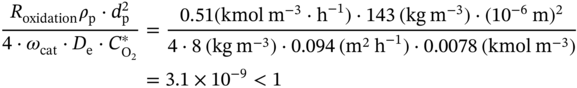
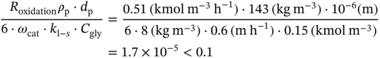
4.C Construction Method of Process Simulation Database Using Reaction Mechanism

4.C.1 Elimination of the Diffusion Limitations
4.C.2 Reaction Kinetics
References