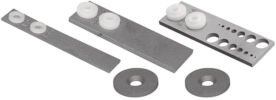
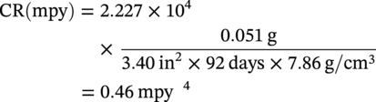
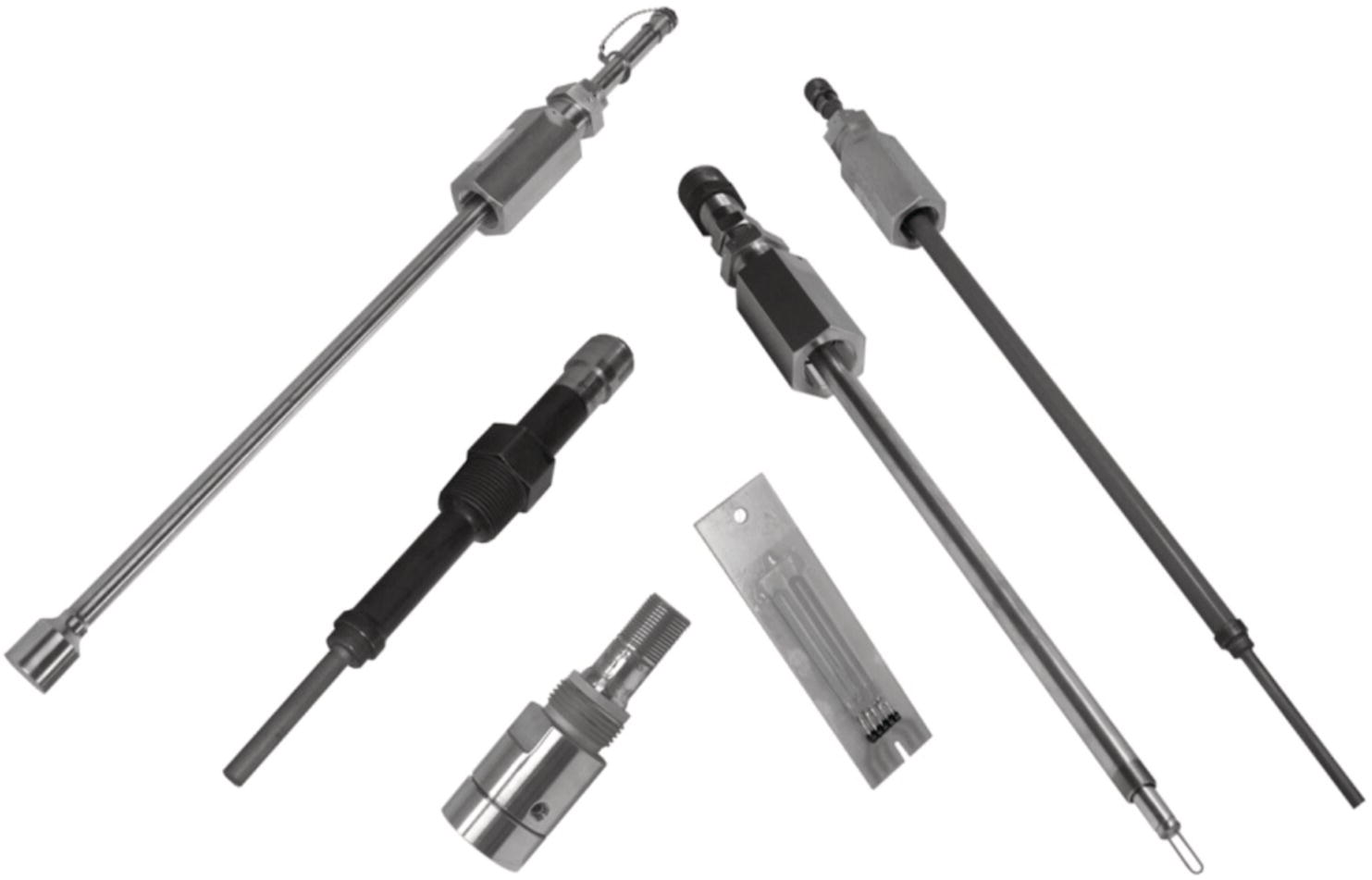
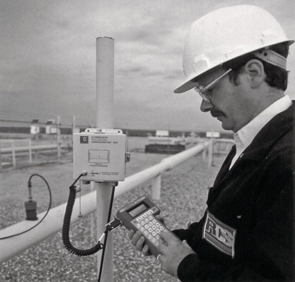
Daniel E. Powell* Williams, Tulsa, OK, USA The focus for this chapter is to provide an overview of the primary, most commonly used methodologies for monitoring potential corrosion within the interior of pipelines transporting crude oil, hydrocarbon liquids, or natural gas from production wellheads to the processing facilities, and ultimately to the customers. This monitoring enables us to detect potential threats of internal corrosion, as well as measure the effectiveness of any remediation measures, such as the application of corrosion inhibitor or biocide treatments. There are numerous books, reports, and standards that highlight corrosion monitoring as a tool for assessing and managing the integrity of pipelines. These include Corrosion Control in Petroleum Production [1], Uhlig’s Corrosion Handbook (Third Edition) [2], Field Guide for Investigating Internal Corrosion of Pipelines [3], NACE Internal Corrosion for Pipelines [4] manual, NACE Internal Corrosion for Pipelines—Advanced Course [5] manual, the internal corrosion direct assessment methodologies [6–8], as well as Preparation, Installation, Analysis, and Interpretation of Corrosion Coupons in Oilfield Operations [9] and Techniques for Monitoring Corrosion and Related Parameters in Field Applications (3T199) [10], which provide an overview of a number of monitoring techniques, providing the strengths and limitations of each. Our focus in this chapter is on the most commonly used and lowest cost monitoring techniques that are used worldwide, including those in remote locations, where telecommunications or electrical power may be limited. This chapter focuses on the use of mass loss coupons and electrical resistance (ER) corrosion probes, as those represent the most commonly used monitoring techniques. Although there may be specialized applications, such as the use of highly polished coupons that are used for evaluating and monitoring the effectiveness of mitigative measures, using electron microscopy, i.e., EM coupons. Such analysis is very labor intensive and expensive, and as such is primarily undertaken for specialized diagnostics or analyses. Again, the reader is referred to papers that address this specialized topic [11–14]. Although linear polarization resistance (LPR) corrosion monitoring is a common technique, our discussions in Section 28.2.2.7 will be somewhat abridged for two reasons. First, note that the internal corrosion monitoring discussed in this chapter is intended for the assessment of corrosivity within pipelines primarily transporting hydrocarbons, including crude oil, natural gas liquids, and natural gas, with relatively small proportions of produced or condensed water. Documents that discuss corrosion monitoring within pipeline systems transporting hydrocarbon have typically noted a limitation of LPR probes for this application [1, 10], citing “the need for a sufficiently conductive medium precludes the use of this technique for many applications in oil and gas, refinery, chemical, and other low-conductivity applications” [10]. Another limitation associated with such an electrochemical technique is the “bridging of electrodes with conductive deposits causes short circuits that affect results and can render them invalid until the electrodes are cleaned” [10]. Due to these perceived limitations, LPR probes are predominantly used in water handling systems for the crude oil and natural gas production and processing systems (including waterflood systems) and are ideal for such applications. There are other fine corrosion monitoring techniques, such as electrochemical noise (ECN or EN) [2, 10]. However, such monitoring systems require elaborate telecommunications systems, sophisticated data management, and skilled personnel to properly evaluate the data. Although EN monitoring systems have been successfully implemented at a few facilities, this technique has not been widely adopted. Instead, mass loss coupons and ER probes are still the most commonly used monitoring techniques used throughout the crude oil and natural gas industry for detecting and managing potential internal corrosion. This chapter has limited discussions regarding the use of ultrasonic thickness measurements as a method to measure internal corrosion rates. NACE International Publication 3T199 (2012) Techniques for Monitoring Corrosion and Related Parameters in Field Applications [10] cites that “the most commonly used techniques are mass loss coupons, ER probes, linear polarization probes, and ultrasonics.” The ultrasonic thickness measurements serve as a direct, nonintrusive technique for measuring metal thickness and calculating corrosion rates. Section 3.1.1 of the NACE 3T199-2012 publication states that ultrasonics “is normally used for corrosion prediction over long periods of time and is not suited for monitoring real-time corrosion rate changes.” This publication of 3T199-2012 also states in their Section 3.2.2 and 3.2.3 for flaw detection and flaw sizing, respectively, that ultrasonics “does not quantify as a corrosion monitoring technique” [10]. This was reaffirmed in the NACE TR3T199-2020 update, under their Section 4.2.2, Limitations, Note “e” [10]. A published paper from NACE Corrosion 2012 reviewed “Nonintrusive Techniques for Monitoring Internal Corrosion of Oil and Gas Pipelines”, concluded that “ultrasonic handheld appears to be the most ideal nonintrusive technique currently,” and noted a limitation associated with liquid couplant drying out [15]. This paper also pointed out that the handheld ultrasonic testing (UT) can reliably measure pits with an error of ±0.01 in. (±0.25 mm) and is capable of detecting the location of a defect or pit. Thus, based on the NACE publication 3T199 and the published paper [15], the ultrasonic wall thickness measurement serves as an excellent tool for inspecting pipe wall and assessing the integrity of pipelines, but cannot offer the precision over a short period of time for closely monitoring corrosion rates and assessing the effectiveness of remedial measures, such as chemical treatments. We will also have only limited discussions regarding the use of in-line inspection (ILI) data from intelligent pig runs through pipelines. First, a separate chapter, Chapter 29, will discuss ILIs. Second, although many people may view ILI as a monitoring technique, it is actually an inspection technique and does not have the same sensitivity as monitoring instrumentation placed within the pipeline. ILI runs through individual pipelines are typically several years apart, and there are also limitations in the precision of individual measurements versus those from coupons or electronic probes placed within a system. (This will be discussed later in this chapter.) Due to the limited precision and long duration between ILI runs, results should not be used as a basis for controlling remedial measures, for example, chemical treatments, when other internal corrosion monitoring methodologies, such as coupons or electronic probes are available. Nevertheless, corrosion specialists should review any and all ILI data as part of the overall integrity assessment and evaluating potential internal corrosion. Again, the purpose of this chapter is to provide the reader with a practical perspective for the most commonly used, most cost-effective approach to detecting and controlling potential internal corrosion in crude oil and natural gas gathering systems, processing facilities, and the piping to the customers. The key is to place the monitoring instrumentation along the path where any free water would be swept. We will then present a strategy by which these monitoring results are used to trend corrosion rates and “drive” remedial measures, such as corrosion inhibitor or biocide treatments. Finally, we will present an overview of the relative ability of mass loss coupons or electronic probes to detect active corrosion, versus inspection techniques such as ultrasonic wall thickness measurements (UT), radiography (radiographic testing [RT]), or magnetic flux leakage (MFL). It will be apparent that mass loss coupons or electronic probes placed within the process systems offer the best option for detecting and controlling potential internal corrosion, and thus helping to maintain the system integrity. Corrosion is the deterioration of a material, usually a metal, that results from a reaction with its environment [7]. As applied to the oil and gas industry, corrosion is the unwanted deterioration of the piping or process equipment associated with (1) crude oil or natural gas gathering systems, (2) the production or processing facilities, any water or gas injection systems used to enhance production, (3) the export or sales lines, and (4) distribution systems. If the corrosion processes continue untreated, the cumulative effect could initiate sufficient deterioration that would affect the integrity of the piping or process equipment, and possibly result in failure. In the following sections, we will present an overview of internal corrosion monitoring, based on the use of corrosion coupons or electrical probes (primarily ER) probes for detecting corrosion. (These are the most commonly used monitoring tools per NACE 3T199 [10] for pipelines transporting liquid or gaseous hydrocarbons.) Strengths and limitations will be noted. Next, we will present the placement of the corrosion monitoring within the process streams and in particular the pipelines. “Placement” addresses not only the axial position within a pipeline, but also the optimum orientation or azimuth for installing corrosion monitoring instrumentation. We will then present a strategy for applying chemical treatments, primarily corrosion inhibitors, such that corrosion rates can be kept low, and the designed service life can be achieved. Next, we will compare the relative sensitivities of nondestructive inspection techniques, such as ILIs, radiography, and ultrasonic inspections versus corrosion coupons or electronic probes to detect the onset of corrosive conditions. Finally, we will have a brief discussion related to the comparison of the most recent nondestructive testing (NDT) inspection data (Section 28.6) and/or fluid sample analysis (Section 28.7) to the most recent internal corrosion monitoring results. The assessment of the trends would serve as an independent check to verify or confirm internal corrosion monitoring results. Collectively, this approach should provide the reader with a comprehensive overview of internal corrosion monitoring, and how to use those results to maintain system integrity. Internal corrosion monitoring is the tool used by corrosion professionals to detect the onset of corrosive conditions. The discussions will be focused on monitoring corrosion rates for crude oil, hydrocarbon liquids, and natural gas in gathering pipeline, production facilities, and sales or export/transmission pipelines to the customers. Our focus will be on the use of mass loss coupons and ER corrosion probes that are placed within pipelines. These are the primary “workhorses” of the oil and gas industry. However, the monitoring techniques discussed can also be used in other industries, such as the chemical industry, water processing, etc. In Section 28.7, we will briefly discuss fluid sampling analysis, which complements the metal coupon and electronic probe measurements of corrosion rates, and should provide independent confirmation of the onset of internal corrosion. The most obvious question is “Why does the oil and gas industry place such a priority on the use of metal coupons and ER probes, as opposed to the use of (a) nonintrusive techniques, such as ultrasonic wall thickness measurements or radiography, (b) comparatively modern monitoring techniques, such as EN or ECN, or, (c) others, such as the use of EM coupons?” First, we need to define “intrusive” and “nonintrusive.” Please refer to Section 28.9, which provides definitions from NACE’s 3T199 [10]. “Intrusive” monitoring requires the monitoring coupon or electronic probe to be placed directly within the test environment, for example, within the pipeline. In contrast, “nonintrusive” monitoring is a measurement from the outside of the pipe or vessel, such as a measurement of the remaining thickness of the pipe wall. Generally, corrosion engineers prefer monitoring results from coupons or probes placed directly within the test environment or process stream. However, if those results are not available, monitoring results from nonintrusive techniques would become the primary analytical tool. Here are a few considerations that highlight why mass loss coupons and electronic probes are the most widely used monitoring tools—particularly for remote locations or when cost considerations may limit monitoring options: Consider mass loss metal coupons first. The vast majority of pipelines found in gathering systems, processing facilities, or transmission pipelines are constructed of carbon steel. Accordingly, one of the most commonly used internal corrosion monitoring techniques is based on inserting carbon steel mass loss coupons into the process stream for a set period of time, for example, 90 or 180 days, and then removing and cleaning them to remove any corrosion products. The reduction in mass over the exposure period is used to determine the internal corrosion rate. If pits are observed within the metal coupons at the end of the exposure period, then a pitting rate would be based on the depth of the deepest pit and the exposure period [4, 9]. (If we are to monitor corrosion rates within a section of a gathering pipeline or piping within a production facility, which has a different metallurgy, the corrosion monitoring should be based on that metallurgy. For example, coupons used to monitor a pipeline constructed with duplex stainless steel should be made from the duplex stainless steel. The companies that provide metal coupons or electrical probes for corrosion monitoring will typically offer to fabricate coupons or electronic probes using whatever base material is required to match system metallurgy. However, there is likely to be a premium charge for the customization.) Figure 28.1 illustrates the variety of metal coupons that are commercially available. It is fairly straightforward to determine general corrosion rates from metal coupons removed from the system. We will start with a known initial mass for the coupon. The coupon will also have a known geometry, whether it has a rectangular shape, a cylindrical shape, or appears like a round washer. The initial dimensions of the metal coupon will determine the total surface area exposed to the environment being monitored. The density of the material, which is the mass divided by volume, is known. The date or time the metal coupon was installed within the system, and the date or time that the metal coupon was removed from the system, are also known. Finally, we measure the weight of the coupon after it has been removed from the system. The weight of most interested in is the final weight, after any deposition and corrosion products have been removed. (It may also be useful to document the appearance of the coupon as soon as possible after the coupon is removed from service, including the color and depth of any deposits or corrosion products.) From the already mentioned data, we can then calculate the corrosion rate. Figure 28.1 Manufacturers offer a variety of styles of metal coupons for monitoring internal corrosion. The coupon on the right is used to detect scale depositions. (Courtesy of Rohrback Cosasco Systems.) NACE SP-0775-2013 (or the most current year) provides several equations for determining corrosion rates [9]. The basic formula for the corrosion rate in mils per year (mpy) or in mm/year is where To report corrosion rates in mpy, use where To report corrosion rates in mm/year, use where Note that corrosion rates, which could be reported in mm/year, may also be reported in μm/year: The factors in Equation (28.1a and b) are derived from the conversion factors, such as inches to centimeters, millimeters to centimeters, inches to mils, and days to years, to generate corrosion rates in mpy or mm/year. For calculating general corrosion of coupons, we make the fundamental assumption that the exposed surface area remains constant, and the only thing that changes is the relative thickness of the coupon. Consider as an example, a carbon steel coupon, which had a 0.0510 g mass loss over a 92-day exposure. Also, note that the steel has a density of 7.86 g/cm3. Assume an exposed surface area of 3.40 in.2. For this example, we want to determine corrosion rate in mpy, where 1000 mils = 1 in. Here is an example of how the corrosion rate is calculated In this example, the calculated corrosion rate is 0.462 mpy, which is well below a generally accepted maximum acceptable corrosion rate of 1.0 mpy, as per NACE SP-0775-2013 [9]. When corrosion coupons are placed within pipelines, it is possible that pits may form on the metal coupons, just like they could form on the base metal of the pipe. If left unchecked, pits in pipelines could develop and grow to the point of penetrating through the wall thickness, and could result in a leak. Accordingly, an inherent point of internal corrosion monitoring is to check the metal coupons for the evidence of pit formation. Note that pits could form for many different reasons, whether from microbiological results, such as the action of sulfate-reducing bacteria (SRB) or acid-producing bacteria (APB), oxygen ingress, H2S, or perhaps from the presence of carbon dioxide, which reacts with water to form carbonic acid. As in the case of determining general corrosion rates, the first step is to clean the coupons by removing any corrosion products from the surface of the metal coupons. Then, the depth of individual pits can be measured either through the use of a light microscope or by using a needle gauge and comparing that reading to one taken on unaffected base metal. There are also developing technologies that are just being introduced in 2013, which use laser or three-dimensional structured light to profile pits. These new pit depth/profile technologies are expected to become more widely used in future applications due to the reduced time required for each assessment [16]. Although the depth of the deepest pit is of the greatest interest, it should also be noted whether the pit was an isolated pit, or if there are numerous pits in close proximity, for example, a network of pits. Unlike laboratory work, the analysis of pitting observed on metal coupons must rely upon some basic assumptions. We know when the coupon was installed, when it was removed, and we also know the depth of the deepest of all the pits. However, we do not know the specific date the pit initiated. Hence, determination of a pitting corrosion rate has to be made based on the date of installation. NACE SP-0775-2013 presents a listing of general corrosion rates and pitting corrosion rates, categorizing them as “low,” “medium,” “high,” and “severe” [9]. These are presented in Table 28.1. We use this table as a guideline for defining acceptable and unacceptable corrosion rates. We would take the worst, highest general or pitting corrosion rate for any individual corrosion coupon, and use that value to categorize the observed internal corrosion. If the categorization is above acceptable limits, that would be used as a basis for adjusting chemical treatments or other mitigative measures. (These are discussed in Section 28.4.) Table 28.1 Categorizing Carbon Steel Corrosion Rates for Oil Production Systems [9] Source: NACE SP-0775-2013. mm/year = millimeters per year, mpy = mils per year (1000 mils = 1 in.). Before leaving this topic, we should note that the maximum acceptable corrosion rate is really based on the remaining corrosion allowance of a pipeline and the projected service life. Pipelines are designed to have a certain wall thickness, which is required for pressure containment. This portion of the pipe wall thickness is based on the maximum allowable operating pressure (MAOP). The additional portion of the wall thickness is the allowance for corrosion. Corrosion professionals use this additional wall thickness (that beyond the thickness required for pressure containment) and the projected remaining service life to determine the maximum acceptable corrosion rate. A pipeline that has experienced very little corrosion throughout most of its service life may have sufficient additional wall thickness (beyond that thickness required for pressure containment) to allow acceptable corrosion rates to exceed the 1.0 mpy (0.025 mm/year) guideline late in its service life. In contrast, a pipeline that has operated under more severe conditions and has only a small remaining corrosion allowance might have a maximum acceptable corrosion rate below the 1.0 mpy (0.025 mm/year) guideline late in its service life. (Another option for pipeline and corrosion engineers to consider is reducing the MAOP for the section of pipe. That would reduce the portion of the pipe wall thickness required for pressure containment, but would increase the portion of the pipe wall thickness for the corrosion allowance. However, this option should only be used very judiciously.) ER probes are very valuable tools for measuring internal corrosion rates without having to physically remove the sensing element from the process stream. The corrosion control professional can simply go to the location of the ER probe and make an electronic connection to the probe or remote data logger, and record or download the data, which would then be taken to an office for assessing the corrosion rate trends. Figure 28.2 illustrates several styles of ER probes used to monitor internal corrosion within the field and will be discussed in more detail momentarily. Figure 28.3 illustrates how corrosion rate measurement data can be retrieved “from the field” through a handheld data logger. (Intrinsic Safe Data Loggers are commercially available for collecting or downloading data in hazardous environments.) All ER probes use measurements of the resistance of the sensing unit to quantify the internal corrosion rates. Internal corrosion mechanisms cause the resistance of the probe’s sensing element to change (increase). Hence, the internal corrosion rate can be determined from successive measurements of the resistance of a wire loop, strip, or cylindrical element style ER probes versus time. The “raw data” from ER probes reflect the cumulative general corrosion on the probe’s sensing element, including the effects from any short duration transient event that may have occurred between readings. Thus, like metal coupons, ER probe measurements reflect cumulative corrosion, and the consequences of any transient corrosive events, which might occur between readings, will not be missed. Figure 28.2 Various corrosion probe designs. (Courtesy of Rohrback Cosasco Systems.) Figure 28.3 ER probe connected to remote data collector. Note the cable connected to a probe located on top of this pipe. The cable connects to a remote data collector, which can be programed to measure the corrosion rate at regular intervals, such as every 15 min, hourly, daily, weekly, and so on. When the handheld device is connected to the remote data collector, the archived data can be retrieved for analysis. Such a data collection system is beneficial for remote locations typical of the oil and gas industry. However, for monitoring corrosion rates near compressor stations or processing facilities, it may be more beneficial to connect the electronic probes to the facility’s SCADA systems. (Courtesy of Rohrback Cosasco Systems.) Note that ER probes are designed to measure general corrosion rates, rather than pitting corrosion rates. If pits form on the sensing element, it will be obvious that this data is invalid, since successive readings typically follow an exponential curve. When such behavior is observed, the ER probe should be replaced. Temperature effects are minimized by a second, protected element within all ER probes. Readings from the protected element are compared to those from the exposed element, thereby providing the basis for calculating the “true” metal loss and corrosion rate. Note that probe design is critical for obtaining valid monitoring results, and details can be found in technical literature provided by the probe manufacturer. If electrical probes are covered by conductive corrosion products or deposits, the probes would not be able to accurately measure corrosion rates. (Presumably, the pipe walls would be in a similar condition.) The following sections describe the most common types of ER probes. These are the wire loop, tubular type, tube type, spiral type, and flush type probes. Each has a different surface area, sensitivity, and effective probe lifetime. Figure 28.4 depicts the appearance of several styles of ER corrosion probes. Probe manufacturers often use a letter to indicate the different types of probes, such as W for wire, T for tubular or tube, F for flush probe, and so on. The numerical value following the letter designation indicates the relative thickness of the sensing element, which indirectly provides the effective service lifetime of the probe. Figure 28.4 Various styles of ER probes. (Courtesy of Rohrback Cosasco Systems.) As an example, a T10 probe would be a tubular type probe, which would have an effective lifespan of Wire loop ER probes are commonly used due to their high sensitivity. Basically, they appear to have what appears to be a simple wire loop extending from the end of the probe into the system being monitored. Wire loop probes appear like the probe on the left in Figure 28.4. These probes provide a high sensitivity for detecting the onset of corrosive conditions and are very useful when first assessing corrosion rates within a new pipeline or when conducting performance tests, such as for the selection of new corrosion inhibitor products. However, the temperature stability of wire loop ER probes can be relatively poor, and the probe elements are subjected to premature failure (due to fatigue) under high flow rates or when particulates such as sand or formation fines are transported through the pipeline and strike the sensing element. Velocity shields are recommended to help protect the sensing element of wire loop ER probes. Wire loop ER probes can be used in small diameter pipelines, or can be located near pipe walls. A variety of sizes for the wire elements are available, each offering a trade-off between sensitivity and the service life of the probe. Probe response time charts are available from the probe manufacturers. As an example, those charts would show that for a 10 mile (254 μm) span wire loop probe, it would take approximately 100 h or approximately 4 days to detect a 10 mpy (254 μm/year) corrosion rate. Those charts also show that it would take approximately 8 days to detect a 5 mpy (127 μm/year) change in corrosion rate, and a bit over a month to detect a 1 mpy (25.4 μm/year) corrosion rate. These response times are very short compared to the typical 90-day exposure cycle for mass loss coupons. That provides an insight regarding why wire loop ER probes are often used when first establishing baseline corrosion rates and setting the chemical treatment rates. Note that wire loop ER probes are susceptible to iron sulfide bridging, which may occur within sour systems. “Bridging” refers to the deposition of iron sulfide, which creates temporary low-resistance pathways across the deposition (“bridge”). When the deposition is on the sensing element (here a wire loop ER probe), the new electrical path will render measurements invalid. Hence, wire loop ER probes should not be used in sour service. Tubular loop probes are very similar to wire loop ER probes. They use capillary tubes instead of wires as the sensing element; see Figure 28.4. The sensing element is quite weak but is very sensitive due to the 0.004 in. (101.6 μm) wall thickness of the capillary tube. Tubular loop ER probes are normally used with velocity shields and are placed in low shear rate environments. Like wire loop ER probes, tubular ER probes are prone to premature failure due to fatigue at the base of the element, where the capillary tube extends from the end of the probe. Velocity shields may help reduce fatigue and premature failure of the capillary tubes due to fluid flow. Tubular loop ER probes are also subjected to sulfide bridging if the probe is installed in sour service. Hence, they are not recommended for that service. Since tubular ER probes are able to detect corrosion rates as small as 1 mpy (25.4 μm/year) in 10–12 days, they are also commonly used when first measuring the corrosion rates within a pipeline. They may also be used when conducting performance tests for selecting new corrosion inhibitor products. Tube or cylindrical ER probes have a large surface area and a stout design. They appear like tubes or cylinders, as depicted in Figure 28.4. These stout probes have a high resistance to premature failure and are designed for environments having potentially high corrosion rates, including locations where there may be significant corrosion or erosion. Tube ER probes would be the probe of choice for oil production pipelines having high flow rates. The tube or cylinder-shaped ER probes are also less susceptible to sulfide bridging and can be used for monitoring corrosion in sour service. They should have relatively long service lives when placed in environments having relatively low corrosion rates. The tube type ER probes appear like solid cylinders and are available in various element sizes, such as 0.01 in. (254 μm), 0.02 in. (508 μm), and 0.05 in. (1270 μm) elements for effective element thickness of 0.005 in. (127 μm), 0.010 in. (254 μm), and 0.025 in. (635 μm). It would require a T10 probe (0.010 in. [254 μm] effective element thickness) approximately 25 days to detect a 1 mpy (25.4 μm/year) corrosion rate. Flush mounted probes are designed for placement into pipelines or vessels without protruding beyond the wall thickness. The two probes on the right side of Figure 28.4 depict a top view of two different designs for the sensing elements of flush mounted ER probes. Unlike intrusive probes, which extend partway into the diameter of a pipeline, flush-mounted probes are even with the pipe wall and can be left within pipelines while the pipeline is mechanically cleaned by pigs. There are advantages and disadvantages with each design. The size of the sensing elements may be restricted, due to the size of the access fitting. The most common flush mounted probes are the F5 and F10 models, which offer between 5 and 10 mile (127 and 254 μm) range or span for cumulative corrosion measurements. (Thicker elements have been made, but have been less effective for the corrosion rates normally encountered in the oil and gas industry.) For most oil and gas applications, the optimum flush mounted probe would be a flush mounted probe having a 5 mile (127 μm) range or span, which is oriented at 6:00 o’clock on horizontal section of piping. It would require approximately 10–12 days to detect a change, based on a 2 mpy (50.8 μm/year) corrosion rate. When used in sour service, flush mounted ER probes, which have a sensing element with a spiral or complex design, are susceptible to sulfide bridging. If the sensing element is in the shape of a rectangle, it will have a very short resistance path and a very low resistance. However, probes with that design have a high “noise” level, which means a longer response time is needed to separate the true signal from “noise.” Consequently, regardless of the design of the probe element, flush mounted ER probes are not recommended for monitoring within sour service conditions. Instead, it would be more advantageous to use high-resolution ER techniques for such a specialized application. High-resolution ER probes (Figure 28.5) are “enhanced” ER probes, which provide metal loss data that can be converted to corrosion rates. These probes use a similar method of measurement compared to the conventional ER probe, but provide significantly improved compensation for temperature changes. Modifications to instrumentation and probe design have also contributed to significant improvements in electronic noise reduction and enhanced measurement resolution. High-resolution ER probes are commercially available. The probes must be continuously monitored, using either a data logger or an online data collection system. Higher resolution allows trend information to be collected in a shorter period. High-resolution ER probes perform well in sour service conditions (2–10% H2S), where iron sulfide bridging could occur, and most conventional probes would be inoperable. Figure 28.5 High-resolution ER probe. Note the electronic package above the corrosion probe’s sensing element. This helps to reduce/enhance the signal-to-noise ratio, improving the resolution. (Courtesy of Rohrback Cosasco Systems.) According to product literature, the sensitivity of high-resolution ER probes can be as low as 2 × 10⁻⁷ mm (0.2 μm = 0.0079 mils). The main application for these probes would be in oil and gas gathering systems, where corrosion rates would be expected to be approximately 1–3 mpy (25–76 μm/year). LPR probes use a totally different technique for measuring corrosion rates than is used by the ER type probes. Unlike the ER probe, which uses two or more successive readings of the probe’s resistance to calculate a corrosion rate, each LPR measurement of the corrosion rate is independent of previous readings. LPR readings are essentially “real-time” measurements of corrosion and cannot detect any transient corrosive conditions, which may have occurred between LPR readings. Consequently, the time between readings needs to be very much shorter than for ER probe readings to be able to detect corrosion associated with transient conditions. There are two basic designs of the LPR probe, namely, the three-electrode and two-electrode designs. Figure 28.6 depicts a two element LPR corrosion probe. For each type of probe, a fixed potential difference is established between the electrodes, and the resulting current is measured. At the low potential differences used in this polarization technique, the corrosion rate is proportional to the corrosion current. (A detailed explanation of linear polarization techniques is available from LPR manufacturers.) Figure 28.6 The two-electrode LPR probe. (Courtesy of Rohrback Cosasco Systems.) The three-electrode LPR probe used to be superior to the two-electrode probe, since the three-electrode LPR probe could better compensate for IR drops in low-conductivity fluids. However, for the last 20 years, instruments have been commercially available that compensate for IR drop by using a DC measurement plus high-frequency AC compensation. Hence, the issue of using either a two- or three-electrode LPR probe is no longer relevant. LPR techniques should be used for measuring general corrosion—not pitting corrosion. The LPR technique requires conductive solutions around the electrodes and works best when the solution is hydrocarbon free [10]. LPR probes have historically not been recommended over ER probes for measuring corrosion rates in oil or gas systems, which are predominantly hydrocarbon based, and have low water cuts [10]. The hydrocarbons tend to film or coat the electrodes, lowering the electrical conductivity. Also, if the sensing elements are coated with iron sulfide (FeS), there could be a bridging between the elements, which could also distort or invalidate the results. Consequently, there should be limited usage of LPR probes in sour environments [10]. However, LPR probes are great for water applications, such as water processing or water injection systems that are hydrocarbon free. “Garbage in, garbage out” is a commonly used adage to emphasize the importance for obtaining good—valid—data. It also applies to the collection of internal corrosion monitoring data. Many pipeline and facility designers make the assumption that the flow through a pipeline is a homogeneous mixture. When access fittings for internal corrosion monitoring coupons or electronic probes are placed within systems, they are often placed at convenient locations—not at locations or orientations, where internal corrosion is most likely to occur. In this section, we will describe the strategies for placing the internal monitoring weight loss coupons or electronic probes within pipelines. First, we will discuss where along the length of a pipeline the monitoring should be placed, and then we will discuss the orientation of that monitoring. Consider a major trunk line or pipeline segment having no other pipelines flowing into or out of the pipeline. Liquids or gas entering the pipeline will also exit the pipeline. Thus, we have a system, such as depicted in Figure 28.7. For this illustration, we have a starting point, where the trunk line departs from a pad containing numerous producing wells, and then flows to a crude oil or natural gas processing facility. Two monitoring points are illustrated in Figure 28.7. One monitoring location is at the beginning of the line and just upstream of the chemical injection point. This location could be used for obtaining baseline internal corrosion rates. The second location is at the end of the pipeline just upstream of the gathering facility. The second is the more important of the two monitoring points, as it provides the internal corrosion rate for the pipeline and provides a measure for the effectiveness of corrosion inhibitors in controlling (minimizing) internal corrosion. The strategy is that regardless of how corrosive the liquids or gas entering the pipeline, the corrosion inhibitors injected at the start of the pipeline should be adjusted to a sufficient chemical injection rate to attain acceptable corrosion rates at the end of the pipeline. The point is to ensure there is sufficient chemical remaining within the process stream at the end of the pipeline to protect the base metals and that it had not been consumed upstream of that monitoring point. Figure 28.7 Ideal location for monitoring internal corrosion. (References [17, 18]/with permission of NACE International.) Figure 28.8 Location of internal corrosion monitoring near the end of one subsea pipeline. (References [18, 19]/with permission of NACE (National Association of Corrosion Engineers).) Let us consider a real-world example from Southeast Asia. Production from a number of wells on one offshore platform fed a pipeline that transported wet (saturated) gas to a second downstream platform. Figure 28.8 illustrates the monitoring point on the downstream platform and represents the end of that pipeline, before the production was comingled with any other production. Note that the internal corrosion monitoring probe was installed through an existing fitting on the piping at this downstream platform. Besides for being at the end of the pipeline, the monitoring point was also in a (relative) low point on the process stream, where any free water (produced or condensed) could accumulate. Thus, the monitoring would be at a point where water could accumulate, and internal corrosion is more likely to occur. Before discussing the monitoring results, we should bring to the reader’s attention the internal corrosion direct assessment methodologies [6–8]. Modeling is a key to knowing where any liquids could accumulate in pipelines transporting natural gas. These “hold up” points are ideal locations for monitoring any potential internal corrosion, provided they are accessible. (The reader is referred to the NACE direct assessment standard practices and models.) For the piping depicted in Figure 28.8, we note that the gas flow came from a subsea pipeline that ran to the base of the offshore platform, followed by a vertical riser, a short horizontal run, and then a short dip to the horizontal section depicted in the figure. Thus, the line had an obvious low point, which was easily accessible and where any liquids would (briefly) accumulate, before those liquids were displaced down the pipeline. As such, it was an obvious monitoring point. Figure 28.9 presents a graph from an ER corrosion probe installed at this downstream location and used to measure the corrosion rates. The initial slope illustrates the baseline corrosion rates. The vertical line on the left marks the time when corrosion inhibitors were first injected. (The inhibitors were applied continuously, rather than in batch treatments.) Note how the corrosion rates almost immediately dropped to zero. Finally, the vertical line on the right illustrates the time when the corrosion inhibitor injection was stopped. Note how the low corrosion rates continued for a number of days, before returning to the baseline corrosion rate. This illustrates the film persistency of the corrosion inhibitor and how protection continues for a brief period of time—even if there is a short interruption in the treatments, such as a failure of the pumps or a logistical disruption. Figure 28.9 Monitoring results from an ER probe on a pipeline, and how they are used. (References [18, 19]/with permission of NACE International.) The example mentioned earlier shows how internal corrosion monitoring can be used for a single line segment, whether it is part of an upstream gathering system or part of a crude oil, hazardous liquids, or a natural gas transmission pipeline [18, 19]. Let us now look at the placement of internal corrosion monitoring devices within a gathering system having several laterals. Next, consider the gathering system illustrated in Figure 28.10 [17, 18]. We have production at three different sets of wellheads or drill site pads. Production from two drill site pads are first mixed together, and then production from the third drill site pad is added to the process stream. The combined production then flows to the crude oil and natural gas processing facility, identified as a gathering center in Figure 28.10. The production stream from producing wells locations 1 and 3 near the top of Figure 28.10 will flow downward to a mixing point. We should install monitoring points near the end of each of these two laterals, just upstream of the point where the production mixes, and the monitoring points are depicted as points A and B in the figure. Note the location for the chemical injection for the producing wells at 1 and 3. If corrosion monitoring rates measured at points A or B are above acceptable limits, we would adjust (increase) the treatment rates for producing wells at 1 or 3 (or both) until acceptable corrosion rates are obtained for each line. There would be no change to the chemical treatment rates, if the corrosion rates were already at or below acceptable limits. Figure 28.10 Corrosion monitoring locations for a three-phase gathering system (gas, oil, water). (References [17, 18]/with permission of NACE International.) Next, we look at monitoring results from the combined flow from 1 and 3. This is monitored at point C. If the corrosion rate from the combined flow is at or below acceptable limits, we would make no changes to the chemical treatments for the production from producing wells at 1 or 3. However, if the corrosion rates were above the acceptable limits, we would increase the treatments at either 1 or 3 or both until acceptable rates are obtained at points A, B, and C. Let us now consider flow from producing wells 2. These are monitored at point D. As before, if the monitoring results are not acceptable at point D, we would increase treatments for producing wells at location 2 until acceptable corrosion rates are achieved at point D. Finally, we look at monitoring results at point E. This is just upstream of the processing facility or gathering center, as depicted in Figure 28.10. If acceptable corrosion rates are obtained at point E, no additional adjustments are needed at this time. However, if the corrosion rates are above acceptable limits, then the corrosion inhibitor treatment rates should be increased at injection points 1, 2, and/or 3 until acceptable corrosion rates are obtained for all monitoring points, that is, A, B, C, D, and E. Although an iterative process may be required to “line out” the chemical treatment injection rates the first time, once established, the chemical injection rates should be much easier to maintain. Figure 28.11 presents an overlay of corrosion monitoring results from ER probes located on each pipeline segment for the gathering system depicted in Figure 28.10. The goal is to look at results from each of the corrosion probes and balance the treatments, so that satisfactory corrosion rates are obtained for all the monitoring locations. Since the corrosion mechanisms are dynamic and subject to change, the monitoring should continue throughout the operational lifetime of the pipeline. Figure 28.11 Overlaying results from multiple monitoring points to ensure acceptable corrosion rates and to optimize chemical treatments. The graph in Figure 28.11 illustrates the proper placement of internal corrosion monitoring points within a pipeline and how to use these points for adjusting chemical treatment rates for controlling internal corrosion. The underlying assumption is that if you inject corrosion inhibitor at the beginning of the pipeline and have protection at the end of the pipeline segment, then intermediate points would have received adequate corrosion inhibitor treatments to protect the pipeline. We have seen cases where the application of corrosion inhibitors may provide more than sufficient protection at the beginning of the pipeline, but the inhibitor is consumed, and insufficient protection may be provided as the fluids flow through the second half of the pipeline. That is why the key monitoring points need to be placed as close to the end of the pipeline as practical. The monitoring points should also be located where produced or condensed water would be swept or could accumulate (but not stagnate). A second point is that for initially establishing the required chemical treatment rates, we relied upon results from ER probes within the pipeline—not metal coupons. As described in Section 28.2.2, ER probes are very sensitive, and readings can be collected at short intervals, such as hourly or daily without removing the ER probes from the pipeline. In contrast, metal coupons are left within the pipelines for longer intervals, such as 90 days. If the chemical treatments are inadequate for protecting the pipelines, we need to know that immediately, such that remedial measures can be implemented in a timely manner—well before corrosion can be measured by ultrasonic or radiographic inspection techniques. Our goal is to control the internal corrosion mechanisms, such that the pipelines can be operated safely and in an environmentally responsible manner. Earlier, we noted that many pipeline designers placed corrosion monitoring access fittings at locations, which are most convenient for personnel who remove and replace corrosion coupons or electronic probes. Actually, the orientation of corrosion monitoring within a pipeline is crucial for obtaining good, valid corrosion monitoring results. In this section, we share our experiences in selecting the proper orientation for installing corrosion monitoring access fitting, such that the metal coupons or ER corrosion probes will be positioned to monitor internal corrosion along the path where the most corrosive electrolytes would either be swept or “pool,” that is, collect. First, imagine a pipeline transporting produced fluids consisting of a combination of crude oil, natural gas, and water. Determine the velocities, based on the production rates for each phase of the fluid and take into account the internal diameter of the pipe. Also, look at the local elevation changes to determine if the critical angles could be exceeded, which would allow liquids to accumulate [6]. Unless you are in a high velocity flow regime, there will be some stratification, in which the different phases would separate, based on relative density. The natural gas, being the least dense, would be on top. Produced or condensed water, being the densest, would be swept along the bottom of the pipeline, and the crude oil, being less dense than water, would be swept on top of the water. Since produced water is the electrolyte that is essential for the corrosion mechanisms, the key to successful monitoring is to place the corrosion coupon or the ER probe within that phase. Try to install the corrosion monitoring flush with the bottom of the pipeline, where any liquid water would most likely be swept. The rationale is illustrated in Figure 28.12 [2, 18, 19]. Figure 28.12a illustrates how a corrosion monitoring coupon or ER probe oriented at the 3:00 o’clock orientation could miss the mark and not be able to detect the onset of corrosive conditions, whereas Figure 28.12b depicts corrosion monitoring on the bottom of the pipeline, which places the coupon or probe within the fluid (electrolyte), where internal corrosion is most likely to occur. Although not as desirable as monitoring installed at 6:00 o’ clock, coupons and ER probes are frequently installed from the top of the pipeline and across the diameter of the pipeline [1, 2, 20]. Be sure that the rod holding the coupon or probe is not in the flow path of any pigs that may pass through the pipeline. Also, ensure the coupon or ER probe is fully wetted by any liquids flowing through the pipeline. Further, make sure that any flush mounted coupon or ER probe that is installed across the diameter of a pipeline is not so close to the interior bottom of the pipe as to create an artificial crevice. Figure 28.12 (a) Probe at 3:00 or 9:00 o’clock. This probe is not immersed within the most corrosive phase and will not yield valid results, (b) probe at 6:00 o’clock. Probe is properly positioned to monitor corrosion rates for liquids swept through pipe. (References [2, 18, 19]/with permission of NACE International.) Before ending this particular section, we should note that the 6:00 o’clock orientation is ideal for pipelines transporting clean fluids—those containing virtually no solids or sediments, such as sand or formation fines. It is the recommended orientation for transmission pipelines. However, the 6:00 orientation on a horizontal section of pipe would not be the location of choice for pipelines that sweeps at least some hard solids, for example, sand, through the pipeline. The concern is that a portion of those hard solids would fall into and gall the threads of an access fitting when the corrosion coupon or ER probe is changed out. When the presence of such hard solids or sands are suspected, a better location for installing internal corrosion monitoring would be on the outside radius of a 90° bend, where the flow transitions from vertical to horizontal. The flow would continuously sweep solids away from the fitting, rather than allowing those solids to accumulate. (It could also be a very expensive operation to “blow down” and depressurize a section of a pipeline to repair an access fitting.) Figure 28.13 illustrates one such access fitting, which was installed in a compressor station. Any solids or liquids that are transported through the pipeline, whether by regular production of pigging operations, would tend to be swept away from a monitoring point located on the extrados (outside radius) of a 90° bend from vertical to horizontal. Figure 28.13 Location of monitoring access fitting on extrados of 90° bend. If sand or sediment is present within your pipeline and could accumulate above an access fitting at 6:00 o’clock orientation, instead consider installing that access fitting upstream, at a 90° bend where the flow would wash away the solids and keep the threads clean. Figure 28.14 illustrates the methodology behind the key role of using internal corrosion monitoring results to “drive” any necessary changes in the chemical treatment program. This will be an iterative process of monitoring and adjusting the chemical treatment rates throughout the service life of any production or transmission pipeline. We should expect to adjust chemical treatment rates when new wells or production is added to the process stream of a gathering system, as well as making changes when producing wells or production streams are taken out of service. We may also need to make changes to the treatment programs within gathering systems throughout field life in response to changing conditions in the reservoir, such as if/when the reservoir “sours,” due to microbiological activity. First, we set up ranges or steps for our chemical treatments. For continuous treatments, they could be steps, such as 10, 20, 40, 60, 80, 100 parts per million (ppm), and so on. For batch applications of chemical products, the steps could be values such as 5 gallons (or liters), 10 gallons (or liters), 20 gallons (or liters), and so on. We could also set up steps for batch treatments, based on the frequency of application. For example, we could treat daily, every other day, weekly, monthly, and so on. The key for establishing the series of chemical treatment steps is that they are developed to be site-specific, based on historical knowledge of the relative corrosivity of the fluids at that particular location or site, and concentrations of treatments that appear to be effective in controlling the corrosion. For example, if we have a corrosive environment, which has required 100 ppm corrosion inhibitor, the treatment rate steps would be built around those concentrations, such as 80, 100, 120, 140 ppm, and so on. Second, establish a series of steps or levels for the observed internal corrosion rates. One such sequence is illustrated within the most current version of NACE SP-0775-2013. This Standard Practice document, which is entitled Preparation, Installation, Analysis, and Interpretation of Corrosion Coupons in Oilfield Operations, includes a Table 28.2, which lists ranges for “low,” “moderate,” “high,” and “severe” corrosion rates based in both mm/year and mpy [9]. (This table is duplicated as Table 28.1 in Section 28.2.1.3.) Since this table provides ranges for both general corrosion rates, as well as pitting corrosion rates, we would categorize, based on the more severe of the general or pitting corrosion rates. Figure 28.14 Logic diagram for increasing inhibitor treatments based on monitoring results. (Reference [21]/with permission of NACE International.) Table 28.2 Relative Time for Monitoring and Inspection Techniques to Detect 10 mpy Corrosion Note that the name of the ranges that NACE used in the SP-0775 2013 is not the key. Instead, it is the process of establishing the steps. Instead of the four ranges used by NACE, we could have adopted a system using five or six ranges, such as “A,” “B,” “C,” “D,” and “E,” or “slight,” “mild,” “moderate,” “significant,” “severe,” and “very severe.” Also, note that the “A,” “low,” or “slight” descriptions, that is, the lowest of the corrosion rate ranges, must correspond to rates that enable the designed service life to be achieved. The ranges used within the NACE Standard Practice and any similar set of ranges for corrosion rates are based on the design and corrosion allowance for the pipeline transporting crude oil or natural gas, whether it is part of a gathering system or a transmission line. The corrosion allowance is the additional or remaining portion of the thickness of the pipe wall beyond that required for pressure containment. The maximum acceptable average corrosion rate would then be the remaining wall thickness, divided by the remaining service life (typically in years). If we have a 2 mm corrosion allowance and a 40 year service life, the maximum acceptable corrosion rate would be 50 μm/year (2 mm = 2000 μm and ((2000 μm)/(40 years)) = 50 μm/year.) (In English units, the 2 mm = 78.7 mils, where 1000 mils = 1 in. Thus, 78.7 mils/40 years = 1.97 mpy would be the maximum allowable average corrosion rate while still achieving the desired service life.) Note that if we have corrosion rates in excess of the maximum allowable average corrosion rate for one or several years, the maximum allowable average corrosion rates in subsequent years would need to be reduced to compensate for the periods of higher corrosion rates. Alternately, the desired service life could be proportionally reduced. (Alternately, the pipeline could be derated by lowering the MAOP. The lowering of the maximum allowable pressure would reduce the pipe wall thicknesses required for pressure containment, but could also reduce the pump pressure and capability for transporting product through the pipeline.) Now refer to Figure 28.14. Look at the results from the internal corrosion monitoring and match the results to the range of values for different corrosion rates. For purposes of illustration, we will use the letters to define ranges of corrosion rates. If the results from the internal corrosion monitoring are characterized as “A” or “B,” we will typically make no change in the chemical treatments for that particular pipeline. However, if the result from the coupon monitoring was “C”, “D,” or “E,” we would follow the arrow downward, which tells us to increase the chemical treatments to the next higher injection rate. Thus, for example, if we had a “C” rated coupon and had been treating at 40 ppm, we would increase the corrosion inhibitor treatment rate to 60 ppm, which is the next higher step or treatment rate. (However, if we had a “D” or “E” rated coupon, which looked pretty severe, we might increase the treatment rate to 80 or 100 ppm. The first priority is protecting the integrity of the pipeline system. Later, we can optimize the treatments.) Note the sidebar box, which suggests that if elevated corrosion rates are observed, consideration should be given to inspections, such as radiography, ultrasonic techniques, or fluid sample analyses. The purpose would be to independently confirm the observed corrosion rates. The next step in the process is to reevaluate the monitoring results at the end of the next exposure cycle, which for coupons is typically 90 days later. The regular exposure cycles provide the opportunity to confirm the effectiveness of the treatments and determine whether any additional changes or updates are warranted. Please also note that, although the logic diagram in Figure 28.14 is based on coupon monitoring results, general corrosion results from ER corrosion probes could also have been used. Internal corrosion monitoring is an iterative process, requiring a constant review of new monitoring data. We need to confirm the effectiveness of the present chemical treatment rates (including the case when no chemical products are being applied) and to document the effectiveness of increases in the treatment rates. As necessary, it may also be appropriate to make an additional step change or increase in the treatment rate. Production and management personnel will often assume that results from successive ILIs of pipelines, using MFL or nondestructive testing (NDT) such as ultrasonic wall thickness measurements or radiography, will provide an equivalent understanding of the conditions within a pipeline and could be obtained through internal corrosion monitoring. Indeed, corrosion professionals should evaluate all available NDT data to glean any new information regarding the integrity or operation of pipelines, including results from NDT or ILIs of pipelines. However, results from MFL-based ILIs or nonintrusive NDT do not offer the same precision in measurements for determining corrosion rates that is offered by corrosion coupons or ER corrosion probes. In the subsequent sections, we will emphasize the value of NDT for integrity assessments, while the more sensitive internal corrosion monitoring techniques should be used for controlling corrosion rates. Numerous techniques are available for nondestructive inspections of pipelines or piping within facilities. These are primarily used for locating and providing a measurement of general corrosion, as evidenced by the reduction of wall thickness, or the depth of any pits. The axial and circumferential dimensions associated with pipeline indications (anomalies) are used when assessing the integrity of a particular section of pipe, and determining whether the pipeline can continue to operate safely at the present MAOP. Ultrasonic inspection (UT) provides measurements of the remaining wall thickness or the depth of individual pits and are based on direct ultrasonic measurements at the location of interest. Radiographs (RT) also provide measurements of the remaining wall thickness or the depths of localized pits and are based on subtle changes in the density of the radiographic images. MFL is still another technique for identifying the location of general corrosion or localized pitting. MFL ILI vehicles or “smart pigs” are the most widely known application of this technology and are used to inspect pipelines. However, there are MFL applications, such as tools for inspecting the tubes within heat exchangers. In this technique, magnetic fields saturate the base metal, but the magnetic fields will be distorted by any anomalies, allowing them to be detected. The UT, RT, and MFL nondestructive inspection techniques are excellent tools when conducting pipeline integrity assessments. However, as we shall see, these techniques are not sufficiently precise for quickly detecting any active internal corrosion and verifying the effectiveness of any adjustments in the corrosion inhibitor treatment rates. Let us look at the reported accuracy of the UT, RT, and MFL techniques, and then compare the relative sensitivities of these techniques to those available through corrosion coupons or ER probes, which are placed within the process systems. Let us assume an internal corrosion rate of 10 mpy (254 μm/year). If we use the nominal 10 mils (254 μm) resolution for UT or RT, it would take 1 year for UT or RT to be able to detect the corrosion, plus one additional year to confirm the trend. That is 2 years before we could detect and confirm the corrosion using RT or UT techniques. We note that any metal, which is lost from the pipe wall during that time, cannot be placed back onto the pipeline, and undetected corrosion can shorten the effective service life of pipelines. Next consider the relative sensitivity of MFL ILIs. As noted previously, the precision of the readings is most typically based on 5% of the nominal wall thickness. Thus, if we have a nominal wall thickness of 0.375 in. (9.525 mm), the best resolution we could have would be approximately 19 mils (483 μm). It would take 2 years to be even able to detect the onset of corrosion and another 2 years to be able to confirm the trend. Thus, MFL ILIs are excellent for detecting dents or areas of corrosion, and should be used as an integral part of pipeline integrity assessments. However, since MFL data at best only offers a precision of 5% of nominal wall thickness, it does not have the sensitivity required for detecting changes in preexisting indications within a timely manner. As such ILI data should not be used for controlling corrosion mitigation programs, e.g., the application of corrosion inhibitors, when other corrosion control measures are available. We now look at the time response available through corrosion coupons or ER probes. First, consider corrosion rate coupons. When corrosion coupons are first placed within a system, the initial corrosion rates will be fairly high, and then will rapidly drop. The initial high corrosion rates are due to the metal coupon initially having a large surface area, which is free of any corrosion products or oxide. However, as the corrosion products develop on the exterior surface of the coupons, those products will slow subsequent reactions and result in slower corrosion rates. Corrosion professionals within the oil and gas industry have recognized this, and as a consequence, a general “rule of thumb” for this industry is to leave the metal coupons within the systems for a minimum of 30–60 days before removal, with most monitoring based on “standard” 90-day exposure cycles. Next, consider a wire loop ER probe within the same system. As described in Section 28.2.2.2, it would take approximately 4 days to detect a 10 mpy (254 μm/year) corrosion rate and approximately 8 days to detect a 5 mpy (127 μm/year) corrosion rate. High-resolution ER probes also have similar abilities to quickly detect corrosion rates, while offering a longer service life. Based on the previous discussion of the most widely used inspection and monitoring techniques, it is apparent that wire loop ER probes are preferred by many corrosion professionals, since they offer quick detection (as little as 4 days) for the onset of corrosion conditions. The wire loop ER probes are also the tool of choice for adjusting corrosion inhibitor treatment rates. However, these probes will typically have a shorter lifetime than ER probes having cylindrical or flush mounted probe elements. Hence, the choice of probe element may be based on a balance between sensitivity and probe life. Metal coupons require brief exposure cycles (30–60 days) for detecting and confirming internal corrosion rates. However, coupons are much more cost-effective than ER probes, and, consequently, are “workhorses” for routine monitoring of oil and gas production and transmission systems, particularly where operations have stabilized. UT and RT are also valuable tools, but their primary role should be that of routine inspections and integrity assessments since they do not offer sensitivities for detecting corrosive conditions that are comparable to those of corrosion coupons or electronic probes placed within the systems. Likewise, MFL techniques are excellent tool for inspecting pipelines, but again, do not have sufficiently sensitive for detecting the onset of corrosive conditions and being used to control mitigative measures, such as corrosion inhibitor treatments. Please note, however, that this recommendation to rely upon ER probes and corrosion coupons as the primary, most cost-effective monitoring technique rather than nondestructive inspection techniques, such as UT, RT, or MFL inspections, is subject to revision if or when new inspection technologies are developed and become commercially available. Table 28.2 summarizes the discussions already mentioned and makes the point that whereas ultrasonic and radiographic inspections are very valuable tools for integrity assessments, they are not adequate tools for measuring corrosion rates and initiating remedial measures. Metal coupons are far better, but typically require 30–60 days to establish the initial surface oxides on the coupons and establish a baseline corrosion rate. However, wire loop ER probes can detect a 10 mpy (254 μm/year) corrosion rate in as few as 4 days. Such prompt detection of the onset of corrosive conditions enables corrosion professionals to rapidly initiate mitigative measures to quickly bring corrosion rates to acceptable levels and maintain the projected service life for the pipeline assets. J.B. Mathieu presented this concept in a paper entitled “On-Line Monitoring Techniques,” which is in the Proceedings of the NACE Middle East Conference in Bahrain in 1994 [22]. A chart from his paper (Figure 28.15) shows the relative response time for various monitoring techniques to be able to detect corrosion, which is occurring at 10 mpy (254 μm/year). Note in Figure 28.15 that MRTV is MicroVertilog, which is an MFL technique. Its relative responsiveness would be comparable to that from MFL inspections. Early detection of the onset of corrosive conditions is essential for maintaining pipeline integrity for the long term. However, we should not rely solely upon one measurement technique. For example, we should look at trends from nondestructive inspections of the same pipeline systems. Over the long term, both coupons/probes and NDT inspections should evidence comparable corrosion in the system. However, the use of coupons and electronic probes enables us for early detection of the internal corrosion, such that remedial measures can be implemented to minimize potential long-term consequences of untreated corrosion. Whenever new NDT data becomes available, use that data for confirming the integrity of the section of pipeline or process equipment that had just been inspected. That is to verify safe operations can continue at the present MAOP. Also, double-check the results from any NDT inspections, if there appears to be a significant discrepancy between results from internal corrosion monitoring and those results from the most recent NDT inspections of the same locations. Look for consistency—those locations having low rates of internal corrosion would be expected to show low to no changes per NDT inspection results. Likewise, whenever monitoring indicates high internal corrosion rates, expect proportional changes within the NDT inspection results. There is another approach to confirm the validity of internal corrosion monitoring results—that by comparing the monitoring results to results from analysis of process fluid or solids, which were recently removed from the system. Consider a pipeline transporting production from the wellhead to processing facility, where the solids, liquids, and gasses can be separated. The internal corrosion monitoring for such pipelines would most commonly be through the use of metal coupons or electronic probes (ER when hydrocarbons may be present). As previously described, these internal corrosion monitoring locations would be positioned to be wetted by any fluids passing through the pipelines, as that is where the internal corrosion is most likely to occur. Samples of the produced fluids might be able to be collected at sample ports or perhaps at sample ports located on downstream production equipment or separators. For example, it might be possible to collect water samples on the bottom outlet from a separator vessel, while hydrocarbon samples could be collected from a middle outlet, and gas samples collected from the top outlet of the separation equipment. Samples of corrosion products or deposits might be able to be collected at the associated pipeline pig receivers, or perhaps they could be obtained through a “sand jetting” operation to sweep such particulates from the separation equipment. Figure 28.15 Relative responsiveness of monitoring and inspection techniques. (Reference [22]/with permission of NACE International.) As each production facility is unique, corrosion control professionals should coordinate with operations personnel to determine where samples of the process fluids should be collected. The key is to select sample locations on the same process streams as the internal corrosion monitoring coupons or probes, but upstream of the junctions where any additional production may enter that process stream. The four common elements of a corrosion cell are (1) anode, (2) cathode, (3) electrical path, and (4) an electrolyte. There will be ever-changing anodic and cathodic areas along the interior of every pipeline, and the pipeline will provide an electrical path for the corrosion mechanisms. Hence, our attention must focus on the electrolyte itself—the produced or condensed waters being swept along the interior of the pipelines. The crude oil or natural gas produced from the reservoirs is of course impure, i.e., “crude.” Besides for the desired hydrocarbons, the production will also include volumes of brackish water from the reservoir (produced water). Thus, it would typically contain various anions, such as chloride (Cl), sulfate (SO4), etc., or cations, such as sodium (Na), iron (Fe), or even barium (Ba). Dissolved gasses may include carbon dioxide (CO2) and hydrogen sulfide (H2S). However, oxygen (O2) may also enter the pipelines through surface equipment (e.g., the Venturi effect). Thus, there is an increased likelihood of potential internal corrosion whenever these components are present in conjunction with an electrolyte. There might also be possibilities of microbiologically influenced corrosion (MIC) if sulfate-reducing bacteria (SRB) or acid-producing bacteria (APB) are also present. (However, their presence has not been correlated to active MIC.) Still further, the pipelines may be receiving chemical treatments to control internal corrosion (corrosion inhibitors), biocides to control microbiological populations, or perhaps scale inhibitors to prevent scale depositions. The list of potential anions, cations, acid gasses, microbiological organisms, and potential chemical additives could be expanded well beyond the short list above. But the point is that when observing deleterious changes to the measured internal corrosion rates, which take the rates outside acceptable limits, the analysis of solid, liquid, or gas samples may provide insight regarding the mechanisms at play, such that remedial measures can be introduced to reduce the threat to system integrity. Accordingly, it is recommended that corrosion control personnel regularly coordinate with production personnel to identify any operational changes that could affect conditions within individual pipelines and follow up with appropriate fluid sample analysis. For example, if a new well is brought online to production, determine whether it may be increasing the levels of CO2 or perhaps H2S. How has the flow velocity changed? Are solids being introduced, such as sand from the production reservoirs? Temperatures? The lists of questions or considerations could go on. However, the bottom line is to maintain the integrity of the pipelines through an iterative process of regularly reviewing the most current internal corrosion monitoring results, along with updates from pipeline operations, pipeline inspections, and results from process fluid sample analyses. This chapter has focused upon corrosion monitoring within oil and gas pipelines or processing facilities. The primary workhorse and most cost-effective approach for routine internal corrosion monitoring is through the use of metal mass loss coupons or ER corrosion probes that are inserted into the process stream. Mass loss coupons provide general corrosion rates, as well as pitting corrosion rates, and typical exposure periods are 90 days. There are a variety of different styles of ER corrosion probes. Like coupons, the ER probes can be installed to be even with the pipe wall (flush mounted) or intruding into the process stream. There is a trade-off between probe life and sensitivity, and the particular choice should be based on knowledge regarding the potential corrosivity of the system being monitored. We also noted that there are other types of monitoring available. As opposed to mass loss coupons, we could use highly polished coupons, which are assessed with scanning electron microscopes after the exposure cycle. EM coupons are excellent for specialized diagnostics, but this time-intensive option is rarely used for routine monitoring. Besides ER probes, there are also options for LPR or EN or ECN probes. A limitation of LPR or EN technology is that, unlike coupons or ER probes, each reading is independent of all previous readings. Hence, to reduce the chance that a transient corrosion event occurs between readings and is missed, the frequency of readings may be increased. That may require extensive telecommunication systems, and consequently may not be appropriate for remote locations, which may not have power sources, or mountains/hills that would block telephone signals. We also presented an overview of where corrosion monitoring probes or coupons should be placed within pipelines or process streams. Any chemical treatments, such as corrosion inhibitors, should be applied at the start of a pipeline segment, and the monitoring should be located near the end of pipeline segments. The monitoring near the end of the pipeline ensures there is adequate corrosion inhibitor to effectively treat the pipeline, and that the corrosion inhibitor has not been fully consumed. Modeling is also highly recommended to identify locations along the pipelines, where liquids may accumulate, and where internal corrosion would be most likely to occur. These are ideal locations for placing internal corrosion monitoring coupons or probes. Remember that the corrosion mechanisms within pipelines require an electrolyte, for example, any produced or condensed water, and hence, we need to place the sensing element of a corrosion probe or metal coupon within that fluid to measure the corrosion rates. The treatment rates should be adjusted, so that satisfactory performance, for example, corrosion control, is attained near the end of the pipeline. Additionally, the monitoring coupon or electronic probe should be oriented to ensure it is wetted by the most corrosive phase being swept through the pipeline, and this is typically the path the produced or condensed water travels. We also compared the relative ability for MFL, UT, and RT nondestructive inspection techniques to detect a 10 mpy (254 μm/year) internal corrosion rate, versus metal coupons or ER probes that are installed within a pipeline. It could take 2–3 years for MFL inspections to be able to detect what UT or RT inspections can detect in 1–2 years and metal coupons could detect in 2–3 months, or the most sensitive wire loop ER probes could detect in 4–8 days. Since it is not possible to put metal back onto a pipe wall, the best option for being able to control internal corrosion and minimize any corrosion is to monitor the systems with a combination of sensitive ER probes and metal coupons. Remedial measures would then be initiated when internal corrosion rates rise above previously defined acceptable limits.
28
Internal Corrosion Monitoring Using Coupons and ER Probes: A Practical Focus on the Most Commonly Used, Cost-Effective Monitoring Techniques
28.1 Introduction – Monitoring Using Coupons and ER Probes
28.1.1 Corrosion—A Definition
28.1.2 Corrosion and Use of Coupons and ER Probes as Integrity Management Tools
28.2 Corrosion Coupons and Electrical Resistance Corrosion Probes
28.2.1 Metal Coupons
28.2.1.1 Metal Coupons—Determining General Corrosion Rates


28.2.1.2 Metal Coupons—Determining Pitting Corrosion Rates
28.2.1.3 Categorizing General and Pitting Corrosion Rates
Average Corrosion Rate
Maximum Pitting Rate
mm/year
mpy
mm/year
mpy
Low
<0.025
<1.0
<0.13
<5.0
Moderate
0.025–0.12
1.0–4.9
0.13–0.20
5.0–7.9
High
0.13–0.25
5.0–10
0.21–0.38
8.0–15
Severe
>0.25
>10
>0.38
>15
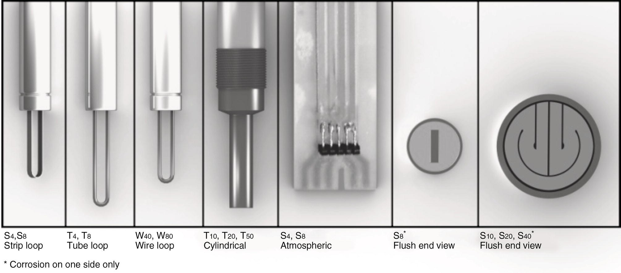
28.2.2 Electrical Resistance Probes
28.2.2.1 ER Probes Determine Corrosion Rates by Measuring Changes in Resistance
 the probe’s rated element thickness, which in this example would be 5 mils (127 μm) corrosion. Thus, if the corrosive environment was 5 mpy (127 μm/year), the probe could theoretically be used for up to 1 year. However, if the corrosion rate was 20 mpy (508 μm/year), the effective life of the probe would be only 90 days. Consult with the probe manufacturer to obtain the most current data regarding each of their probes, and select the most appropriate probe having a reasonable service life, while at the same time having adequate sensitivity for detecting corrosion.
28.2.2.2 Wire Loop ER Probes
28.2.2.3 Tubular Loop ER Probes
28.2.2.4 Tube or Cylindrical ER Probes
28.2.2.5 Flush Mounted ER Probes
28.2.2.6 High Sensitivity or High-Resolution ER Probes
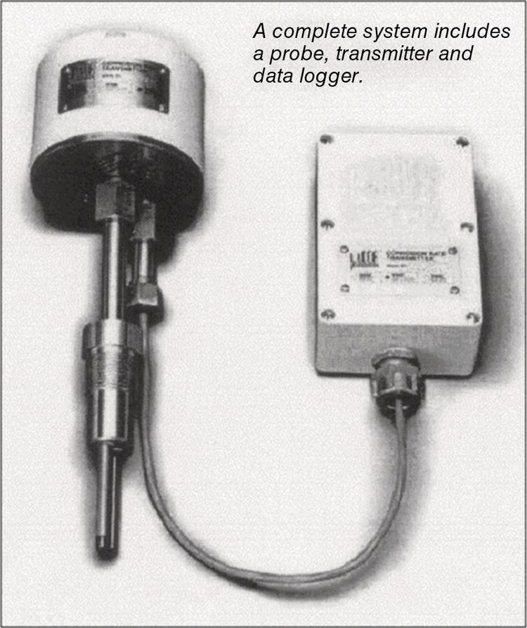
28.2.2.7 Linear Polarization Resistance Probes
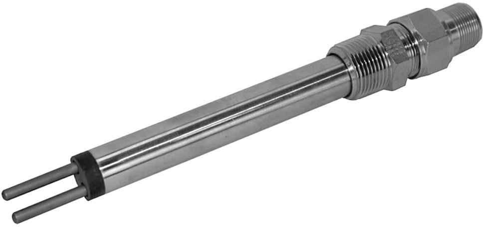
28.3 Placing Corrosion Monitoring Coupons or Electronic Probes Within Pipelines
28.3.1 Placement of the Corrosion Monitoring Point on a Pipeline
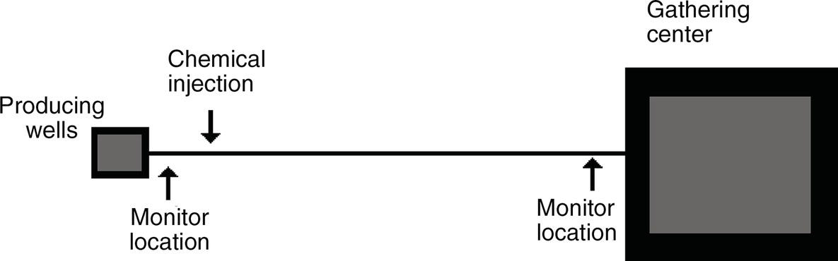
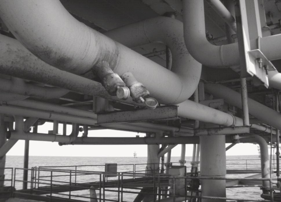
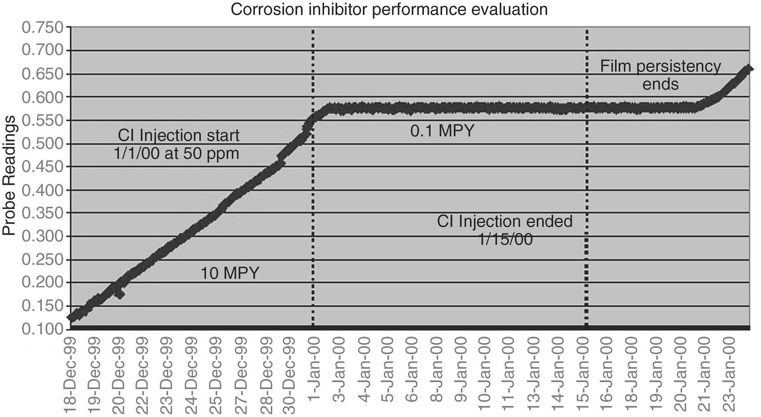
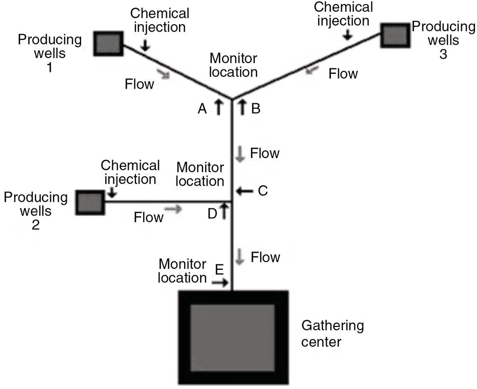
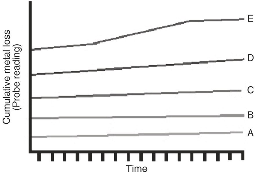
28.3.2 Orientation of the Corrosion Monitoring Coupons or Electronic Probes Within a Pipeline
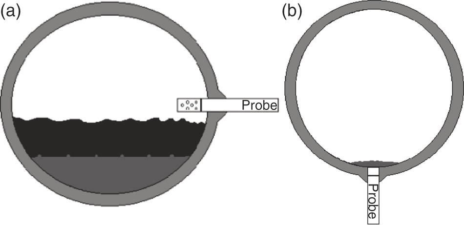
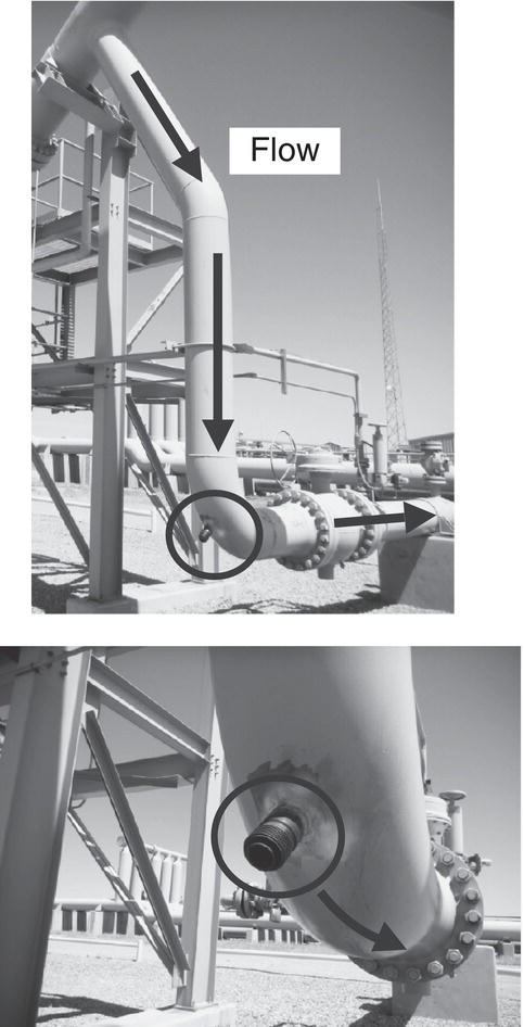
28.4 Monitoring Results “Drive” Chemical Treatment and Maintenance Pigging Programs
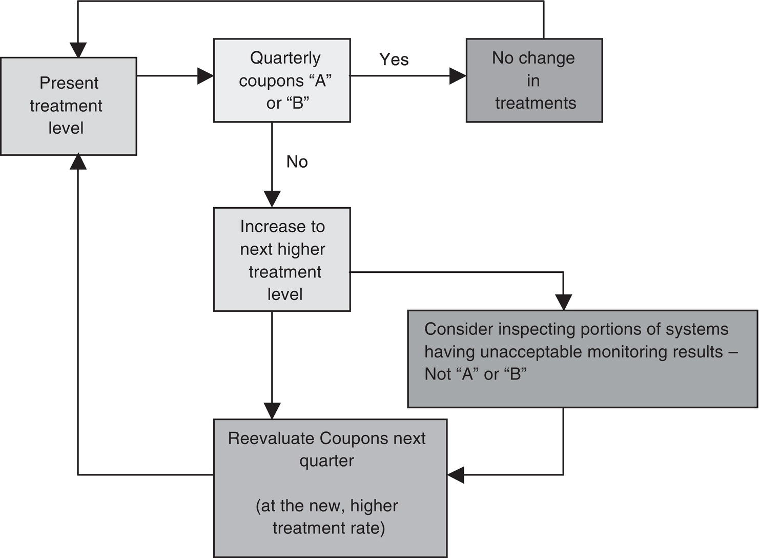
Monitoring or Inspection Technique
Time to Detect and Confirm 10 mpy (254 μm/year) Corrosion Rate
MFL
2–3 years
Ultrasonic or radiography
1–2 years
Metal coupon
30–60 days
Most sensitive wire loop ER probe
4 days
28.5 Relative Sensitivities of NDT Versus Internal Corrosion Monitoring Techniques
28.5.1 Precision of UT, RT, or MFL Nondestructive Inspection Techniques
28.5.2 Typical Exposure Periods for Coupons or ER Probes to Detect Active Corrosion
28.5.3 Relative Time for Coupons, ER Probes, or Inspection Techniques to Detect Active Corrosion
28.6 Seek Consistency Between Internal Corrosion Monitoring and NDT Results—Confirm Trends
28.7 Look for Consistency: Fluid Sample Analysis Should Complement and Verify Monitoring Results
28.7.1 Identify Potential Sample Collection Points Nearby and on Same Production Stream
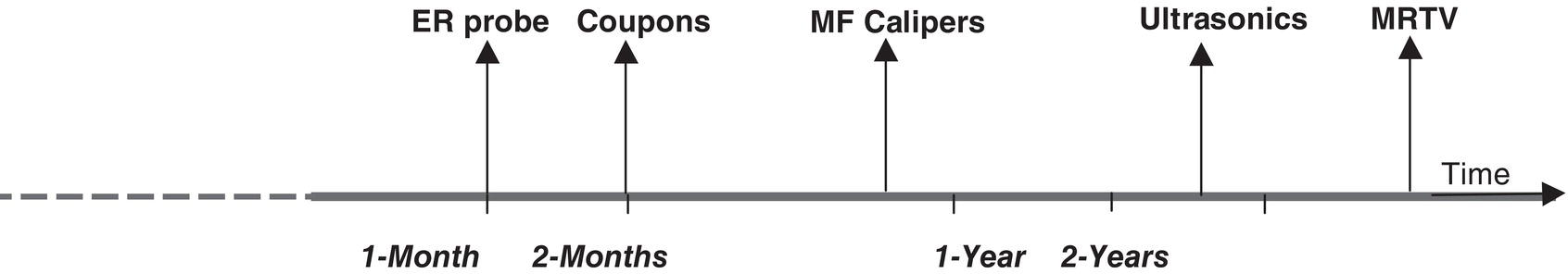
28.7.2 Sample Analysis Variables Commonly Assessed
28.8 Summary
28.9 Definitions of Corrosion Monitoring Terms
References
Notes
Internal Corrosion Monitoring Using Coupons and ER Probes
(28.1)
(28.1a)

(28.2)