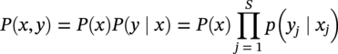
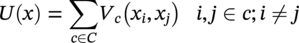
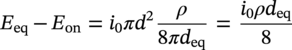
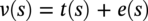
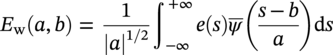
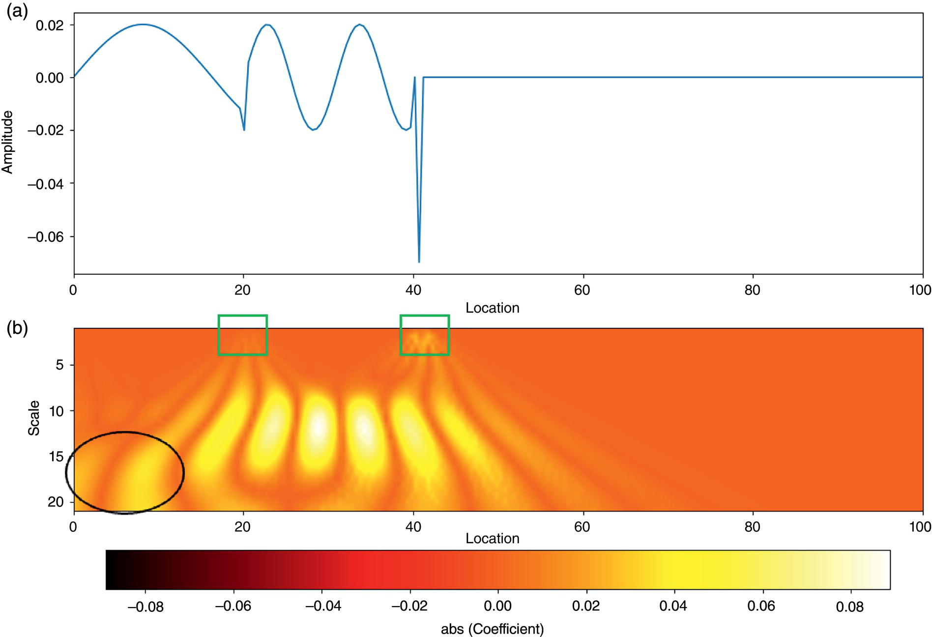
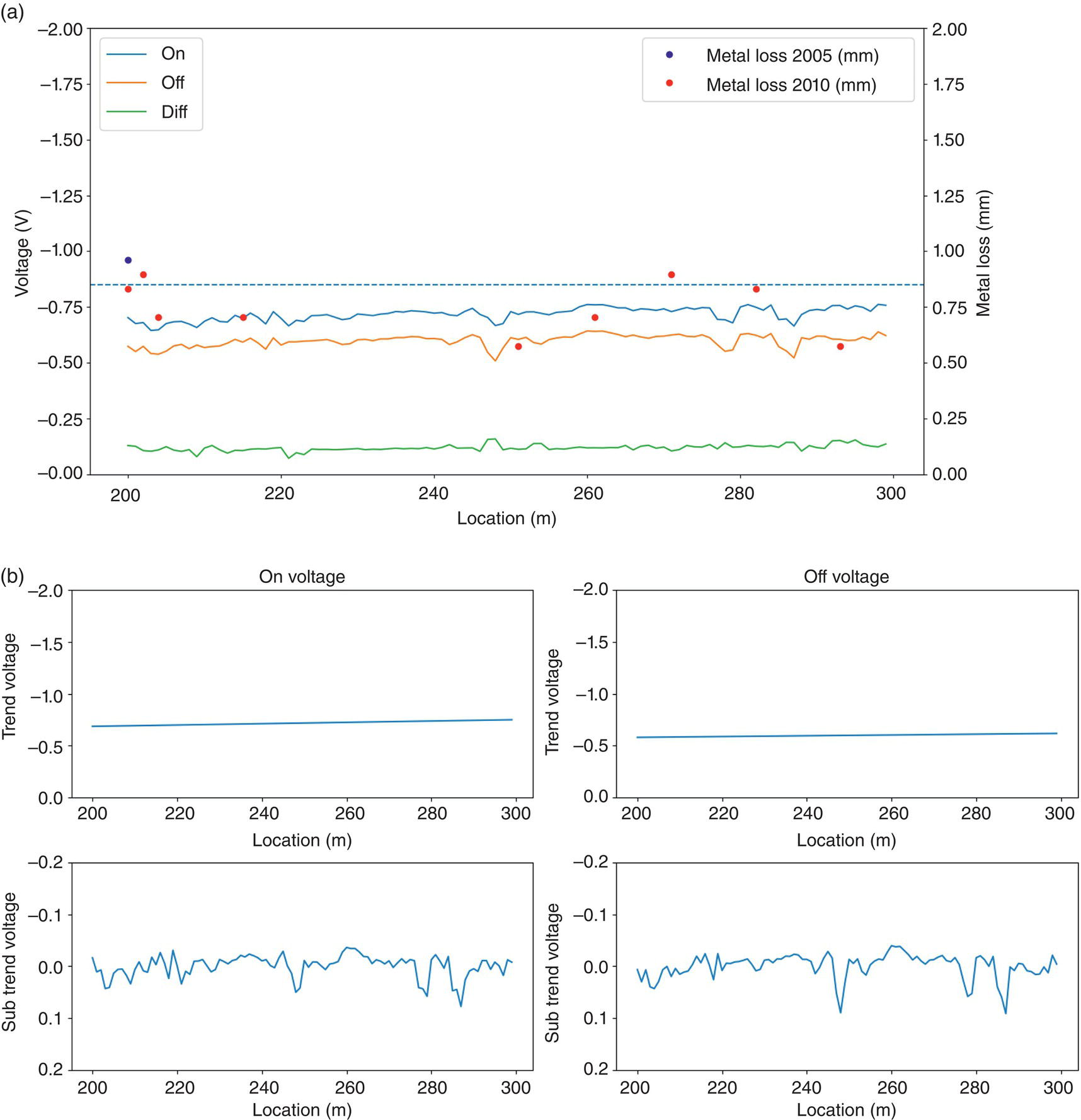
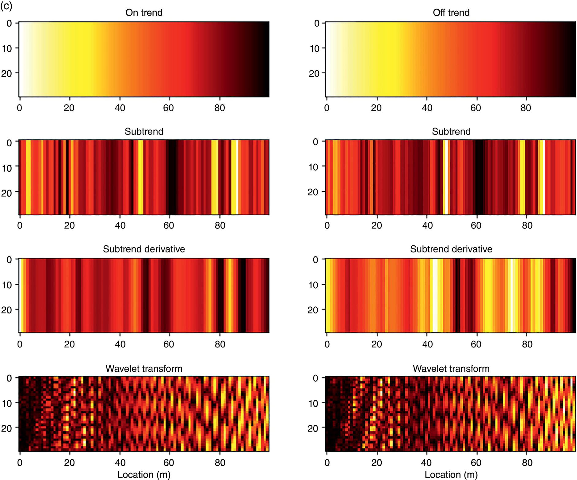
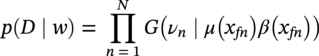
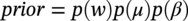
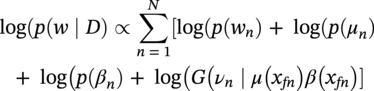
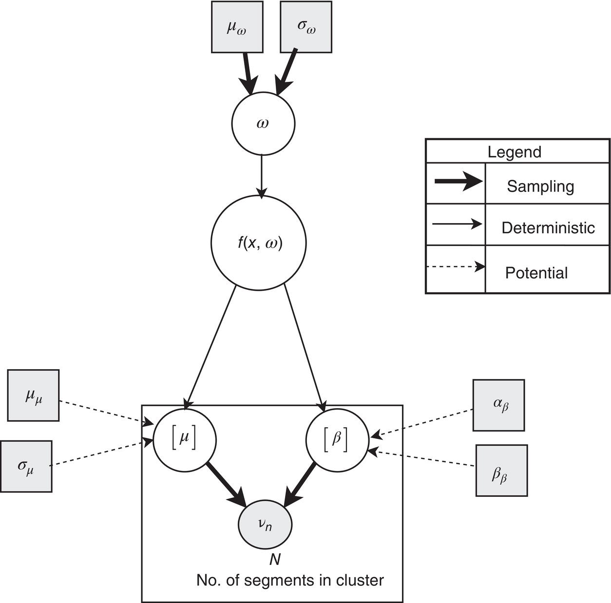
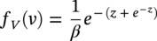
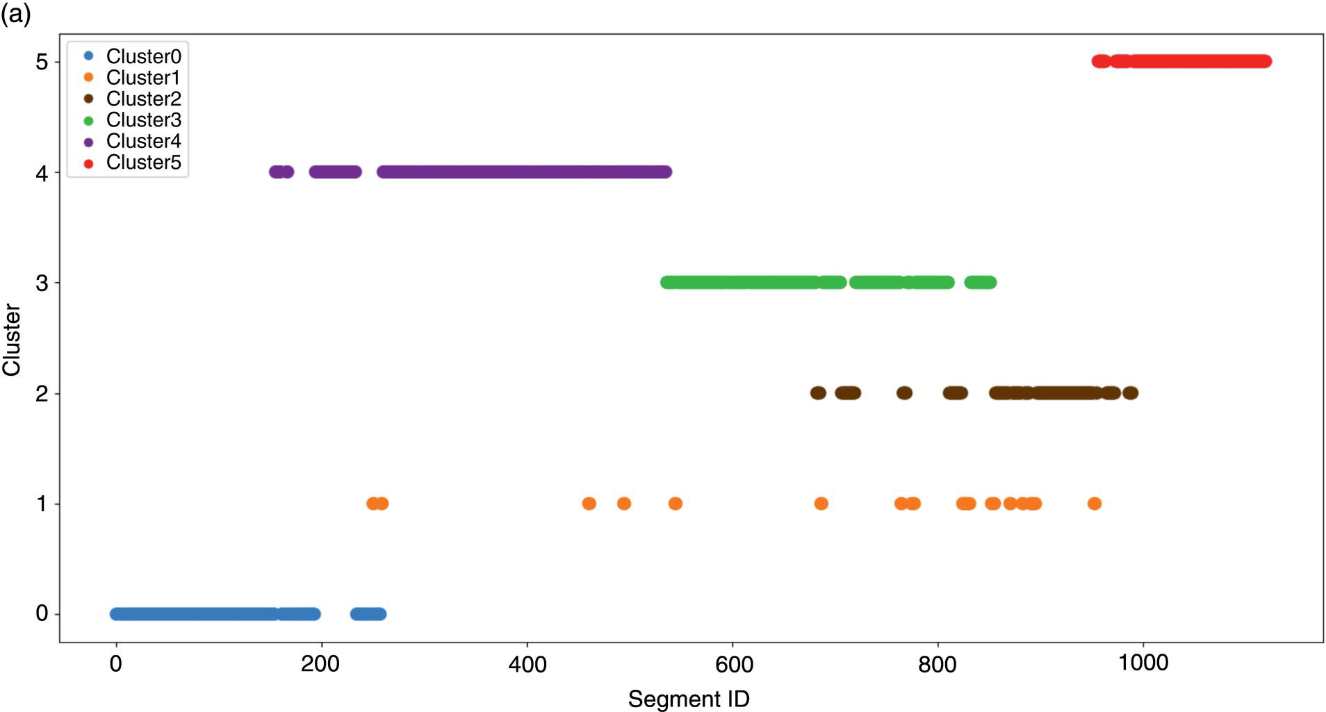
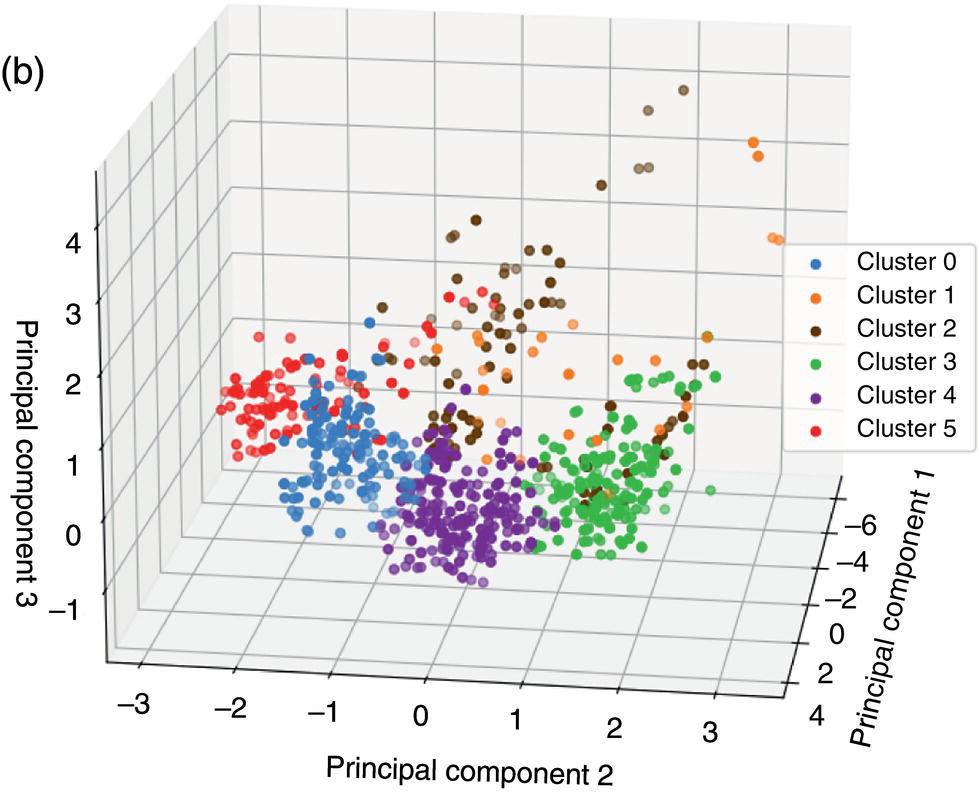
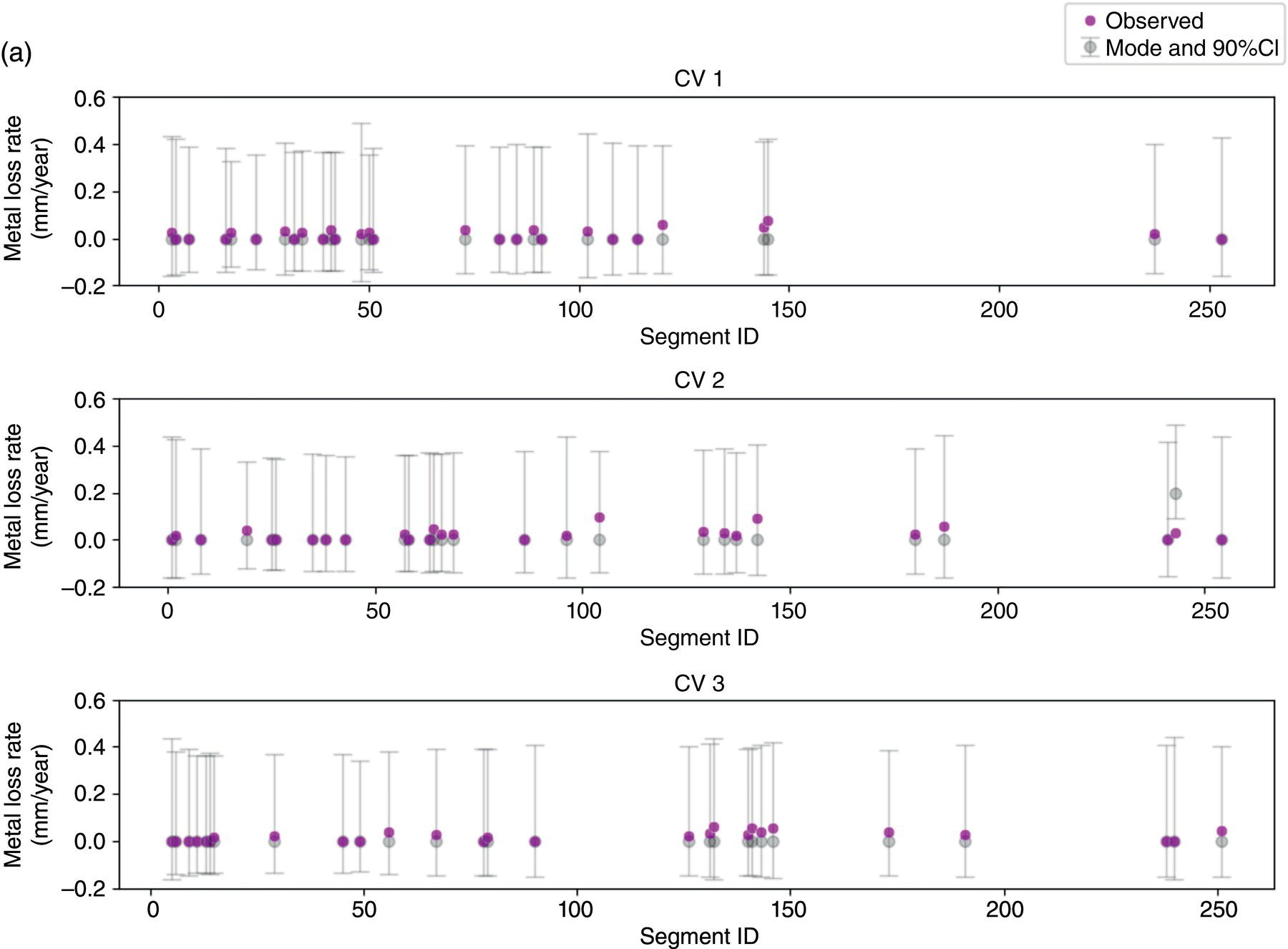
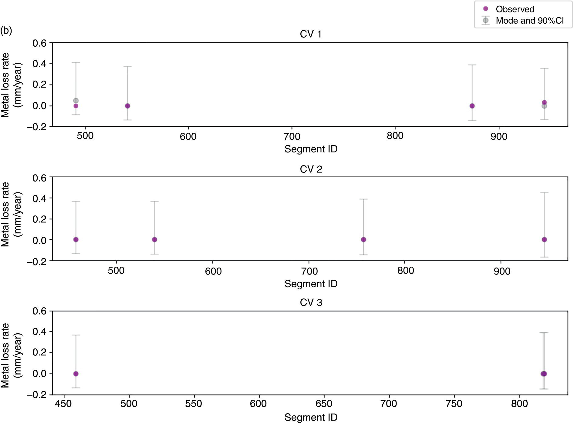
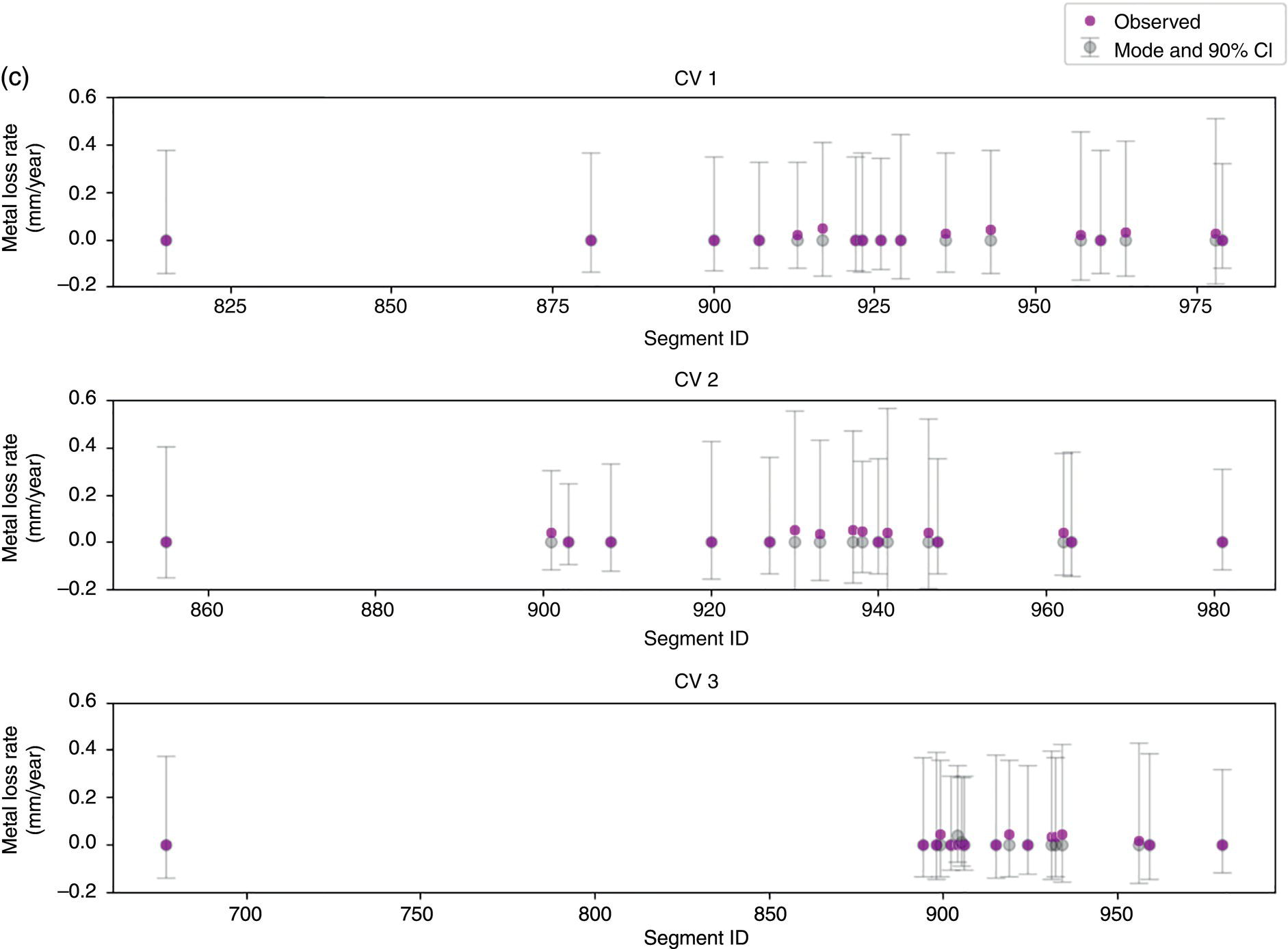
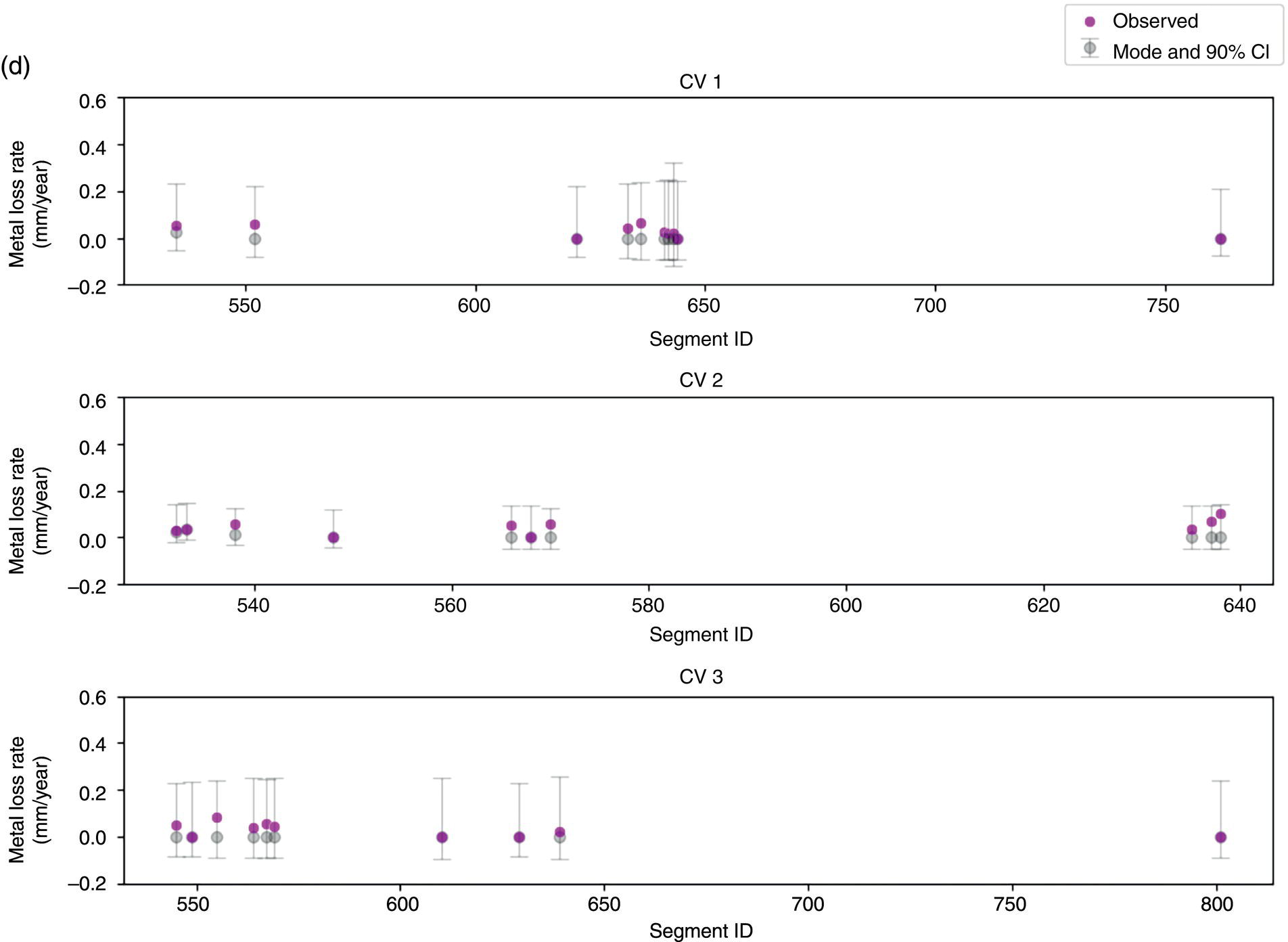
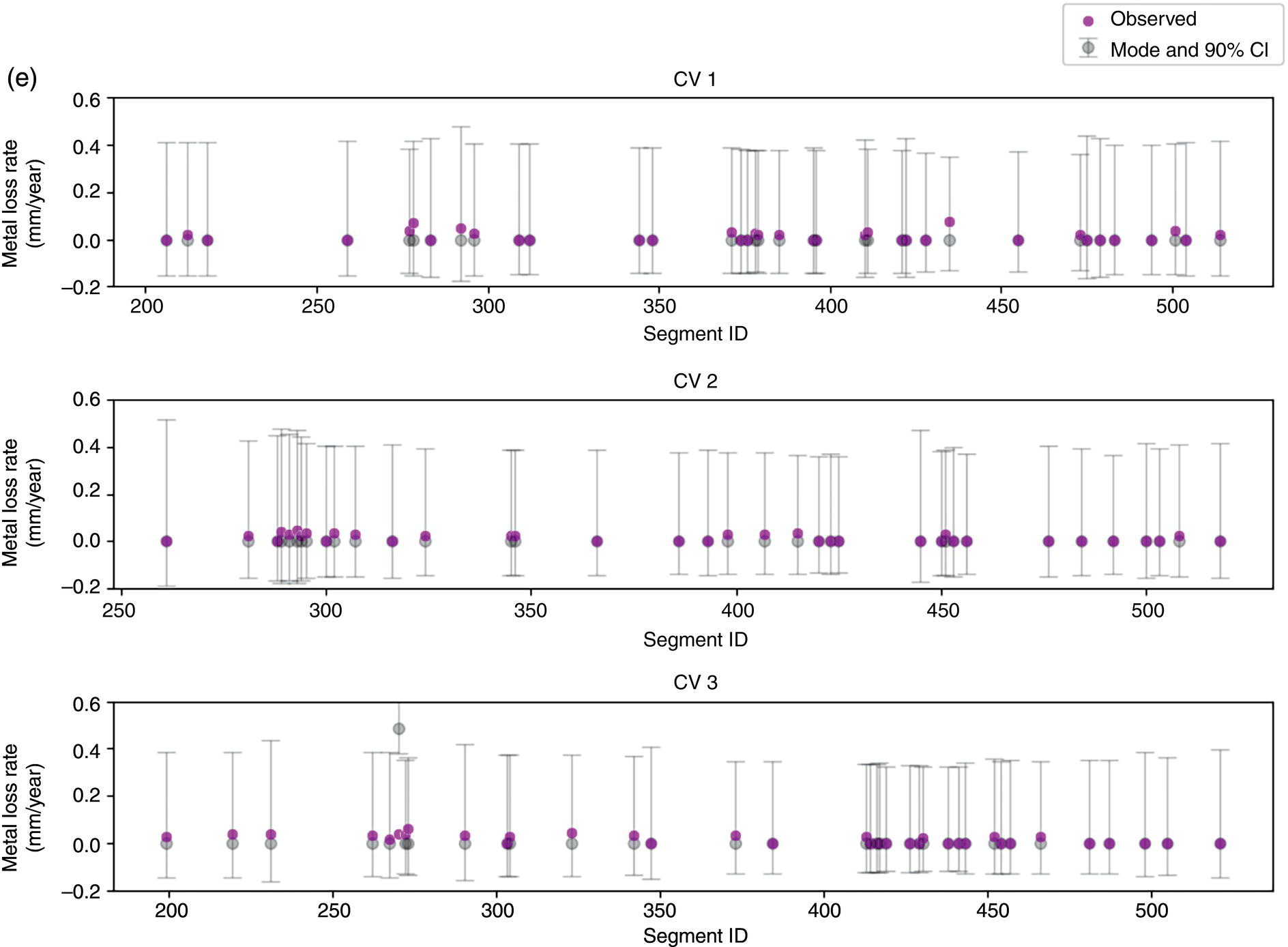
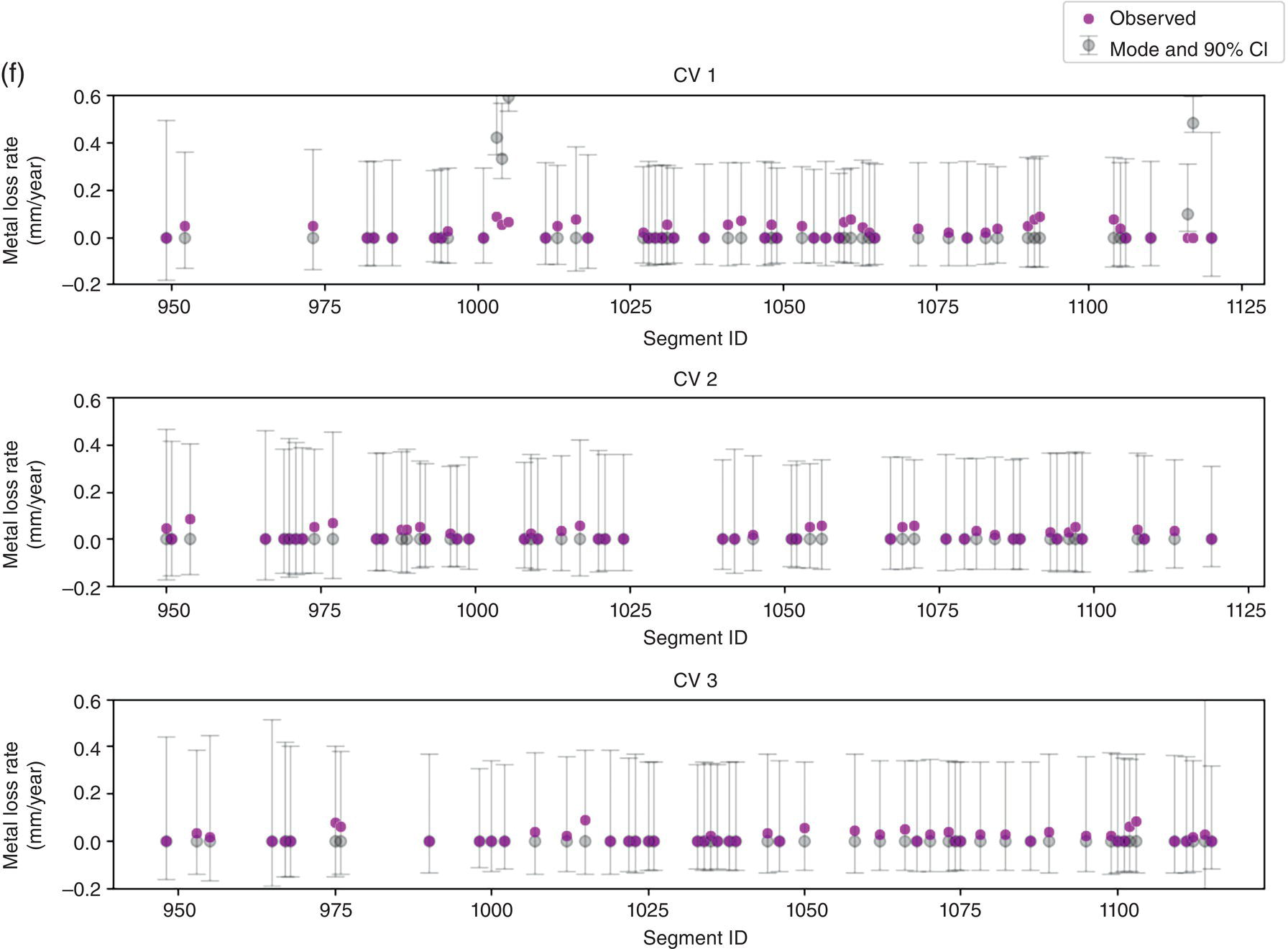
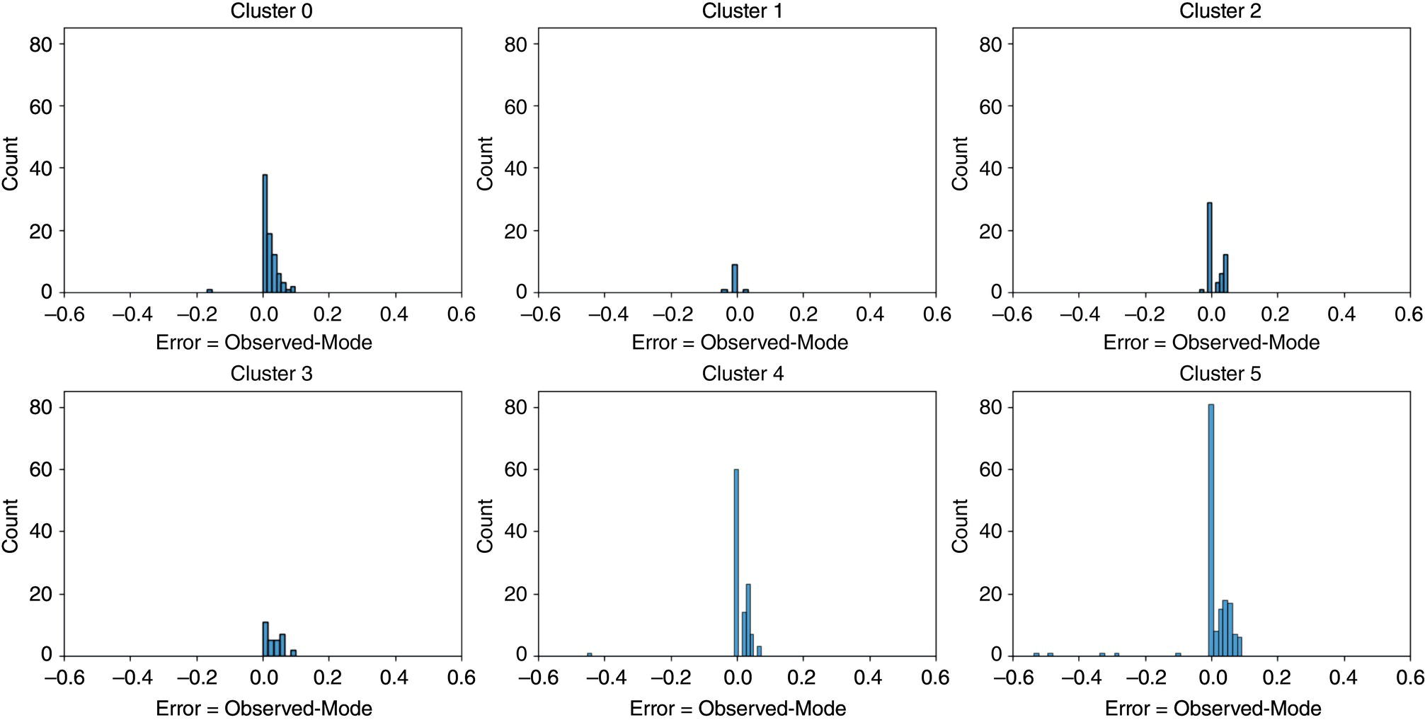
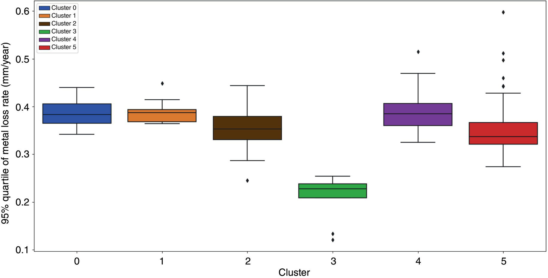
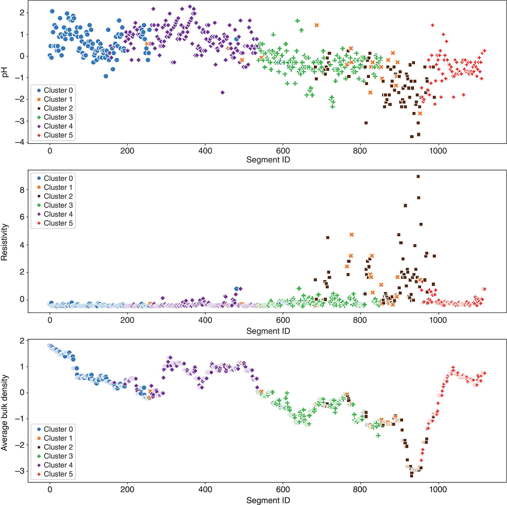
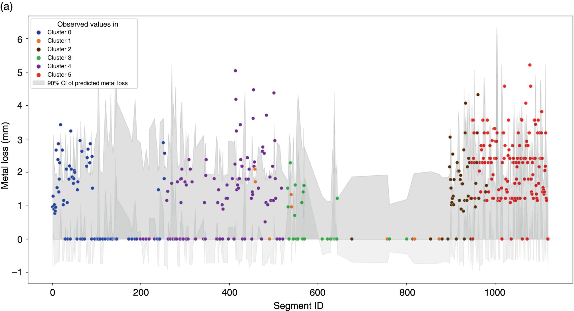
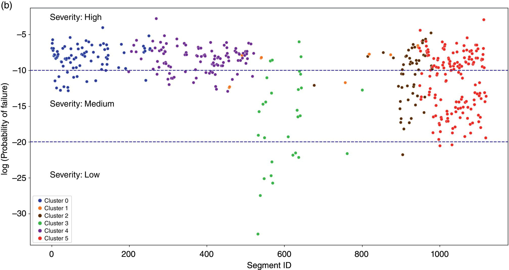
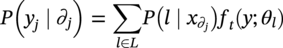
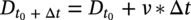
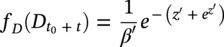
Hui Wang1 Homero Castaneda2 and Sreelakshmi Sreeharan3 1Department of Civil and Environmental Engineering, University of Dayton, Dayton, OH, USA 2Materials Science and Engineering Department National Corrosion and Materials Reliability Laboratory, Texas A&M University, College Station, TX, USA 3Department of Electrical and Computer Engineering, University of Dayton, Dayton, OH, USA The failure of pipelines due to corrosion has devasting effects on both society and environment. Safe and cost-effective operation of buried pipelines can only be achieved through constant monitoring and informed decision making based on knowledge and accumulated data. Currently, the protection of underground pipelines is done by implementing integrity management programs [1]. These include the preassessment of pipeline in which data on pipeline physical characteristics are collected including indirect inspections to identify possible regions of defects and severity, direct assessment of pipeline structures and postassessment or analysis of collected data to determine possible root causes and remaining pipeline life. Even though there are well-established methods and industry practices like Close Interval Potential Survey (CIPS) and Direct Current Voltage Gradient [2] designed to indirectly assess the state of pipeline corrosion, the systematic and formal data analysis approaches for pipeline external corrosion assessment are rather underdeveloped. Pipelines are typically protected by a combination of protective coatings and cathodic protection (CP). The objective of CP systems is to cathodically polarize the pipeline within a potential range of 850–1200 mVCSE. The increase in pH at the metal surface due to the cathodic reduction reaction helps to protect pipeline structures from further corrosion. According to NACE1 current standard practice, pipelines are divided into zones [1] and indirect inspection methods are selected based on soil conditions during preassessment, but soil corrosivity variations are not considered during indirect inspection data analysis. Literature shows that the minimum CP required locally for the passivation of steel is found to be dependent on the type of surrounding soil, bedding conditions, stray currents, disbonded coating and presence of microbial activity [3–5]. All these factors contribute to the change of pH in the pipeline surroundings, which in turn affect the CP required to protect the pipeline. He et al. [6] studied the effectiveness of CP using buried steel specimens in different soil samples in situ and attenuation of CP potential. Hence, the CP level required to protect pipeline structures along the pipeline right-of-way (ROW) is not uniform and depends on the local environment. CIPS is an indirect inspection method generally used to evaluate the criteria for adequate CP and to identify local deficiencies in the system. CIPS is conducted by measuring the potential of a buried pipeline at a given location known as pipe-to-soil potential at regular intervals along the pipeline. Kowalski [7] gives a detailed description of the technique and industrial practice for the interpretation of CIPS data. Designing and applying a varying CP potential along the ROW is difficult and not cost-effective. Instead, analyzing the inspection data considering the soil heterogeneity could help better locate defected regions. Hence, using knowledge- and data-driven approaches to group similar pipeline segments together in terms of soil environments and developing mitigation approaches for each group of segments potentially can be a better strategy. Amaya-Gómez et al. [8] proposed a dynamic segmentation method to divide the pipeline based on soil properties to identify preliminary critical segments. Wang et al. developed a framework using a clustering technique to divide pipeline structures based on soil heterogeneity and studied the evolution of corrosion propagation in each pipeline segment. In this chapter, we introduce the use of the clustering technique. It considers both statistical similarity and spatial variation of soil corrosivity along the pipeline ROW [9]. Anomalies in underground pipelines could be caused by corrosion (external, internal, and stress), structural/welding events, or equipment failure. Voltage measured by CIPS reflects disturbed variations due to any of these anomalies. Signals obtained from CIPS measurements are nonstationary. Hence, a suitable method that can retain spatial and frequency information is preferred. Wavelet transform splits the signal into multiple components with different scales and then shifts the locations of the wavelet window for generating a spectrogram [10]. The spectrogram obtained is a two-dimensional representation of the spectrum of frequencies from the one-dimensional CIPS voltage signals as it varies with location along a pipeline segment. These spectrograms can be used to distinguish different types of signals produced from the pipeline segments. Since the mechanism of CP in a real soil environment is complex, the CIPS data is inherently uncertain. A Bayesian approach capable of quantifying this uncertainty is required, and hence, the Bayesian Convolutional Neural Network (BCNN) model is adopted to make use of the features extracted from the CIPS voltage profile, to predict the maximum empirical metal loss of each segment. This chapter is organized as follows: In Section 50.3, we discuss the model framework and necessary theory. In Section 50.4, we illustrate the applications results of the proposed method to a pipeline system, and in Section 50.5, we discuss the possible limitations, and in Section 50.6, we conclude this chapter. The objective of this work is to develop a framework to determine the severity of pipeline segments by combining CIPS and in-line inspection (ILI) data and by considering soil heterogeneity. Analysis of CIPS data begins with the clustering of pipeline segments using unsupervised learning based on soil heterogeneity. CIPS voltage profiles of segments in each cluster are used to extract 2D input features used in BCNN to predict the maximum empirical metal loss for each segment. The results obtained from BCNN are used to determine probability of failure of segments due to external corrosion. Figure 50.1 shows the workflow for the proposed model framework. In this work, we begin with an approach to cluster pipeline segments into different groups by considering a larger feature space. As pointed out by Melchers in the review paper [11], soil particle size determines the size of localized corrosion, and this dependency is limited to the availability of oxygen to the corrosion regions. Hence, while studying soil impact on pipeline corrosion, it is important to consider soil’s physical properties along with the topology of the surrounding environment. Therefore, in this study, a feature space consisting of physical soil properties like the bulk density of soil, percentage sand content, clay content, coarse fragment, and silt content; large-scale environmental features like land elevation, yearly mean precipitation, and average normalized difference vegetation index (NDVI); soil electrochemical properties from site samples like pH, different ion concentrations, half-cell potential, and resistivity was used. By conducting the wrapper method of feature selection, ten soil features—soil resistivity, soil pH, soil redox potential (Eh), Figure 50.1 Workflow for model framework. In this chapter, Hidden Markov Random Field (HMRF) is used to find hidden patterns in each data when a response variable is not explicitly given, which in this work is the corrosion levels at each pipeline segment due to the soil environment. Though the level of soil corrosivity varies along the ROW, nearby soil environment should have similar level of corrosivity. HMRF is a combination of Markov Random Field (MRF) theory and finite mixture model which can characterize the spatial variations of soil data along with spatial constraints. Let S = 1, 2, 3, 4 …, s denote the sequential ID of segments from the beginning to the end of the pipeline. The state space (indicating the corrosivity level of each segment) of a segment, j ∈ S is given as Xj = {xj ∣ xj ∈ L} hence the configuration space of the entire pipeline can be defined as The main properties of HMRF can be described as follows: Based on these properties the joint probability of clustering configuration and the corresponding observed soil properties is given as, The probability distribution function of a certain configuration of segments based on Gibbs models has the form [13]. where Z is a normalization constant, T is the temperature, and U is the Gibbs 120 energy function given as, where c is a clique corresponding to two consecutive pipeline segments j and j + 1 in the one-dimensional Markov random field and C is the set of all such cliques within S. Vc is the clique potential dependent on the local configuration of c. The random field p(x) is an ordinary one-dimensional Markov random field having a neighborhood system defined as ∂j = {s ∣ s − j ∣ ≤ λ, s ≠ j} and integer λ is named as the order that characterizes the range of spatial constraint. The marginal probability of the observed soil properties yj given the neighboring soil states x∂j for a given pipeline segment j is described as, where θl = μl, ∑l represents the model parameters of the lth Gaussian mixture density. Equation (50.5) is the HMRF–Finite Gaussian Mixture (HMRF–FGM) model used in the unsupervised clustering of pipeline segments. The optimal number of clusters that best fit the given dataset has high intra-similarities within each group and low inter-similarities between groups within the feature space. For model-based clustering wherein the expectation maximization (EM) algorithm is used to find the maximum mixture likelihood for a Gaussian mixture model, Bayesian Information Criterion (BIC) can be used to find the number of clusters. BIC is defined as: where loglike(x, θ) is the maximized log-likelihood, M is the number of independent parameters to be estimated, and n is the number of data points. According to literature, selecting the number of components where BIC will not significantly increase is appropriate [14]. Traditionally buried pipelines are protected from external corrosion by a combination of CP and coating. The aim of CP is to polarize the pipeline below its equilibrium potential (Eeq), below which corrosion is acceptably low. In the case of a steel pipeline at normal conditions, this voltage is −0.85 V CSE (copper sulfate reference electrode). The efficiency of CP on a pipeline system is verified using CIPS. CIPS is conducted by measuring the potential of a buried pipeline at a given location known as pipe to soil potential at regular intervals along the pipeline. This voltage is measured between the pipeline and a reference electrode. Two measurements are made at each location, when CP is working known as on potential and off potential which is the instantaneous potential measured when CP is switched off. The off potential approximates a potential that does not contain the ohmic drop contribution. The potential measured at each pipe location on the surface is given as, where η is the excess voltage above Eeq and IR is the ohmic voltage drop. Accordingly, the off potential is, According to literature [15, 16] the on-potential can be used to estimate coating defect size when Eon measured on the vertical line of the defect given as: where ρ is the environmental resistivity in ohm-m, and deq is the maximum equivalent defect diameter, i.e., the diameter of a hypothetical circular defect whose area is equal to the total defect area summed up within one square meter of the coated surface. Taking Eeq = −0.85 V CSE and protection current density of bare steel in soil i0 = 0.15 A/m2, Hence, the CIPS on voltage is directly dependent on soil resistivity, equivalent defect size, and intensity of corrosion current. CIPS ON/OFF measurements along a segment give the variation of voltage due to anomalies and surrounding soil properties. Each voltage is measured as a function of location(s) which gives the voltage profile for each segment of the pipeline denoted as v(s). According to our hypothesis, the voltage profile v(s) of each segment can be assumed to be a function of the underlying trend t(s) due to soil or macro electrochemical dynamics among segments and sub-trend e(s) due to anomalies on the segment given as, The sub-trend voltage contains information on defects/anomalies as these are the variations caused locally due to the defects. The aim of this study is to differentiate each anomaly and hence determine the severity of each pipeline segment. Hence, the key in this data analysis is finding the descriptors that best differentiate each segment’s sub-trend profiles. Fourier Transform (FT) is a powerful tool that looks at the signal in the frequency domain, but FT works best if the input signal is stationary. Moreover, FT captures the global frequency information and in defect detection local information is important. An alternate approach that retains the spatial and frequency information is the wavelet transformation (WT) [17]. In WT, the signal is convolved with the “mother” wavelet, and then the “mother” wavelet is scaled to accommodate lower and higher frequencies. Wavelet analysis has the advantage of adaptive resolution with various wavelets that can reveal aspects of data such as breakdown points, discontinuities, and self-similarity, and hence can be applied to problems like signal analysis in the case of audio and image compression, smoothing, and image denoising, detection of gravitational waves, earthquake analysis, etc. CIPS sub-trend voltage profile can be considered another example. Applying it to the CIPS sub-trend sequential data is promising since both spatial and frequency-related information can be extracted simultaneously from the one-dimensional data sequence, and it can provide us with richer information regarding the anomalies. The continuous wavelet transforms (CWTs) sum up the signal over the entire spatial domain multiplied by the wavelet function. The CWT coefficients give the correlation between the mother wavelet and the signal component at the given spatial frequency and location. If there is a major feature at the given location and frequency, the CWT coefficients will be significant. CWT of the sub-trend signal e(s) is the convolution of e(s) with the scaled and shifted version of “mother” wavelet ψ(s). The CWT of e(s) is a function of two variables a > 0 and b defined as, where ψ* is the complex conjugate of the “mother” wavelet, a is the scaling parameter that measures the degree of compression, and b is the shift parameter that determines the spatial location of the wavelet. For high frequencies, compressed wavelets are employed to improve spatial localization, and at low frequencies, longer wavelets are used. To understand how fluctuations caused by anomalies are reflected in a CWT spectrogram consider synthetic data of oscillatory signals with two frequencies varying with location with voltage drops of the same width. Figure 50.2 shows such a signal and its corresponding CWT. The lower frequency signal is seen as contours at high scale marked in black oval and the prominent signal with higher correlation is seen at higher frequency. The voltage drops are seen at very high frequencies with similar shapes but different correlation strengths corresponding to variations in amplitude. Each of the signals present in the composite signal is decomposed at three scales of varying intensities. Field CIPS signals are such composite signals, hence, CWT can better decompose the signal to differentiate each anomaly. Figure 50.2 (a) Synthetic signal and its corresponding (b) continuous wavelet transform. The CWT decomposes the 1D CIPS sub-trend into a 2D spectrogram containing the frequency and positional information of each anomaly. The signal frequency changes when there is a change in signal profile, and this change in frequencies is dependent on the defect locations in the segment. Hence, a WT gives information of signal frequencies based on the location which is useful in better understanding the e(s) signal. Each segment has ON/OFF voltage profiles, and the voltage profile consists of a trend and sub-trend. Along with trend, sub-trend of ON/OFF voltages, the derivative of sub-trend, and CWT of the sub-trend are determined. The derivative gives information on slope variation in voltage from defect to nondefect or vice versa. CWT gives 2D information on signal frequency along the segment at different frequency bands in terms of correlation coefficients. Figure 50.3a shows the CIPS profile for a segment, and Figure 50.3b shows the corresponding trend (t(s)) and sub-trend (e(s)) profiles. Figure 50.3b shows ON/OFF image features extracted for the segment ON/OFF trends, sub-trends, the derivative of sub-trend, and wavelet transform of sub-trend. Since the data is 2D, convolutional neural networks (CNNs) are ideal for data analysis. In the conventional CNN training process, network parameters are updated by learning from labeled examples which give a single set of values for each given input. This network fails to quantify the uncertainty in the predictions. In the Bayesian approach, probability distributions can be integrated into the neural network using the Bayes theorem. This now becomes a probabilistic model capable of quantifying the posterior uncertainty. In the given problem, we need to predict the maximum empirical metal loss for each segment (corrosion rate) ν from input vectors xf. The conditional distribution p(ν|xf) is a Gumbel distribution with an xf-dependent mu μ and beta β given by the output of the CNN model. The prior distribution over the weights w of each layer is Gaussian of the form, Figure 50.3 (a) CIPS voltage profiles (b) trend (t(s)) and sub-trend (e(s)) profile for a typical segment (c) extracted features from the voltage profiles. For a dataset of N inputs xf1, xf2, xf3, …, xfN, and corresponding observations D = {ν1, ν2, ν3, …, νN}, the likelihood function is given as [16], To regularize the model further, priors for the Gumbel distribution parameters need to be defined. In the Bayesian framework, prior distributions express one’s belief/knowledge of parameters before having observations. For each model parameter, identical, less informative priors are applied to observations from all soil clusters. We can make assumptions that the parameters of the Gumbel are themselves generated by some prior distributions. Gumbel distribution is assumed to have a normally distributed mu parameter μ and gamma-distributed beta parameter β > 0. Hence, the BCNN has w, μ, and β parameters and prior is defined as, and the posterior distribution is defined as, The BCNN model can be better visualized using the Probabilistic Graph Models (PGMs) with plate notation, where the plates indicate repetition in the generative process. Each node in the graph is associated with a random variable, and the edges encode relations between the random variables. The rectangular boxes indicate a repetitive process of the subgraph inside, and the corner number indicates the number of repetitions of the subgraph. The variable f(X) corresponds to the entire BCNN. Figure 50.4 shows the probabilistic model of the BCNN. Figure 50.4 Plate notation of BCNN. An important application of the proposed model is its ability to predict the uncertainty in corrosion rate and to determine the probability of failure in each pipeline segment. The rate of an external corrosion process is highly dependent on the exposure time, and it has been well documented that the corrosion rate of freshly exposed steel decreases with time following an initial period of rapid corrosion. Hence, for pipeline segments with exposure time greater than 20 years it is assumed to have reached steady state corrosion rate [18]. Based on this assumption, the external corrosion depth at the time ∆t in the future where ν is the corrosion rate of the segment whose probability density function (PDF) is a Gumbel distribution with parameters μ and β, determined using the BCNN model. The PDF of ν is given as, where Applying Equation (50.19) and simplifying we get, where, The probability that all pipe walls at corrosion sites survive at any time t is given as, where w is the pipe wall thickness and Dmax(t) is the maximum corrosion depth at the time t = t0 + Δt. Hence, the probability of failure is given by, As an illustration, the model framework is applied to a real-world underground pipeline system. The pipeline in the study was manufactured using API 5L X52 grade steel and installed in 1969, but certain segments have been replaced over the years after multiple services. The general property information about the pipeline installation, segment replacement, manufacturing material, pipeline segment dimensions, resistance, etc., is well recorded. It has a total length of 110 km, diameter of 457.2 mm, and with a minimum wall thickness of 6.4 mm. The pipeline is divided into 100 m segments for analysis. A soil survey conducted in 2012 provided soil electrochemical properties (pH, different ion concentrations, half-cell potential, and resistivity). The physical properties (bulk density of soil, percentage sand content, clay content, coarse fragment content, and silt content) and large-scale environmental features (elevation, yearly mean precipitation, and average NDVI) were obtained from open source satellite databases. This information was used to conduct the cluster analysis to identify the heterogeneity of soil corrosivity. CIPS was used as part of a proactive survey of pipeline conditions to indirectly assess pipeline conditions. The CIPS data are collected for approximately every 1 m over the underground pipeline. The data consist of ON voltage taken with CP on, OFF voltage taken when CP was instantaneously off, and information regarding obstructions, water bodies, presence of high voltage lines, etc. These CIPS data were used to extract input features for the BCNN, as explained in the model framework. Data from two inline inspections conducted in 2005 and 2010 were available. The inspections were conducted using magnetic flow leakage (MFL) in 2005 and ultrasonic testing (UT) in 2010. The inspection data consist of location, pigging date, type, and size information of defects. The date of installation from general pipeline data and the pigging date from ILI are used to determine the years of service of each pipeline segment. Old segments of years of service greater than 30 are taken for analysis. Defect depth from ILI 2005 is temporarily normalized by dividing it by years of service and the temporarily normalized maximum depth or the maximum empirical metal loss in each segment used as the target for training the BCNN model. A set of 11 features was selected from the entire feature space using wrapper feature selection which were further dimensionally reduced to seven PCs using PCA. Based on these PCs, the optimal number of clusters was determined using the BIC criteria as six. Unsupervised HMRF–FGM cluster analysis was conducted, and Figure 50.5a shows the results of cluster analysis, and Figure 50.5b shows the scatter plot of three PCs in six clusters, which shows the dispersion and sparsity of each cluster. Based on the soil states of each pipeline segment obtained from the clustering analysis, the CIPS data are labeled along the pipeline right-of-way. CIPS data for each segment along the ROW is grouped into six clusters based on pipeline surrounding properties and features for determining the distribution of maximum empirical metal loss extracted from each segment. The BCNN model for each cluster is validated using three-fold cross-validation (CV). Figure 50.6 shows the 90% credible interval (CI) of metal loss rate distribution for each cross-validated test data. Each different cluster has a different maximum corrosion rate, and almost all observed values are found to be within the predicted Gumbel distribution of the corresponding segment. To further understand the performance of the model, Figure 50.7 shows the estimated error between observed data and the model of the Gumbel distribution corresponding to the maximum probable value. For most of the clusters, the error lies close to zero indicating that the estimated value is the most probable metal loss rate of each segment. Even though the ILI data show no defect for some segments, the segments need not be clean; instead it can be assumed to have shallow defects that cannot be detected by the ILI instrument. Hence, a good model should be able to predict a low or ignorable level of empirical corrosion rate for clean segments. Figure 50.8 shows the box plot of the 95th quartile (i.e., the extreme level) metal loss rate of clean segments (according to ILI) in each cluster. Clusters 2 and 5 show spread in predicted rate which on further analysis could be due to the fluctuating soil properties as shown in Figure 50.9. Since the pipeline environment itself is unstable, the prediction of metal loss rate is also unstable for clean segments. Other clusters show a small spread in predicted metal loss rate indicating similar soil conditions within a cluster. Figure 50.5 (a) Clustering results (b) Scatter plot of three principal components in six clusters. Based on the metal corrosion rate distribution estimated for each cluster, the metal loss after five years is predicted, which can be compared with the ILI data obtained in 2010. The results of predicted metal loss 90% CI along with observed metal loss obtained from ILI in 2010 is shown in Figure 50.10a. Furthermore, the severity levels of each cluster based on the probability of failure calculations using Equations (50.22–50.24) for each segment are estimated and shown in Figure 50.10b. Clusters 0 and 4 have more segments in the high severity range, and Cluster 3 has segments in the low severity range. Therefore, based on the distribution of estimated corrosion rate in each segment, the future corrosion depth and thereby severity of each segment can be estimated using the proposed framework. Figure 50.6 Test data cross-validation results for (a) Cluster 0, (b) Cluster 1, (c) Cluster 2, (d) Cluster 3, (e) Cluster 4, and (f) Cluster 5. Figure 50.7 Error estimation of metal loss rate in each cluster. Figure 50.8 Predicted extreme (95% quantile value) metal loss rate for clean segments (identified from inline inspection). Figure 50.9 Cluster groups of soil features: elevation, resistivity, and average soil bulk density along the pipeline right-of-way. This chapter presents the concepts of knowledge- and data-driven external corrosion modeling and implementations using the recently developed unsupervised and supervised machine learning algorithms. Some explorations in using data-driven approaches for pipeline external corrosion management have been conducted, and the preliminary results have been reported. Since this is an emerging field with an active research community, more and more new approaches will be reported in the future. Having observed recent strong and rapid improvements in AI and its use in engineering applications, it is anticipated that more sophisticated models will be developed and applied in pipeline external corrosion-related applications for efficient and effective risk management. Figure 50.10 (a) 90%CI of predicted metal loss with true values in each cluster (b) Probability of failure on log scale for segments in each cluster along the ROW.
50
Knowledge- and Data-Driven External Corrosion Modeling in Pipelines
50.1 Introduction
50.2 Background
50.3 Model Framework and Theory
50.3.1 Workflow for CIPS Data Analysis
50.3.2 Review of Clustering Analysis for Identifying Heterogeneity of Soil Corrosivity
 concentration, Cl− concentration,
  concentration, and
  concentration, land elevation, yearly mean precipitation and soil bulk density are selected. Moreover, to incorporate the variability of soil aeration conditions along the pipeline, ROW difference and mean soil bulk density around the pipeline environment are considered. A total number of eleven properties from the feature space is used for cluster analysis. A dimension reduction to the selected eleven features was done using principal component analysis (PCA) [12], reducing the feature space to seven principal components (PCs). PCA is a technique for reducing the dimensionality of large datasets, increasing interpretability but at the same time minimizing information loss. It does so by creating new uncorrelated variables that successively maximize variance.
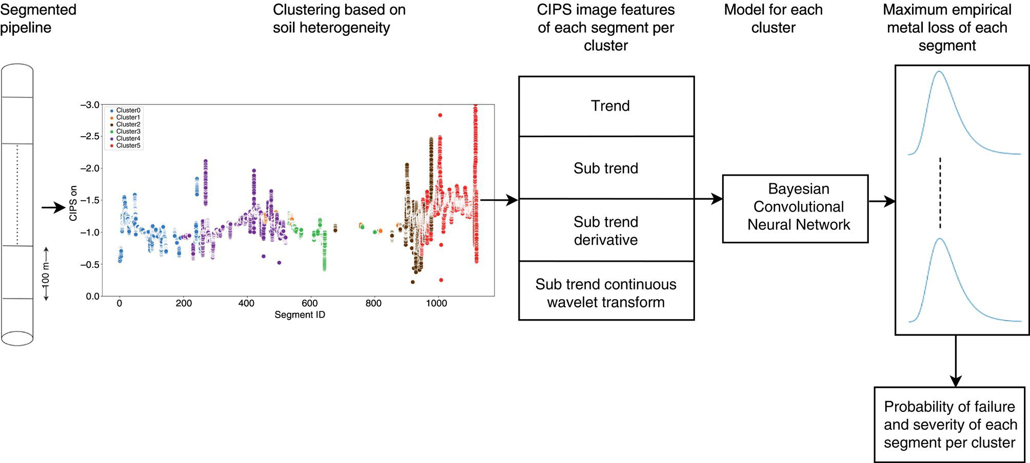
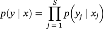
 . The state values of all the sites x = (x1, x2, x3 … xs) are a configuration in the product space X, and the configuration defined on S is considered as a random field given as p(x). If yj denotes the PCs of segment j then the feature space random field p(y) is the product space denoted as
  , where Yj = {yj|yj ∈ Rd} and y = (y1, y2, y3 … ys). Rd is the d-dimensional feature space framed by the most significant PCs.
 ).
).


50.3.3 CIPS and Wavelet Transform


50.3.4 Bayesian Convolutional Neural Network


50.3.5 Reliability Analysis
 , based on the current corrosion depth
  can be determined as:
 , μ and β are the location and scale parameters of the Gumbel distribution. Therefore, the distribution of corrosion depth after ∆t years is given as,
 hence the parameters of the distribution of predicted corrosion depth
  are
are  and β′ = β∆t.

50.4 Model Application
50.4.1 General Information
50.4.2 Clustering Results
50.4.3 BCNN Results
50.5 Limitations of the Approach
50.6 Conclusion
References
Note
Knowledge- and Data-Driven External Corrosion Modeling in Pipelines
(50.2)
(50.3)
(50.4)
(50.6)
(50.7)
(50.8)
(50.9)
(50.10)
(50.11)
(50.12)
(50.13)
(50.14)
(50.15)
(50.16)
(50.17)
(50.18)
(50.20)
(50.21)
(50.23)
(50.24)