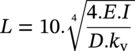
Andy Young ROSEN UK Ltd, Newcastle upon Tyne, UK The surface of the earth is affected by a wide range of natural processes. The three main natural processes that shape the land surface are: There is an additional significant process: the influence that humans have on the landscape, ranging from agricultural practices to the development of urban areas and transportation infrastructure. Tectonic activity is another significant factor, which results in the development of mountains and basins over the longer term (millions of years), but it also causes rapid changes following seismic events, such as, the occurrence of landslides, the displacement of geological faults and liquefaction hazards. When the route for a new pipeline is selected, it is standard practice to consider all environmental threats that may affect the pipeline. Geological, geomorphological, geotechnical, river, and seismic specialists are normally involved in the identification and characterization of these threats, and the route is adjusted to avoid significant hazards as necessary. It may not be possible to avoid specific threats, such as the crossing of active geological faults or some landslides due to other constraints, and in these cases, mitigation is applied to reduce the loading on the pipeline so it can survive the design loading event. Alternatively, in the case of landslides, measures are taken to stabilize the hazard. Other options may involve the use of strain-based design. Geohazard threats can also arise during the service life of the pipeline. Despite detailed studies of the right-of-way at design, extreme or unexpected events leading to ground movement loads may occur. In some cases, the hazard is subtle and may have existed prior to construction but was not identified. In contrast to design, rerouting around hazards that occur or are identified during operation is a major decision with high-cost implications. This decision requires strong justification. Establishing a reliable estimate of the current integrity of the pipeline and how this changes with future movement is essential to avoid wasted investment or inadvertent damage and failure. Pipelines that cross areas of high geohazard susceptibility can be designed to withstand the higher load demands that could arise. This will normally involve strain-based design with particular reference to the properties of the girth welds [1, 2]. Pipelines that were not designed for strain limits, which include the significant majority of onshore lines [3], may have unknown properties or are not covered by the applicability range for existing girth weld strain models. This inevitably forces the selection of a more conservative strain capacity limit or significant extra work to identify relevant weld properties. A process is required to manage geohazards during the service life of the pipeline, and it should involve the main elements of identification, evaluation, and mitigation. In simple terms, operators need a geohazard management plan to answer two main questions: The answers to these questions will determine whether intervention and protection measures are required. The subject of geohazards and geohazard management is very broad and there is a significant volume of published work. This chapter is mainly focused on the integrity management of operating pipelines and how they can be protected from adverse loads. Consequently, it concentrates on the identification and evaluation of unplanned loading on pipelines from geohazards rather than the geohazard itself or on route planning activities. It is intended mainly for pipeline engineers with a responsibility or interest in this area. A general introduction to geohazards is provided, however, this is a brief description with selected references to more comprehensive sources. The significance of loading is generally judged against the structural load capacity of the pipeline. Performance limits are discussed in detail elsewhere (in other chapters); however, it is important to recognize that the load capacity can be impaired by the presence of geometric anomalies or other defects that need to be considered in the threat management. Although geohazards normally represent the most onerous form of loading on pipelines, other load sources can also be significant. For example, these include civil engineering activities as well as loads generated by the installation of the pipeline. The effect of these load sources on pipeline integrity is also considered within this chapter, although the generic term of geohazard loads is used frequently throughout. The chapter is split into the following main sections: Section 47.2 covers a brief introduction to the primary types of geohazards that can affect pipelines. Section 47.3 notes some key regulations and guidance on geohazards for pipelines, including management procedures. Section 47.4 outlines the geohazard management process with emphasis on the protection of pipelines. Section 47.5 describes hazard identification, including the use of bending strain from in-line inspection (ILI). Section 47.6 lays out how identified hazards can be evaluated, including the use of structural calculations. Section 47.7 briefly describes the options for hazard mitigation and monitoring. The general guidance in this chapter applies to buried pipeline sections and does not cover associated installations. Geohazards are surface processes or ground conditions that can result in failure or damage to pipelines or require significant cost to mitigate their effects. Typically, this involves some ground movement event on the pipeline right-of-way. The relative displacement between the stable and unstable blocks of ground can generate forces in buried pipelines that cross the affected zone. This chapter mainly considers the identification and evaluation of geohazards or loads that are currently affecting pipelines, and therefore, are an immediate integrity concern. However, geohazard threats may also be present on or adjacent to the right-of-way but have not affected the pipeline yet. These hazards also need to be addressed within a geohazard management plan for existing pipelines. There are many publications that provide a detailed description of geohazards (e.g., [4–11]), including some references that address pipeline integrity issues. The following sections provide a brief introduction to the main types of hazards, primarily for those unfamiliar with the subject area. Landslide hazards are widely recognized as one of the most significant threats to pipelines by operators (Figure 47.1) and involve the downslope movement of soils and rocks due to gravity. These are associated with the steeper slopes in mountainous or hilly terrain but can also develop on shallow slopes with gradients of less than 10%. There are a number of different types of landslides [8] but slides and lateral spreads are normally the most hazardous to buried steel pipelines. Lateral spreads are triggered by earthquakes and can occur on slope gradients that are less than 3%. The cause of landslides can be complex, but the most common factors are changes in groundwater or moisture in the slope predominantly due to precipitation, and also seismic ground shaking from earthquakes. The severity of the threat from landslides to pipelines is governed by a number of factors: Correct identification of the presence and nature of the landslide is the important first step in hazard management; this process is covered in Section 47.5. This step will determine whether the landslide is an immediate integrity concern that should be investigated further. Figure 47.1 Pipeline crossing the head area of an active landslide. (With permission of ROSEN (UK) Limited.) Where an active landslide is identified that may affect the pipeline, the size, direction of movement, and soil characteristics need to be established, as these control the load transferred to the pipeline. The speed of the landslide movement influences the time available to assess the problem and take protective actions. This is linked to the type of landslide and its environment. A number of studies [12, 13] have examined the historical occurrence of pipeline failures from landslides. When locations of pipeline failures are classified according to landform, higher failure rates are indicated in mountainous regions, as is expected; this is illustrated for Europe in Figure 47.2. The failure rate is 40 times higher in mountains than across all terrain (labeled “all” in Figure 47.2). The failure rate for old pipelines in South America (Andes) is significantly higher than for new pipelines. Sweeney et al. [12] point out that the more recent failure rate is reduced due to modern practices of increasing effort to identify and avoid hazards in combination with higher pipeline strength due to improved welding. Factors of improved construction practices on the right-of-way and particularly the control of drainage have also reduced the number of failures. Future trends are uncertain because of the increasing effects of climate change on slope instability due to more extreme rainfall events and major erosion problems [15–19]. Geological faults are natural near planar breaks in the rock below the ground surface that can extend for considerable distances and depths (i.e., several km or 10s of km). Active faults undergo periodic movement due to the sudden release of forces that have built up within the earth. This is particularly true at the margins of tectonic plates. The earth’s surface is made up of 15 large tectonic plates that move under the motion of convection currents within the underlying mantle, and the collision at the junction of the plates generates immense forces within the earth. Figure 47.2 Pipeline failure frequencies due to landslide mainly in mountainous areas Figure 47.3 Location of sag ponds on the major North Anatolian Fault in Turkey. (With permission of ROSEN (UK) Limited.) The movement on the fault plane is the cause of earthquakes generating seismic waves. The fault movement on larger faults can extend to the surface, and the ground displacement is a significant hazard to any pipeline that crosses the plane. The location and activity state of geological faults can be defined; however, it is not possible to predict with any degree of accuracy when movement will take place because of the complexity of factors that control the build-up of force and strain in the rocks on either side of the fault. These forces are strongly influenced by the structure of the rock, involving subsidiary faults and fractures, as well as the distribution of previous earthquakes, which includes many smaller seismic events that are more frequent than the larger damaging ones. The hazards of geological faults should be addressed at design by identifying the presence and activity state of any faults that are crossed on the pipeline route. For active faults, which are generally accepted as denoting the occurrence of movement within the Holocene geological period (i.e., the last 11,000 years), mitigation measures are applied. This is undertaken because it is not possible to state with any certainty that movement will not occur within the service life of the pipe. The North Anatolian Fault in Turkey (Figure 47.3) is one of the most active faults in Europe. Extending over a distance of 1500 km, it is crossed by a number of pipelines (see, e.g. [20]). A total of 12 earthquakes with a moment magnitude (MW) of 6.5 or higher occurred on the fault plane between 1939 and 1999, and movements in excess of 6 m have been reported. However, no incidents of movements causing the failure of major oil and gas transmission pipelines have been reported to date. A range of geological factors need to be considered when quantifying the hazard from active faults [21]. The pipeline engineering aspects during operation will typically involve structural analysis of the effects of fault movement on the pipeline (see Section 47.6.4). This takes into account the interpreted components of horizontal and vertical movement on the fault plane and the orientation of the pipeline at the crossing of the fault plane. The fault movement components are linked to the nature of the fault plane and to whether this is a normal, reverse, or strike-slip fault. Both the North Anatolian Fault in Turkey and the San Andreas Fault in California are examples of dominantly strike-slip faults. In addition to the movement magnitude, the number of distinct shear planes on which movement takes place needs to be established, together with the fault zone width over which ground deformation occurs. Estimates of fault movement may be based on paleoseismic data (evidence of historical earthquake movement). This would typically involve excavation of trenches across the fault location and a detailed examination of the nature and age of soil and rock exposed within the trench walls. The offset of natural surface features, such as stream channels due to movement along the fault plane will also reveal the rate of fault movement. Figure 47.4 Relationship between surface rupture length and maximum fault displacement. (Adapted from Ref. [22].) An alternative approach is to use statistical data on measured fault movements from previous earthquakes correlated against the length of the fault plane rupture at the surface. A well-known data source published by Wells and Coppersmith [22] is based on measurements at 95 faults involving a combination of all three main types of fault geometry (Figure 47.4). The most practical protection option for operational pipelines is to reduce the load transfer from a future fault movement event onto the pipeline. This can be achieved by installing low stiffness backfills around the pipeline, cutting the trench walls to shallow angles or reducing the ground cover in the region of the fault crossing. These need to be validated by structural analysis. If uncertainty remains over the ability of the pipeline to withstand the predicted future loading, a more detailed assessment should be undertaken, including investigation of the girth weld properties in the areas of high loading. Revised calculations using the girth weld properties may be sufficient to confirm adequate load capacity, but in the event the loads are still predicted to exceed limits, replacement may be required. Practical design guidance is provided in [23–25]. Liquefaction is the temporary change from a solid to a liquid state and occurs during earthquakes that affect saturated granular soils. The seismic shaking causes a transient increase in the pressure of water within the pores of the soil, which reduces the strength of the soil so it flows like a fluid. Ground hazards due to liquefaction that affect pipelines include buoyancy, settlement, and lateral spreading, which is also described as a form of landsliding [8]. Of these, lateral spreading provides the highest threat to buried pipelines. Liquefaction commonly occurs in sediments within flat, low-lying areas, such as flood plains, shorelines, and estuaries. This is because the soils in these areas are generally recent deposits from the Holocene geological period (the last 11,000 years) and are, therefore, more likely to be loosely consolidated. Plus, groundwater levels are generally high in these environments. Assessment normally involves reviewing the pipeline route to establish locations that could be prone to liquefaction. Locations that may be prone to liquefaction on pipeline routes are normally based on identifying the presence of susceptible soil deposits and sufficiently high ground motion levels from earthquakes. For example, this could be a peak ground acceleration (PGA) that exceeds 0.1 g, where g is the gravitational constant within a specified return period. The likelihood of exceeding a specific PGA within a specific return period, typically 50 years, can be predicted by probabilistic seismic hazard assessments (PSHAs). For locations where liquefaction movement can occur, the magnitude of lateral spread movement can be estimated for two environments: [26] Locations where the potential for liquefaction is identified to be moderate or high should be subjected to increased scrutiny. First, this involves field visits by appropriate geotechnical experts to confirm the nature of the environment and any historical evidence of ground disturbance. The second activity involves testing the strength of the soils to identify the presence of potential liquefaction layers. This will typically involve standard or cone penetration testing (SPT or CPT) to map the properties and extent of the subsurface layers. Assessment will involve structural analysis based on the estimated ground movement profile. Protection options for existing pipelines are more difficult than when the assessments are included in the design. Pipe lowering to below the liquefiable layer may be one option. Reducing the load transfer onto the pipeline at the margins of the potential movement zone may also be possible. These options are likely to require justification using structural analysis. The acceptable pipeline performance limits can be maximized by determining the properties of the girth welds to derive an improved estimate of the tensile strain capacity. Ultimately, however, if the threat is considered high and mitigation options are limited, rerouting may be the only option. Detailed guidance on the management of pipelines affected by seismic hazards is available in [23–25, 27, 28]. A common cause of natural ground subsidence is the solution of limestone, including chalks (see Figures 47.5 and 47.6), which can create fissures, gullies, and cave systems within limestone bedrock. The subsequent collapse of the void generates a sinkhole at the surface. These features are typically between 2 and 50 m wide but can reach 100 m [30]. Figure 47.5 Surface depression associated with the development of a sinkhole in an area underlain by chalk in the U.K. (With permission of ROSEN (UK) Limited.) Figure 47.6 Development of a sinkhole in chalk adjacent to a high-pressure pipeline in the U.K. [29]. (With permission of ROSEN (UK) Limited.) The distinct landscape created by rock solution and collapse is described as karst. Salt (halite) and gypsum are also examples of soluble rock. The main threat to operational pipelines is the potential loss of bedding support to the pipeline leading to a spanning section. Subsidence of natural ground can also occur in soils. Examples include: Loading from natural ground subsidence in soils is less of a threat to buried pipelines than karst terrain because the magnitude of subsidence is normally smaller, so spanning is less likely. However, the loading from differential movements can be significant in the boundary areas, particularly if there are abrupt changes in geology or groundwater conditions or in support conditions, for example, adjacent to cased road crossings. Settlement in soils can present a threat to above-ground installations, particularly due to the loss of function of the pipe supports. This may result in pipework that exceeds elastic performance limits and, therefore, requires remediation activity. Other sources of subsidence linked to human activities are covered in Section 47.2.8. Examples of pipeline loading from ground subsidence are provided in Section 47.5.5. Most long-distance pipeline routes cross river channels at some point, even if these involve ephemeral flow. River crossing areas are particularly active hazard environments, especially during flood events following prolonged or intense rainfall. Current flow can erode the riverbed and the banks of the channel, and in wide, sediment-filled channels, the river may abruptly change course, which is known as avulsion. Erosion and scour of the river channel can result in exposure and spanning of the pipeline (see Figure 47.7), leaving the pipeline vulnerable to additional loads from current flow, vibration or direct impact from water-borne debris and a mobile-riverbed load. Vortex-induced vibration (VIV) is one of the most significant threats and can result in pipeline failure within hours (possibly even less than 1 h) during a flood event. It develops because the pipeline oscillates in the water current due to pressure changes from vortices that are shed from the top and bottom surface of the pipe. Figure 47.7 Spanning pipeline in an estuary crossing. (With permission of ROSEN (UK) Limited.) The factors that control the onset and magnitude of vibration are complex, but the key influences are: Where exposure does occur, it should be addressed to ensure the pipeline remains safe. Pipeline spans need to be of sufficient length for failure to occur. Consequently, determining the maximum allowable span length provides a pragmatic screening process for the severity of the threat. This can be achieved using the River-X software [31]. The example in Figure 47.8 shows the relation between the flow velocity in the river channel and the allowable span length, where VIV develops for a 200 mm nominal diameter pipeline. Acceptability is based on the reduction in fatigue life due to the vibration. Based on the maximum predicted current velocity of 2 m/s from detailed hydrological studies, the calculated allowable span length due to VIV is 21 m. This provides a guide on the level of threat; however, scour can develop rapidly during flood events, and therefore, it is also important to have an understanding of the history of scour behavior as well as the flood characteristics of the river channel. It should be noted that scour holes and channels move, so previously exposed sections can subsequently become infilled. Consequently, some channel sections may exhibit scour during the flood rise but deposition can take place during the ebb period and conceal previously spanning sections. The estimated time to failure from fatigue of the girth welds containing workmanship-level defects is provided in Figure 47.9 for the example in Figure 47.8, assuming a span length of 25 m has developed, which means that the span is longer than the acceptable span at the current flow rate of 2 m/s. The fatigue life reduces rapidly at the onset of vibration, which occurs at velocities of approximately 1.3 m/s in this example. At a flow velocity of 2 m/s, the fatigue life is 75 days, and therefore, failure would probably involve the accumulation of damage from several high-flow events. Figure 47.8 Link between the current velocity and acceptable span length for a 200-mm-diameter pipeline. (With permission of ROSEN (UK) Limited.) Figure 47.9 Predicted fatigue life for a 25 m span at a range of current velocities. (With permission of ROSEN (UK) Limited.) The fatigue life decreases as the current velocity increases, and for the crossing examined in Figure 47.9 failure could occur within 1 day should a flow velocity approaching 5 m/s be possible in the channel. A comprehensive review of pipeline spanning and fatigue problems including operational experiences in North America is provided in [32, 33]. Pipelines at river crossings should be designed to prevent exposure by ensuring they are buried with a sufficient depth of cover so that they lie below the maximum predicted scour depth. Installation by horizontal directional drilling will normally be sufficiently deep to avoid these problems. However, many crossings on existing pipelines have been installed by open-cut methods and with little or no account of scour potential. National regulations on pipeline surveillance may set out the requirements for the inspection frequency of river crossings. For example, guidance on the frequency of depth of cover surveys on pipeline crossings in the in the United Kingdom summarized from the standard IGEM/TD/1 [34] is presented in Table 47.1. The frequency depends on both the nature of the crossing and the depth of cover on the pipeline. Table 47.1 Guidance on the Frequency of Surveys (in Years) for River Crossings Source: Summarized from [34]. Measurements of the depth of cover provide reliable evidence regarding the safety of the crossing and whether it is deteriorating. Erosion of riverbanks generates localized instability and slumping. Normally, the pipeline crossing will be sufficiently deep approaching the river so this is not a threat where the channel location is largely stable. However, where lateral channel migration is high, problems of exposure can arise. An example of rapid lateral channel migration that has taken place over 15 years is shown in Figure 47.10. The rate of movement exceeds 2 m/year, and the distance of migration is approximately 3 times the channel width. As a consequence of the erosion, the pipeline section that was previously routed across the flood plain adjacent to the crossing became exposed in the riverbed. Lateral migration also represents a threat to pipelines routed across flood plains parallel to the river channel. Riverbank erosion is a frequent cause of landslides in the adjacent valley slopes because it removes toe support (see Figure 47.11). These hazards can develop rapidly and represent a significant environmental risk, particularly for the consequences of leak or rupture in liquid lines. In addition to the erosion effects from rivers outlined in Section 47.2.4, erosion of soil can cause dramatic changes to the land surface. In most cases, it develops slowly over time, but some intense rainfall events can lead to rapid washout features and gully development (Figure 47.12). Erosion can oversteepen slopes, promote surface water infiltration into the slope soils, change drainage paths, and trigger wider instability on slopes. Soil erosion is rarely the direct cause of pipeline failure, except where large washout occurs on the right-of-way. The typical effects of erosion on the right-of-way will lead to pipeline exposure and spanning. Figure 47.10 Lateral migration of River Caldew in Northern England. (With permission of ROSEN (UK) Limited.) Figure 47.11 Pipeline exposure within slope instability caused by river erosion. (With permission of ROSEN (UK) Limited.) Sheet and rill erosion by wind or water can lead to a general reduction in cover on pipelines across wide areas, particularly in arable land. Although this may ultimately result in exposure, the main threat is the increased risk for third-party damage, for example, due to ploughing activities. The depth of cover on pipelines can be efficiently monitored by the combination of high-resolution inertial measurement unit (IMU) inspection with digital elevation models (DEMs), for example, from light detection and ranging (LiDAR) surveys [35]. This does require accurate surveying of above-ground markers, and these may also be at a reduced spacing compared to standard IMU inspections. Accuracies better than 150 mm can be achieved where the LiDAR survey resolution is 2 m or better. LiDAR surveys for hazard identification are covered in Section 47.5.2. Poor pipeline construction practices and associated post-construction erosion of the pipeline right-of-way in hilly terrain can be a significant issue [36]. Deep erosion gullies promote instability on the slopes and choke drainage courses with sediment. A significant influx of sediment can radically alter the local stability of river systems, leading to changes in the river course and accelerated erosion or scour. In a recent pipeline failure incident investigation, it was established that a large washout had occurred on the right-of-way due to poor drainage practices that had promoted both erosion on the side slopes and water ponding and infiltration on the right-of-way. Spoil excavated from the right-of-way during construction had been tipped onto the side slopes, altering drainage and providing a highly erodible surface. The slopes were slowly oversteepened, ultimately leading to the washout incident after several years of operation. Figure 47.12 Rapid development of a gully, 40 m wide and 5 m deep, in arable farmland in the U.K. (With permission of ROSEN (UK) Limited.) Deforestation during right-of-way construction or for general land use development may also lead to high erosion rates if land stabilization and drainage are not properly implemented. Good construction practices covering the effective control of surface erosion on the pipeline right-of-way and adjacent slopes are essential to maintaining pipeline integrity during service, particularly in hilly terrain with high rainfall. Guidance is available, for example, in references [37, 38]. There are many types of geohazards specific to certain environments, including frost heave and thaw settlements, desert sand dune migration, and volcanic hazards. Information on these is contained in some of the references given in Section 47.2. The climate factors of temperature and precipitation have a significant influence on geomorphological processes and geohazard activity. There are three main climate types: These climate types are subdivided into a number of morphoclimatic zones, which exhibit distinct characteristics and types of geohazards. There is a fourth climate category, which is normally described as azonal and refers to high mountains that can occur anywhere within the three main types of climates. For example, periglacial regions represent one morphoclimatic zone in the polar and tundra climate type. In this region, temperatures lie generally below 0 °C but rise to above 0 °C for short periods in the summer. This causes seasonal thaws of the surface layer of the ground and results in very active mass movements in this layer. Paleoclimates can also influence the presence and nature of geohazards. This is particularly true for relict periglacial terrain where, for example, solifluction deposits formed by the slow mass movement of freeze-thaw activity may contain preexisting shear planes. This can lead to situations where the ground is subsequently destabilized in the current climate regime by ground engineering activities or erosion. The types of morphoclimatic zones and associated types of hazards are described in [39]. A number of civil engineering activities can generate loads that may affect pipelines. These include: Surface loading may include the combined effects of the direct increase in vertical stress on the pipeline and ground settlements due to the consolidation of soft soils that underlie the pipeline. An example of pipeline settlement due to surface loading is illustrated by ILI data and this is shown in Figure 47.33, Section 47.5.5. New pipelines that are routed across areas of landfills may be affected by long-term settlements of the fill, particularly if this contains significant organic matter. Calculations for a recent pipeline construction project where the route crossed a number of former landfill areas indicated that future settlements could potentially lie between 300 and 500 mm. Some loads from civil engineering activities may not represent a threat to pipelines constructed to modern welding standards, such as API 1104 [40] or BS4515 [41]. In older pipelines, however, the presence of poor-quality girth welds will reduce the load capacity, which in turn increases the significance of loads that develop in the pipeline. A common situation for older pipelines is that the quality of the girth welds is unknown; therefore, a cautious approach to performance limits for tensile loads is required (Section 47.6.2). The subsurface extraction of minerals by mining creates a void in the rock strata. Mining by the room-and-pillar method creates a grid of voids separated by support pillars. However, voids may subsequently migrate upwards as the strength of the rock deteriorates over time and the roof strata progressively collapse. This causes crown holes to develop at the surface (Figures 47.13 and 47.14). The likelihood of subsidence tends to be higher for older workings because the mining was generally at shallower, more accessible depths. This can result in the loss of bed support to pipelines that cross the subsidence areas. The problem is compounded for older workings because records of their location are incomplete or do not exist, so subsidence can occur unexpectedly. The assessment of the likelihood of subsidence from historical room-and-pillar mining is mainly based on: Higher-strength rock with a low density of joints (natural rock fractures) and an increased depth of mining has a lower likelihood of subsidence. For historical room-and-pillar mining in the United Kingdom, subsidence at the surface was rarely observed for mine depths more than 10 times the extraction height (seam thickness); however, the actual depth will depend on the mining details and geology. Figure 47.13 Illustration of crown hole formation for historical room-and-pillar mining. (With permission of ROSEN (UK) Limited.) Figure 47.14 Development of a crown hole adjacent to a pipeline route due to historical mining subsidence. (With permission of ROSEN (UK) Limited.) Grouting of voids is sometimes employed during pipeline construction where the hazard cannot be avoided. This is less common during operation due to the cost and uncertainty over subsidence development. The severity of loading threat to the pipeline can be assessed by calculating the maximum tolerable span width that takes account of the soil overburden load on the pipeline. This is then compared to the likelihood of crown hole subsidence developing at the surface that exceeds this width. Occasionally, subsidence from room-and-pillar mining occurs from the progressive collapse of heavily loaded support pillars. This can lead to a larger subsidence area that has similarities to longwall subsidence. Longwall coal mining involves the extraction of large panels typically up to 300 m wide and several km long. This is accompanied by the intentional collapse of the roof strata, creating wide subsidence troughs at the surface. Although subsidence occurs simultaneously with the mining, the effects can also be delayed due to the influence of geological faulting [42]. Longwall mining represents a significant load threat to pipelines that cross the subsidence area, primarily due to the development of ground compression over considerable lengths of the pipeline route, Figures 47.15 and 47.16. Mining in many regions of the world is controlled by licensing and regulation requiring the mine operator to notify affected landowners and land users (including pipeline operators) when mining is planned that could result in subsidence. This should be sufficiently in advance to allow pipeline operators to establish whether the pipeline will be adversely impacted by subsidence so that the pipeline can be protected. Predictions of ground subsidence from longwall mining are typically based on empirical or semi-empirical factors that vary with the geographic region [43]. The working of multiple seams in a subsidence area and complex geological structures, including the presence of faults, influence the reliability of predictions. Subsidence measurements are typically carried out to validate the predictions. Extraction of a single panel can take one to 2 years, and subsidence profiles are typically produced at different stages of extraction to enable refinement and validation of predictions as mining progresses toward the pipeline crossing. This also ensures that the most adverse loading condition on the pipeline is captured. Subsidence predictions including the horizontal components for a pipeline that crosses a 110 m wide panel of coal that is 1.2 m thick and at a depth of 270 m with an intersection angle of 60° (where 90° is perpendicular to the long axis of the panel) are presented in Figure 47.17 [43]. The resulting predicted stress levels in terms of von Mises equivalent stress are shown in Figure 47.18. The allowable stress limit is exceeded primarily due to the influence of axial compression, and therefore further action is required. This could involve more effort in defining the soil restraints, consideration of strain performance limits or measures to reduce the load transfer onto the pipeline, which typically involves temporary excavation during the mining period. For pipelines that have already sustained some ground loading, any stress relief excavation must follow a specific order and direction in order to avoid compressional Euler and local buckling failure, Figure 47.19. Figure 47.15 Illustration of longwall mining subsidence showing areas of ground compression. (With permission of ROSEN (UK) Limited.) Figure 47.16 Axial buckle due to compression from longwall subsidence in the United Kingdom [29]. (With permission of ROSEN (UK) Limited.) Figure 47.17 Example of predicted ground movement components relative to the pipeline for subsidence from a longwall mining panel. (With permission of ROSEN (UK) Limited.) Figure 47.18 Example of predicted von Mises equivalent stresses for subsidence of a longwall mining panel. (With permission of ROSEN (UK) Limited.) Extraction of large volumes of underground fluids, such as water pumping or the production of oil and gas, generates ground settlement. Fluid abstraction results in the reduction of pore pressures within the soil and rock where withdrawal is taking place, which increases the net vertical “effective” stress. The increase in effective stress causes compression and compaction of the geological strata and results in the development of subsidence at the surface. Figure 47.19 Pipeline damage due to excavation in an area of compression due to longwall mining subsidence. (With permission of ROSEN (UK) Limited.) Figure 47.20 Monitored increase in pipeline strain due to settlement following backfilling. (With permission of ROSEN (UK) Limited.) Classic examples of subsidence from oil and gas extraction include the Greater Houston area and Long Beach in California, where settlements of up to 9 m were recorded. For water extraction, Mexico City is a commonly quoted example, with estimated settlements of up to 10 m over the last 100 years and settlement rates of 300 mm/year. Problems of ground compression from fluid abstraction have caused instances of upheaval and local buckling of pipelines at the surface [9]. An example of ground settlement due to water abstraction is illustrated by ILI data and this is shown in Figure 47.34. Construction loads are caused by the fabrication, installation, and backfilling activities for the pipeline as it is buried in the trench during the construction period. They are present in most pipelines to a varying extent and typically involve longitudinal bending. This is because the development of axial force at construction is rare, with the exception of horizontal directional drilling installations and potential minor effects on very steep slopes. Thermal axial force may be generated at the location of tie-ins if there is a significant temperature variation from ambient conditions, typically involving increased temperatures associated with solar gain. Sources of construction strain are considered in relation to IMU inspection surveys in Section 47.5.6. Construction related loads may not develop until sometime after construction. This is typically as a result of time-dependent effects, such as collapse compression or settlement in poorly compacted bedding following initial inundation or submersion by percolating groundwater. An example of this is shown in Figure 47.20, where strains were recorded at three locations on a pipeline following backfilling. In this example, increases in bending strain are observed for up to 6 months following the backfilling stage. Notwithstanding the development of initial loads immediately following burial, the main jumps in strain followed significant rainfall events. The long-term load at the three monitored locations was at least double the initial load. A common situation where increased bending strain occurs is following the backfilling of excavations to inspect or repair pipelines. This is normally linked to poor control or possibly a complete lack of compaction of the bedding below the pipeline during reinstatement, coupled with the pipeline self-weight and the return of the overburden loading onto the pipeline. One example of a 12-in. diameter pipeline is illustrated in Figure 47.21 and involved 200 mm of pipeline settlement leading to the development of high ovality and significant longitudinal bending in the shoulder of the repair excavation. The bending and deformation were detected following a subsequent ILI. A summary of the regulations and guidance on geohazard management is provided in references [11, 14]. Two recent advisory documents from the North American pipeline industry are of particular note: Figure 47.21 Example showing longitudinal bending and the location of significant cross-section deformation (ovality) following the reinstatement of a repair excavation. (With permission of ROSEN (UK) Limited.) This reinforces the requirements to consider external loads and geohazards for natural gas and hazardous liquid lines. It sets out a list of actions to address geohazards where earth movement may affect pipelines. Specific aspects relevant to operational pipelines include: Operators are required to start inspection of affected pipeline sections within 72 h after a geohazard event, such as an earthquake or landslide, providing the area is safe to access. Where adverse loading is identified, operators must take appropriate remedial action to ensure the safe operation of the pipeline. The PHMSA bulletin essentially outlines a geohazard management process for the pipeline from construction to operation. This sets out concerns linked to the failure of girth welds on high-strength pipelines. Global failure strains as low as 0.4% have been reported due to the accumulation of longitudinal strain in the girth weld. This can occur in pipelines that comply with relevant specifications but where the girth weld has a lower strength than the adjacent “high”-strength line pipe. To address the risk, it is advised that project welding procedures and qualification records may need to be reviewed and mechanical testing of the pipe materials may be required to check for weld under-matching and heat-affected-zone softening. While this can be addressed at pipeline design, retrospective actions for operational pipelines are often limited to quantifying a realistic strain capacity for the existing pipeline. An improved estimate of the strain capacity can be developed based on inspection and testing of pipeline girth weld samples. International standard ISO 20074 [47] defines the requirements and content of a geohazard management plan for onshore pipelines. Operators are responsible for the development and implementation of the plan. The standard applies to both new and existing pipelines. Operators are required to provide an explanatory document if they feel a management plan is not necessary for specific pipelines. A geohazards management plan involves three main elements [47]; this applies from design and throughout operation: This chapter is concerned with pipeline operation only, where the focus is on pipeline integrity management rather than design and routing issues. Once a hazard or external load has been identified, the two main objectives are: Figure 47.22 Illustration of a geohazard management process for operational pipelines. (With permission of ROSEN (UK) Limited.) The management plan provides a decision framework to define and schedule actions on appropriate monitoring and mitigation measures to protect the pipeline from the hazard. Some hazards develop so rapidly that a detailed assessment is not feasible and emergency protection or stabilization becomes necessary. The effect of these hazards can be minimized by a robust implementation of geohazard management that recognizes the presence of high-susceptibility areas [48]. An example of a basic geohazard management process for operational pipelines is illustrated in Figure 47.22. The process has strong links with ILI because this provides valuable direct measurement data on whether the pipeline is experiencing loads. It is also possible to interpret the nature of the loading from the ILI data and use it to efficiently assess the integrity of the pipeline. The hazard identification, evaluation, and mitigation activities are covered in more detail in Sections 47.5–47.7. Geohazard threats are typically identified for in-service pipelines by one of the following methods: The integrity management plan for a pipeline should define the inspection and surveillance requirements for pipelines. Minimum surveillance requirements are normally defined by the relevant national pipeline specifications. ILI involving an IMU is a key part of geohazard management because it can detect and measure pipeline displacements that result from applied loads. Audits of the pipeline right-of-way by geohazard experts may be warranted where: When considering the content of a geohazard management plan, it is important to weigh up the perceived cost savings (or false economies) of not undertaking robust inspections against the severe financial penalties of a pipeline rupture. Utilizing the appropriate level (or competence) of geohazard expertise in a particular environment is also a major consideration. In a recent case, the movement of a subtle mudslide feature resulted in a pipeline failure, but the full nature and threat of this hazard was not correctly identified during routine inspections of the right-of-way or following more-detailed investigations from two separate geotechnical consultancies. Experts in the various fields of geohazard and pipeline loading assessments will invariably have a significant body of peer-reviewed published work. The value of having experts from various disciplines is often maximized when they are combined into a “geo team” of specialists—a point that has been highlighted by Sweeney [49]. Remote sensing is an essential part of terrain evaluation. LiDAR is an airborne (including drones) mapping technique involving laser scanning to provide high-density measurements of ground elevation and construction of a DEM.1 It can penetrate through tree cover and surface vegetation to provide very detailed images of the ground surface. Slopes, drainage, and erosion features are easily recognized. Subtle variations in relief or elevation can reveal the presence of many types of ground hazards. An example of a pipeline route crossing a river valley slope containing a large deep-seated landslide feature is shown in Figure 47.23. The elevation data have been presented as a hillshade image where the ground surface profile has been constructed and illuminated by an artificial light source. The illumination orientation, angle, and brightness can be varied to pick out specific features at the site of interest. Landslide features such as scarps, cracks, displaced materials, rotated blocks, hollows, lobes, and breaks in slope can be delineated from LiDAR imagery. An example of a pipeline route on a slope that has both active areas of movement and dormant or relict areas of movement is shown in Figure 47.24. The active areas are identified by well-defined scarps, cracks, and disrupted ground, whereas the ground surface features are more subdued in dormant areas due to the effects of weathering. It is possible to analyze the elevation data for slope morphology, particularly topographic (surface) roughness and slope aspect, to interpret the landslide mechanism and relative activity of blocks that make up an individual landslide or larger landslide complexes. An example of ground subsidence due to natural ground subsidence is illustrated in Figure 47.25a and from underground mining in Figure 47.25b. The example in Figure 47.25b shows a linear subsidence trough where the extent of the mining and resultant extent of subsidence is controlled by major geological faulting. Repeat LiDAR surveys allow vertical changes in elevation to be quantified, leading to a more reliable assessment of the activity state of the ground movement hazard. Figure 47.23 LiDAR hillshade image for a large, deep-seated landslide in a river valley. ([50]/Environment Agency (EA)/CC BY 3.0). Figure 47.24 LiDAR hillshade image for a slope containing active and dormant/relict landslides ([50]/Environment Agency (EA)/CC BY 3.1). DEMs can also be obtained by photogrammetry. Airborne surveys are used to capture low-altitude, high-resolution aerial imagery. The data are processed to produce a high-resolution orthomosaic digital surface model (DSM), which can provide a low-cost alternative to LiDAR imagery where the latter is not available. When combined with future repeat surveys, this method can be used as a cost-effective monitoring tool. However, as this method cannot penetrate vegetation, it is more suited to open land without a tree canopy. An example of this data is shown in Figure 47.26 for a slope containing a dormant landslide in glacial till and solifluction deposits that crosses a pipeline route. Interferometric synthetic aperture radar (InSAR) is a satellite-based technique that can measure ground displacement from repeat surveys. This method has great potential for identifying and quantifying hazards on pipeline corridors at an early stage because of the high frequency of orbits across most of the earth’s surface. The repeat orbit cycle is typically between 6 and 36 days, depending on the selected satellite. Measurement accuracies can vary from cm to mm, but changes in vegetation, the slope aspect, and climatic conditions all influence the quality of the results. It is noted that there remains limited uptake of the method [51]. Reasons listed include a lack of clarity on the capabilities, limitations, and interpretation of the technique, apparent differences between providers, and a lack of standards or best practices. A recent comprehensive article on the strengths and weaknesses of the method is presented through the use of case studies at the two landslide locations [52]. Figure 47.25 LiDAR hillshade image for two subsidence examples; (a) a sinkhole due to natural subsidence and (b) ground subsidence due to deep mining ([50]/Environment Agency (EA)/CC BY 3.2). Figure 47.26 Photogrammetry example showing a slope containing a dormant landslide. (With permission of ROSEN (UK) Limited.) IMU tools work by recording centerline angle and distance information along the pipeline route. This information provides a profile of the pipeline curvature. Curvature associated with formed bends in the pipeline is readily identified, so that any remaining curvature represents bending developed during the pipeline construction and installation or from external loading sources such as geohazards. This is extremely useful data, as it can reveal areas of high bending strain that arise from displacement of the pipeline due to ground movement effects. Displacements can arise from a range of geohazard mechanisms or engineering activities. Pipe movement is confirmed when a repeat inspection is carried out that shows changes in bending strain between the two inspections that correspond to displacement of the pipeline centerline taking into account the positional measurement accuracy. The key advantage of IMU inspection for geohazard management is that it is a direct measurement of the pipeline and therefore: There is no universal definition of an area of bending strain. However, it should represent global strains developed by a loading source, including ground movement, that is imposed on the pipeline. Experience suggests that localized strains extending over only a few meters of the line do not represent global strain, and therefore a minimum length approaching 10 m is normally required, although this can be less for small diameter pipelines. In addition, the magnitude of peak strain within the area of bending normally should exceed a threshold value. This ensures that the strain area represents meaningful loads that are above the level of erratic data (noise) associated with the tool passage and irregularities in the pipe bore. The output of the inspection run is a list of bending strain areas that includes information on the start and end distances, and the location and magnitude of maximum strain. Additional information covers the horizontal and vertical strain components of the maximum strain and coincidence of geometric anomalies. Plots of the key variables in the area of identified bending strain help with the interpretation of the level of threat. An example of a reported bending strain area is shown by the five plots in Figure 47.27. The main points are: The two geometric anomalies in this example are associated with significant localized strain spikes related to the size of the pipeline. These are shown in the profiles for horizontal strain (top plot) and total strain (middle plot). They are not representative of the global strain in the pipeline and are, therefore, ignored for the purposes of strain interpretation linked to a ground movement mechanism. The geometric anomalies, however, will be subject to assessment for acceptability within a fitness-for-purpose assessment of the pipeline. Figure 47.27 Explanation of typical plots for an area of reported bending strain. (With permission of ROSEN (UK) Limited.) At this site, there is no evidence that the loading on the pipeline is linked to the presence of an active geohazard feature, despite the dominant component of the strain being horizontal. There is a short pipe section in the area of highest strain, which is typical for a tie-in pup piece. The interpreted source of the bending strain is from construction, possibly from horizontal alignment at a tie-in, and the location was classified as a low-priority site based on the descriptions in Sections 47.5.4 and 47.5.7. IMU data are aligned with ILI caliper data where this is available as illustrated by the example in Figure 47.27. Axial, longitudinal bending, and cross-section loads may result in both changes to the pipe ovality and deformation of the pipe wall and therefore is an important indicator of the presence of external loads possibly linked to a ground movement mechanism. Operators faced with a list of bending strain locations following an IMU inspection may be unsure of their significance. The question is, how can these locations be assessed and prioritized in terms of the threat they present to pipeline integrity? It is possible to review all locations of bending strain that exceed the reporting threshold value and investigate whether there is evidence of active instability at the locations of interest. This will involve checking the IMU data as described in the previous section, specifically: These are shown by the top two plots in Figure 47.27. In addition, the evaluation takes into account the topography of the site, available aerial imagery and LiDAR (Section 47.5.2) for the site, as well as any other local or regional information on the terrain, geology, or geohazards. The most effective method of executing these studies is to examine the imagery, LiDAR, and the bending strain profiles simultaneously. This is important in order to establish that the data sources align and provide a consistent and robust interpretation. In other words, the interpretation of the loading matches the evidence from each source. This is particularly important where LiDAR is not available because aerial imagery can be poor quality and ambiguous in terms of identifying the presence of hazards. An example is shown in Figure 47.28, where the bending strain and out-of-straightness profile indicate the presence of a displacement load—almost certainly a landslide with high strains exceeding 0.4%. The topography and imagery indicate that the direction of apparent movement is in the downslope direction, possibly slightly oblique to the pipeline axis. This may account for the lack of symmetry in the bending strain profile. Despite the significant loads that are present, the available aerial imagery did not clearly show evidence of landslide movement, although areas of possible disturbance were indicated. Field verification at this site indicated that the pipeline route crossed very slow moving debris flow run-out lobes, Figure 47.28. There are three alternative outcomes of the assessment, which define the recommendations for further action: Recommendations associated with the prioritization of sites are discussed in Section 47.5.7. The example in Figure 47.28 is classified as a high-priority site and requires immediate actions. In many pipelines, the number of reported bending strain locations can be high. A screening process will help identify the bending strain locations that are of highest concern or interest. Some of the factors that may be considered include: Figure 47.28 Example of a very slow-moving landslide not clearly visible in the available imagery. (With permission of ROSEN (UK) Limited.) Figure 47.29 Summary plot of bending strain acceptability for a pipeline. (With permission of ROSEN (UK) Limited.) A simple way of presenting the acceptability of the bending strain results for a pipeline section is illustrated in Figure 47.29, where the measured bending strain at each location is normalized against the limit values that apply to a pipeline section. If the assessment of the site shows that there is no evidence for active loading (a low-priority site) and that this is likely to have been the case since construction, then further action is not normally necessary. This includes bending strains at girth welds that exceed the tensile limit on the basis that the pipeline has survived a period of operation as well as the hydrotest with the strain present. An exception may be where the pipeline has only recently been constructed and there may be reason to suspect that some continued settlement is possible (See Figure 47.20). An example of landslide loading identified within a bending strain study is shown in Figure 47.30. Only the horizontal and vertical bending strain and out-of-straightness profiles and the inclination and azimuth angle plots are shown for this example. Taking account of the description of the plot features in Sections 47.5.3 and 47.5.4, the key points are: Figure 47.30 Example of landslide loading identified from a bending strain study. (With permission of ROSEN (UK) Limited.) Figure 47.31 Example of landslide loading shown by a pipe movement study. (With permission of ROSEN (UK) Limited.) A check of the topography shows that the direction of the out-of-straightness aligns with the downslope direction. In addition, aerial imagery indicates a mudslide is present and crosses the pipeline route. The vertical out-of-straightness indicates the crossing of a minor hollow, which is interpreted to be the chute (although out-of-straightness does need to be checked against elevation). Based on the interpretation of an active landslide, this location was classified as a high-priority site. The ground displacement at this location has been confirmed by a pipe movement assessment. The pipe movement plots for this area are shown by the three plots in Figure 47.31. A description of Figure 47.31 is as follows: The location of the horizontal and the vertical movement coincide, which is expected for landslide displacement. The horizontal movement is the dominant component which is typical for landslide loading and normally reflects the angle of the landslide basal shear plane on the part of the slope crossed by the pipeline. The initial pipeline geometry shown by the horizontal out-of-straightness from the first inspection has a straight alignment upstream of the large field, right-side bend. This represents a typical, credible construction geometry and is also reflected in the initial horizontal bending strain profile (third plot), which shows very low strains through the movement area—an indication of a negligible movement load on the pipeline. The profile of change in horizontal bending strain is very close to the strain profile from the second inspection, indicating the negligible initial loading at the time of the first inspection. Of particular interest is the profile of change in strain between the inspections because this clearly shows the transition in strain from right bending to left bending in the central area and back to right bending at the downstream end of the movement. This was noted in the evaluation of the bending strain for Figure 47.30 but was partially concealed by the field right-side bends in the downstream area of the strain area. An example of possible natural subsidence in an area of karst is shown in Figure 47.32. The maximum reported vertical strain in the bending strain area at the time of inspection was comparatively low at <0.2%. This strain profile may represent the natural variation in the ground surface where active subsidence is not present, however, the reported strain location in an area of known subsidence hazard requires further evaluation. In addition, the subsidence mechanism can be a continuous process due to soil washing into voids in the underlying rock. Dropout sinkholes develop rapidly at the surface in cohesive soils due to the collapse of a soil arch, whereas suffusion sinkholes expand gradually at the surface in granular soils as material is washed into the underlying rock [30]. Figure 47.32 Possible karst subsidence generating sag bending in the pipeline. (With permission of ROSEN (UK) Limited.) Figure 47.33 Example of ground settlement from earthworks loading shown by a pipe movement study. (With permission of ROSEN (UK) Limited.) This location would be classified as a medium-priority site with recommendations to collect further information as described in Section 47.5.7. An example of overburden loading causing vertical settlement of a pipeline is shown in Figure 47.33. This arises due to the construction of a new road embankment over an existing pipeline in an area that is underlain by soft, compressible soils. The 2.5-m-high embankment has resulted in pipe settlements of 380 mm. Only the vertical out-of-straightness and bending strains have been plotted in the figure, as horizontal loading was negligible. An example of subsidence loading on a pipeline due to fluid abstraction is shown in Figure 47.34. This was caused by increased groundwater pumping in a developing urban area that resulted in an area of localized ground settlements. However, the effects were compounded by the presence of an active geological fault, which provided a significant discontinuity in the subsidence trough. This resulted in the development of high strains of up to 0.57%, and this section required mitigation through stress relief. Construction loads are present in most pipelines to some extent. These invariably involve the development of longitudinal bending when the pipeline is installed in the trench. Figure 47.35 illustrates the common sources of construction loads, which include: Figure 47.34 Example of pipeline subsidence due to water abstraction. (With permission of ROSEN (UK) Limited.) Figure 47.35 Sketch to illustrate the typical causes of construction bending strain in pipelines (exaggerated); (a) topography, (b) oversized field bend, (c) uneven trench bed. (With permission of ROSEN (UK) Limited.) A common example of vertical bending strain due to topography is shown in Figure 47.36, where the pipeline undulates with the natural land contours. The Netherlands pipeline standard NEN3650-1 [53] is one of the few codes that outlines a method to estimate the magnitude of construction loads on pipelines. The assumed source is an uneven trench bed, and the calculation is based on establishing the length of the pipeline over which settlement occurs according to Equation (47.1): E is the pipe elastic modulus, I is the pipe moment of inertia, D is the outside diameter, and kv is the vertical modulus of the subgrade reaction. Tabulated values of settlement are provided based on the pipe diameter, depth of cover, and state of bedding compaction. The settlement profile is assumed to follow a sine curve; this provides estimates of construction stress up to approximately 30 N/mm2. Figure 47.36 Vertical bending strain due to topography. (With permission of ROSEN (UK) Limited.) A review of curvature measured by ILI IMU runs on 36 pipelines in a mountainous and seismically active region totaling approximately 3200 km has been carried out. Locations not associated with construction were screened out, and the resulting distribution of construction strain magnitude is plotted in Figure 47.37. The results show that construction strains can be large, sometimes exceeding 0.5%. The vast majority of strain is low at less than 0.1% (based on an evaluation of approximately 100-m-long segments), but a sizeable minority develop higher strains that correspond to elastic stresses exceeding 50% specified minimum yield strength (SMYS). Construction stress is often overlooked in conventional stress-based assessments, but it is possible that high construction stress will utilize more of the pipeline load capacity for additional loads than might be assumed to be available. Figure 47.37 Distribution of construction bending strains for 3200 km of pipeline inspections. (With permission of ROSEN (UK) Limited.) Approximately 0.6% of all recorded values in the sample exhibited a bending strain of 0.4% or higher, which corresponds to the strain magnitude where an increased threat of failure in high-strength pipelines has been identified [46]. Bending strain is generally only reported when it exceeds a threshold value, such as 0.125%. When considering reported values only (i.e., sites with a maximum strain above 0.125%), approximately 4% of locations exhibited a strain of 0.4% or higher. Similar studies [54] have reported a lower proportion of bending strains that exceed 0.4%. This may reflect factors of the terrain or possibly regional construction practices. How the sites are prioritized (Section 47.5.4) will define the recommended activities to ensure the pipeline remains safe. High-priority sites require immediate action to confirm and mitigate the load threat. This normally involves: Low-priority sites do not require further actions, but it is normally prudent to check the locations following subsequent IMU inspections to ensure there has been no discernible change. Medium-priority sites generally involve unknowns or uncertainties, and therefore, actions are typically recommended to resolve these. Field verification visits are a common action. Other tasks include reviewing pipeline construction data and the geology, topography, and history of potential hazards in the area to establish the likelihood that geohazards may be present. In addition, relevant site information covering activities that may have taken place, such as excavations, earthworks, or other civil engineering works, should be reviewed. For the example of karst subsidence in Figure 47.34, a summary of recommended actions involved: Measurement of bending strain from an IMU inspection forms an important element of crack management strategies. The structural capacity of pipelines may be impaired by the presence of defects or where additional loading increases the susceptibility of the pipeline to crack growth, as is the case for stress corrosion cracking (SCC). Crack management normally relies on aligning results from a number of inspection technologies, such as ultrasonic or electromagnetic acoustic transducer (EMAT) supported by magnetic flux leakage, caliper, and IMU. The screening approach outlined in Section 47.5.4 includes the correlation of bending strain with crack-like defects; an example of this for a pipeline that had suffered a number of previous failures is discussed in [55]. The use of IMU data in the evaluation of SCC threats is illustrated in [56]. The possibility of girth weld strain-induced failures in high-strength line pipes (steel grade X70 or higher) has been noted by the Canada Energy Regulator [46] (Section 47.3). It is further advised that the CER expects companies to demonstrate that longitudinal strains resulting from additional loads, as described in Clause 4.2.4 of standard CSA Z662:23 [57] have been taken into account during operation. A detailed case study of how this has been demonstrated presented in [58] is based on the evaluation of pipeline strains from the IMU tool coupled with available line pipe manufacturing, welding, and construction records that define the metallurgical susceptibility of the pipeline to external loads. The study outlines a systematic approach to address the potential concerns, key results, and recommendations of the study, including how the findings have been incorporated into integrity management processes. Loads at girth welds are one of the primary factors in crack management strategies, and an example of bending strains at girth welds is presented in Figure 47.38 (Section 47.6.2). A detailed evaluation of a specific site is normally required where an active geohazard threat to the pipeline has been identified. This should commence with establishing the nature of the threat in terms of the mechanism and distribution of movement and how loads are transferred to the pipeline. Inadequate or incorrect interpretation of the ground loading mechanism may lead to an inaccurate definition of the true state of pipeline integrity and poor selection of protection activities that may either extend the time and cost of the assessment, monitoring, and mitigation works or, at worst, lead to failure. In many cases, the loading may be straightforward and easily understood. More complex hazards, such as compound landslides involving two or more forms of movement, however, can require significant effort and expertise to interpret. The development of the ground model does not solely rely on geological investigations, remote sensing surveys, and geotechnical instrumentation. Measurements of the pipeline response, including any stress/strain measurements, are an important element of the interpretation. ILI results, including IMU and caliper surveys, provide an invaluable source of data because they represent a factual record of the effect of the ground displacement and loading on the pipeline. A common weakness in the interpretation of pipeline loading is the attribution of measurements of bending, axial load and displacement to a previously defined or assumed geohazard without a full understanding of how the pipeline loads relate to the ground loading and movement. In particular, this has been observed to apply to the profile of axial loads in pipelines associated with landslides where the location, sign, and profile do not conform with the suggested landslide extent and movement direction. The quote, “if you do not know what you should be looking for in a site investigation, you are not likely to find much of value” (reproduced in [59]) feels like an appropriate analogy in the development of ground models. Detailed commentary and guidance on ground (or geological models) are available in [39, 49, 59, 60]. Onshore pipelines are normally designed to operate within the elastic stress range, where the maximum longitudinal or von Mises equivalent stresses are typically limited to 90% of the SMYS [3]. The development of additional loads from geohazards or other environmental sources can generate stresses above the limit value. The use of strain-based limits provides an alternative method to accommodate the increased load demands from geohazard loading. The axial tensile strain capacity is generally governed by the girth weld properties, and the axial compressive strain capacity is based on the onset of local buckling of the pipe wall. Some of the models, particularly for tensile strain capacity, apply to a limited range of inputs, indicating the need for further development. Guidance on strain-based design is covered in Chapter 9—Strain-Based Design of Pipelines. The principal challenge in applying strain capacity models to operational pipelines is that it is unlikely to have been part of the original design. Consequently, much of the data necessary to validate the models may not be readily available. In particular, this applies to [3]: The European Pipeline Research Group (EPRG) has conducted a study on how to assess existing pipelines that were designed to stress limits but subsequently experienced high axial strains [3]. The guidance from the study is summarized in a series of flow charts that define actions and decisions on the applicability of an appropriate strain model determined from the state of knowledge on the pipeline properties. It is possible to examine values of bending strain at girth welds from IMU data where there are concerns over the quality of the girth welds (Figure 47.38). This can assist with assessments of additional loading on girth welds from planned civil engineering activities and where a limit on longitudinal stress may apply (see [61] and subsequent revisions). Where stress limits apply, the strain can be converted to stress using a representative (or conservative) material curve for the pipeline steel, and the working margin between the limit value and the combined operational and “construction” stresses is established. This assumes that axial forces in the pipeline are only due to operational loads. This approach is less suitable for geohazards where there is less control over the loads, and the development of post-yield stresses is more common. Figure 47.38 Example of measured bending strains at girth welds from two pipelines. (With permission of ROSEN (UK) Limited.) The extraction of bending strain from IMU data at girth welds does require additional processing to remove the influence of irregularities of the weld geometry such as the root cap, root gap, or longitudinal angular misalignment. These features cause localized “apparent” high-strain effects due to tool disturbance or abrupt angular change at the weld and, therefore, do not represent the global bending in the pipeline at the girth weld. The examples in Figure 47.38 are from two different pipelines: a pipeline in a stable continental plateau region dissected by river valleys, shown in blue (dark gray), and a pipeline that crosses unstable mountainous terrain subject to numerous active landslides, shown in red (light gray). The pipelines are both 12″ in diameter and approximately the same length at 80 km, and they contain a similar number of girth welds. They exhibit significantly different distributions of bending strain at the girth welds. The pipeline in the stable continental plateau contains a much higher proportion of low girth weld strains, 91% of welds with a strain <0.05%, compared to 55% for the pipeline located in unstable mountains. Conversely, 1.1% of girth welds exhibit strains above 0.2% for the mountain pipeline, compared to just 0.2% of girth welds for the pipeline on the plateau. Two recent studies on “vintage” girth welds were carried out by Pipeline Research Council International (PRCI) and the United Kingdom Onshore Pipeline Operators’ Association (UKOPA) [62, 63]. Vintage welds or welds of unknown quality, apply to pipelines constructed prior to 1970 (United States) and 1972 (United Kingdom). These investigations help to support decisions for fitness-for-purpose assessments on these pipelines where a change in loading may occur at the welds. Where an active geohazard or external loading mechanism has been identified to affect a pipeline, the significance of the loading threat needs to be established. This will normally involve an assessment of the loading in the pipeline for comparison with relevant performance limits. Direct measurements of loading on pipelines are recorded by strain gauges installed on the pipe. These provide valuable and accurate data on the change in strain within a pipeline as the loading varies. However, this may not provide a complete picture of pipeline integrity because: It is good practice to measure the pre-existing loads where strain gauges are installed. This can be achieved by conducting stress measurements at the same locations using the center-hole method [64]. However, this method is generally only applicable for the measurement of loads within the linear elastic stress range. Selecting the measurement locations to coincide with where the highest strains develop involves judgment based on knowledge of the loading mechanism and corresponding expected pipeline response. It becomes complicated if bends or other components are present. Gauges are not normally recommended for installation on bends because of the localization of loads due to geometrical effects, which can result in high-strain gradients, and which can also complicate the interpretation of moment and axial force components. The high-resolution IMU tool provides bending strains, which can be used for an initial check against strain performance limits. However, the axial force is not measured. This can be significant if there is a component of ground loading along the pipeline axis or for higher magnitudes of lateral ground displacements which results in axial extension of the pipeline in the movement zone. Nevertheless, the bending strain profile can assist with selecting locations of high strain for the application of strain gauges. Structural modeling will normally provide the most comprehensive assessment of the pipeline condition from ground movement loads because: Figure 47.39 Comparison of predicted and measured bending strain change due to landslide loading. (With permission of ROSEN (UK) Limited.) Determining future pipeline performance with continued geohazard movement is a critical input for decisions over the scope and timing of monitoring and mitigation works. This may provide the justification for significant decisions, such as re-routing a section of the pipeline to avoid a major hazard. The value of structural modeling is maximized when it is integrated with ILI data because: The pipe movement (or out-of-straightness) from the IMU data is the effect of the ground displacement on the pipeline. The profile of ground movement can be constructed from this data, taking into account the pressure-displacement behavior of the soils that define the soil–pipe interaction and an appreciation of the relative direction of pipe and ground movement at the site together with any variation or heterogeneity in the ground conditions. Calculations may involve estimates of soil restraint (see Chapter 13—Pipeline/Soil Interaction Modeling in Support of Pipeline Engineering Design and Integrity) at bounding and mean conditions. Some iteration may be required to derive the best match between the applied ground movement and the pipe movement measured by the IMU tool. Once a match has been achieved, the model for this specific site is considered to be validated, and thus, a reliable representation of the site conditions. An example of the model validation based on the pipe movement profile and measured horizontal strain change between two inspections is shown in Figure 47.39. This indicates that the measured strain lies between the predicted profiles based on upper- and lower-bound soils, which means the model can be considered a good representation of the actual conditions at the site. Difficulties in achieving a match between the measured and predicted strain can arise where the variation in the soil–pipe interaction parameters due to changes in natural soils, groundwater, state of backfill, or construction trench geometry is not adequately represented. A further cause of the difference between measured and predicted strains is where the profile of ground movement profile in the hazard is complex, for example, where the transitions between discrete movement blocks have not been identified or correctly quantified. The validated model meets the key objective of linking the ground movement that affects the pipeline with the integrity state over the full pipeline section. This provides confidence in predictions of the current integrity state and also how much further movement can be tolerated before the strains increase to unacceptable values. An example of the link between ground movement and the predicted longitudinal peak tensile strain in the pipeline is illustrated in Figure 47.40. Establishing this relationship provides a clear framework for site monitoring by indicating the allowable further movement before hitting the selected performance limit—tensile strain, in this case. In addition, the information provides the justification required to undertake intervention activities and can also indicate when these should be carried out. This has significant benefits in reducing the costs and dangers associated with non-conservative calculations or, conversely, overly pessimistic predictions. Figure 47.40 Development of peak longitudinal strain in a pipeline with increasing landslide movement. (With permission of ROSEN (UK) Limited.) The rate of future increases in pipeline strain from ground movement may be controlled by unpredictable events, including intense rainfall activity, erosion, and seismicity, and this needs to be recognized in the timing of intervention works. The development of the longitudinal tensile strain at the girth weld within the landslide area is also shown in Figure 47.40. The plotted strain is for the girth weld, where the maximum values develop when considering all the welds that are affected by the area of movement. The modeling approach demonstrates that it is possible to differentiate between loading in the pipe body and at girth welds. There may be some imprecision or uncertainty regarding the actual girth weld locations within the buried pipeline section unless or until this is confirmed by direct observation (i.e., excavation). However, the link of IMU measurements to the modeling does provide some assurance on the level of strain predicted at the weld locations because the weld positions are accurately known within the bending strain data. When a pipeline is installed, the presence of axial force is minimal, with the possible exceptions of locations of horizontal directional drilling and thermal loads locked in during tie-ins, for example, due to solar gain or subsequent changes in ambient temperature changes. Consequently, axial forces that do arise will either occur due to the operational loads, primarily product temperature, or from ground movement loads. When ground movement does cause axial forces to develop in the pipeline, for example, where the landslide movement is aligned along the pipeline axis, some form of associated lateral displacement of the pipeline is also common. For these situations, lateral movement will result from: An example of an axial load developing lateral movement and bending is shown in Figure 47.41. Only the vertical out-of-straightness profile and vertical bending strain profile have been presented. At this location, there is a landslide that is moving downslope along the pipeline axis as indicated by the explanatory sketch. A location of high bending strain has developed; this is associated with a vertical upward out-of-straightness. This is linked to the area of toe heave at the base of the landslide. Note that the loading in the area of tension at the top of the slope has been simplified in the sketch to illustrate the complete landslide. In reality, the landslide extends further upslope at this site. Although there are field sag bends in close proximity, these are easily distinguished from the location of ground heave based on the caliper data. Field bends are (normally) associated with uniform deformation bands that are associated with the bend fabrication process, whereas this is not the case for external loading. This is illustrated to an exaggerated scale by the 3D representation of the caliper data in Figure 47.42. It is observed that the field bend area maintains a reasonably constant cross-section, in contrast to the area of ground heave where ovalization is taking place. Note that this is at the normal reporting threshold of 1%, so it required additional evaluation of the caliper data to identify. In addition, construction standards do not permit the fabrication of field bends across girth welds. Figure 47.41 Example of axial landslide loading in IMU data with explanatory sketch. (With permission of ROSEN (UK) Limited.) Figure 47.42 Radial deformation associated with a high-strain location contrasted with a field bend location (Note—longitudinal bending is not represented in the figure). (With permission of ROSEN (UK) Limited.) The pipeline is under compression in the base area of the slope, and this will also promote lateral movement. The peak bending strain is approximately 0.7%. The threat at this location was confirmed by a pipe movement assessment that clearly showed upward movement had taken place together with the associated increase in bending strain. Field verification provided final proof. In another example, the toe of a large, slow-moving landslide was located on a river crossing. Ground movement of over 400 mm had been measured. The primary concern was the integrity of a major pipeline bend on the river crossing due to compression loads causing displacement and deformation. The IMU data (Figure 47.43) showed that the bend area had not experienced any displacement, and the caliper data showed that no deformation above normal reporting thresholds was present. Structural analysis was used to examine how the bend would respond to axial loads associated with the landslide movement and established what loading would lead to measurable ovalization in the bend. The results, presented in Figure 47.44, indicate that movements above 200 mm would generate measurable deformation in the bend for mean restraints. However, this also resulted in clear displacement of the bend. A further analysis was carried out involving increased horizontal restraint to restrict the displacement of the bend to very low levels. This resulted in higher bend deformation with the development of approximately 2% ovality at 400 mm of landslide movement. This indicated that the bend of interest was not currently experiencing a significant load and that axial compression loads were less than predicted in this area. However, stress measurements by the center-hole method were recommended to confirm the absence of an integrity threat at this location (Section 47.6.3). Figure 47.43 Horizontal and vertical strain profile in an area of the compression for a large landslide. (With permission of ROSEN (UK) Limited.) Figure 47.44 Predicted maximum pipeline ovality with landslide displacement at a side bend located in the compression area. (With permission of ROSEN (UK) Limited.) Axial compression in pipeline loading can present a risk of upheaval buckling, as noted for fluid abstraction in Section 47.2.8.3. Axial loads from high-temperature operations are a major cause of upheaval buckling. The risk of upheaval depends on three main factors [65, 66]: Figure 47.45 Pipeline upwards out-of-straightness and hogging curvature on a buried pipeline with high-temperature operation. (With permission of ROSEN (UK) Limited.) Locations of higher pipeline hogging curvature are at greater risk of upheaval buckling for the same thermal load and depth of cover. Measurements of out-of-straightness and curvature from IMU inspection provide an effective means of screening or monitoring locations of potential concern. This is illustrated for a buried onshore pipeline in Figure 47.45. The maximum curvature in the example is 0.006/m, which is above the critical curvature for the standard cover depth of 1.0 m on the pipeline. This indicates upheaval buckling is a threat (or may have started to form), and a more detailed examination of the site and the loads and resistances is necessary. Although upheaval buckling can take place rapidly, once the upward resistance is exceeded, it can also take place incrementally, particularly within dry fine sands onshore due to a gradual flow mechanism of the backfill around the pipeline during thermal cycling of the line. Upheaval buckling also occurs offshore due to a combination of higher operating loads, thicker wall pipe (hence higher axial forces), less control on trenching, and installation and erosion of the cover. Similarly, lateral buckling may develop in pipelines laid on the seabed. A number of methods to detect and measure axial stress in pipelines are being developed. One method is based on the interaction between stress and magnetic properties of steel known as magnetostriction [67–69]. Preliminary estimates of the measurement accuracy in terms of strain are reported as +/−50 με [68], although it is stated that further research is required to substantiate this. Another method uses a high-resolution, nonharmonic, micromagnetic sensor to measure stress within the pipe wall through a process of magnetization and demagnetization of the material. A magnetic hysteresis curve is constructed and processed to extract the pipeline stress state [70]. The evaluation of geohazards can also be based on risk assessment methods that range from qualitative through semiquantitative to fully quantitative [47]. For a specific hazard location, there are two main elements to the assessment: Quantitative methods of estimating the probability of failure may incorporate the results of structural analysis combined with judgments of movement likelihoods. Selection of the appropriate method will depend on the level of quantification necessary to determine whether the risk is tolerable as well as on the availability of relevant input data. Data availability is inevitably constrained by project budgets. The tolerability of the risk is typically set by regulations, industry standards, the operator, or best practice. The activity state can be linked to the frequency of trigger events, such as rainfall or seismicity, or historical data on movements for the specific hazard affecting the pipeline. It may also be based on regional data on similar features in similar environments. The use of risk methods is covered in the ISO standard [47], and guidance on the assessment methods is covered in [4, 48, 71–73], including examples from the pipeline industry. Expert judgment forms a significant element of risk assessment, particularly for qualitative and semiquantitative methods. The skill and experience of the experts in site interpretation and in evaluating available data is critical in dealing with uncertainty and increasing confidence in the outcome. Geo-teams are an effective way of pooling knowledge and reducing individual bias [49]. The control of active geohazards affecting pipelines generally involves one or more of the following actions: During operation, this is generally limited to re-routing the pipeline around (or below) the geohazard. It is a high-cost activity in terms of the construction effort and the potential loss of product throughput, therefore it requires significant justification. It would typically apply to large and damaging landslide sites or river crossings involving significant erosion and scour problems. Landslide hazard reduction can be accomplished by stabilizing slopes through a variety of methods, but it typically involves improving drainage, reprofiling the slope, reinforcing the slope materials and constructing earth-retaining structures. Guidance on these methods can be found in [9, 11]. The effects of the loading from the hazard transferred onto the pipeline can also be reduced by designing a softer, weaker soil surround to the pipeline. This can be achieved by: Figure 47.46 Pipeline stress relief by excavation in an area of landslide. (With permission of ROSEN (UK) Limited.) Special fills may involve selected loose granular soils or the use of polystyrene, provided all risks, such as cathodic protection, are considered. Ground movement loads on a pipeline can also be reduced by stress relief, Figure 47.46. This involves trench excavation to remove the soil from around the pipeline so that it can recover any imposed elastic loading. It is important to separate the pipe from the bedding to maximize this recovery. The stress relief of pipelines subjected to high axial loads needs careful consideration in the area of compression in the toe area of the landslide. High axial compression could lead to Euler buckling and local buckling if the excavation sequence is poorly designed (see comments in Section 47.2.8.2). Similarly, a planned reduction of the operating pressure in areas of compression to address concerns over bending strains needs to be carefully evaluated because this does influence the compressive strain capacity ([74]) and may make the problem worse. The structural resistance of the pipe to withstand loads can be increased by replacement with a higher-strength section, Figure 47.47. In addition to the use of thicker wall or higher-strength linepipe, a strain-based design can be followed. The adoption of strain limits places increased requirements on the quality of the girth welds, including ensuring strength overmatching, avoiding softening in the heat-affected zone, limiting misalignment (high-low), and determining tolerable defect sizes using a fitness-for-service approach instead of the standard workmanship-based limits of codes such as API 1104 [40] and BS 4515 [41]. The use of thick wall pipe should take account of any increased thermal expansion loads that could lead to upheaval buckling or horizontal bend deformation. In addition, the transition to thick wall sections should be made a sufficient distance from the movement area to minimize any possibility of high localized strains at the tie-ins. This can be demonstrated through structural calculations, Section 47.6.4. Figure 47.47 Pipeline replacement operation in progress for a pipeline affected by slope instability. (With permission of ROSEN (UK) Limited.) Monitoring is a key element of a geohazard management plan through the provision of factual data on the nature and activity state of the hazard and the condition of the pipeline. The overall goal of monitoring is to determine the magnitude, rate, and profile of the load development that is accumulating in the pipeline. This can either be direct monitoring of loads in the pipeline or by monitoring the ground movement and relating that to the load in the pipeline using, for example, the relationship that is demonstrated in Figure 47.40. The two most common methods of ground monitoring are: Other methods of monitoring ground movement include change detection studies from LiDAR and InSAR surveys (Section 47.5.2) and the use of fiber optics installed within the pipeline trench [75]. The two most common methods for directly establishing loads in pipelines are: Further details on these methods are provided in Section 47.6.3. An example of the center-hole stress measurement method prior to fitting strain gauges is shown in Figure 47.49. This technique provides the datum stress values for stain gauge monitoring where the pre-existing stress history is unknown. Rapid low-cost IMU inspection techniques have been developed to enable frequent inspections in areas of high geohazard susceptibility, in areas where movement has already occurred and for routine checking following a significant environmental event, such as earthquakes or periods of extreme weather. These work by attaching an IMU tool to a cleaning pig and conducting distance matching against a baseline high-resolution IMU inspection [76]. Figure 47.48 Installation and waterproofing of vibrating wire strain gauges on a pipeline affected by landslide movement. (With permission of ROSEN (UK) Limited.) Figure 47.49 Conduction of stress measurements by the center-hole method on a pipeline where compression stresses were suspected due to slope instability. (With permission of ROSEN (UK) Limited.)
47
Management of Geohazard Loading During Pipeline Operation
47.1 Introduction
47.2 Nature of Hazards
47.2.1 Landslides
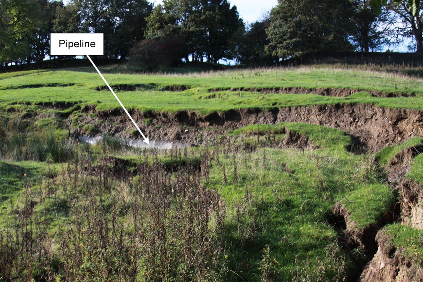
47.2.2 Seismic Hazards
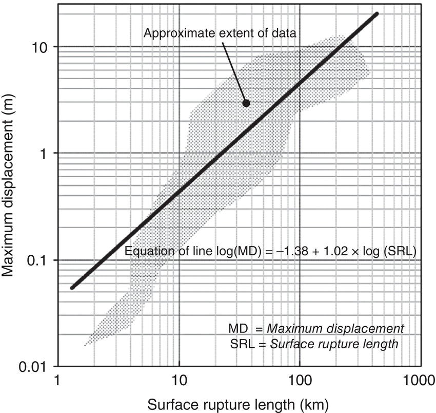
47.2.3 Subsidence
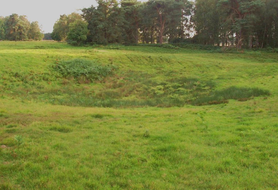
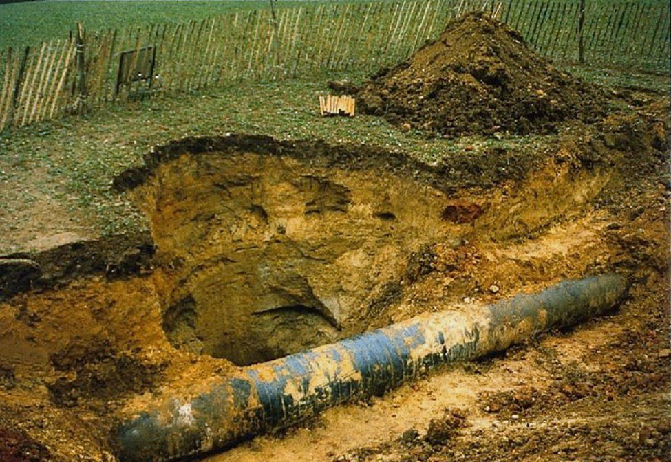
47.2.4 Rivers

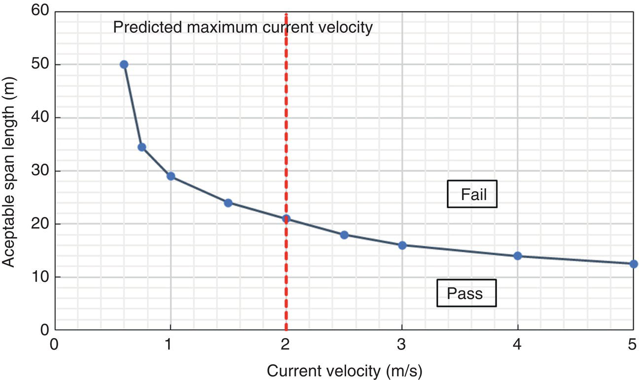
Depth of Cover (m)
<0.5 m
From 0.5 to 1.2 m
From 1.2 to 4 m
Major tidal crossing
1
1
1
Major navigable river
2
3
5
Minor river crossing
5
5
5
47.2.5 Erosion
47.2.6 Additional Types of Geohazards
47.2.7 Morphoclimatic Zones
47.2.8 Other Sources of Loading
47.2.8.1 Civil Engineering Loads
47.2.8.2 Mining Subsidence

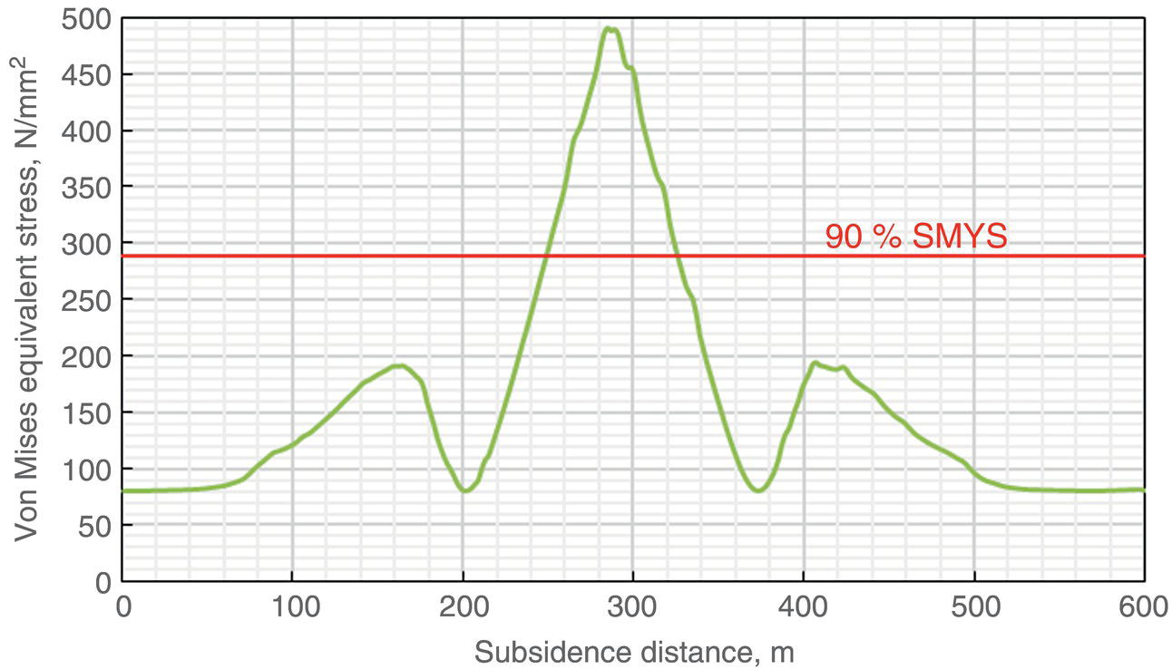
47.2.8.3 Fluid Abstraction
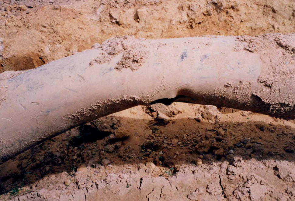
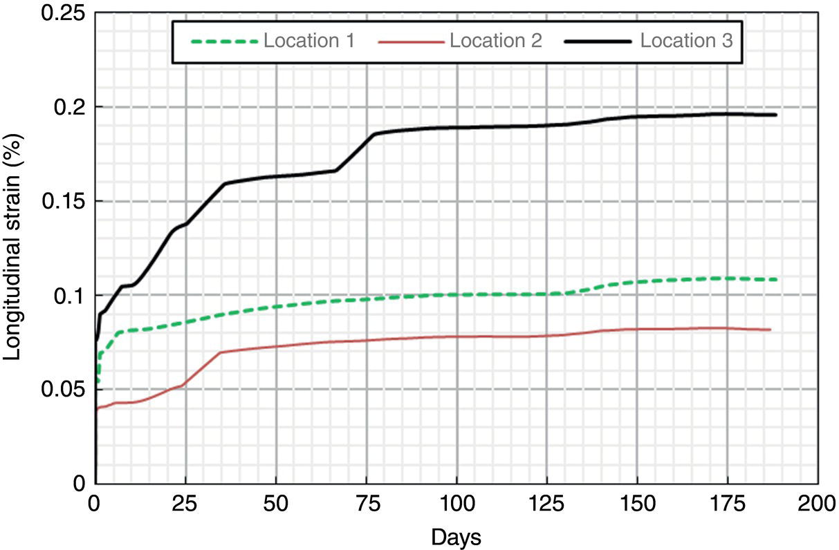
47.2.8.4 Construction Loads
47.3 Regulations on Geohazard Management
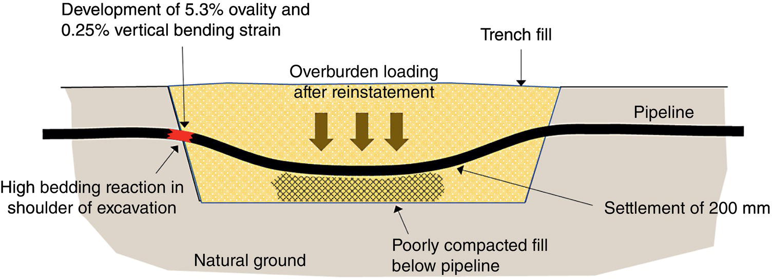
47.4 Geohazards Management Plan
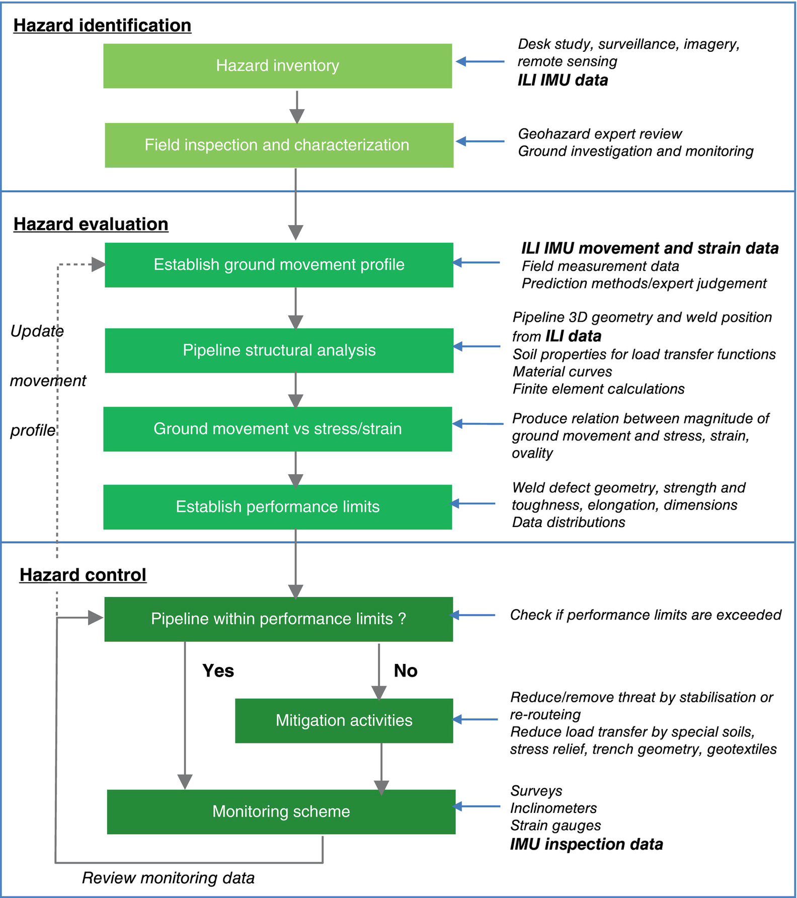
47.5 Hazard Identification
47.5.1 Inspection Methods
47.5.2 Remote Sensing Including LiDAR
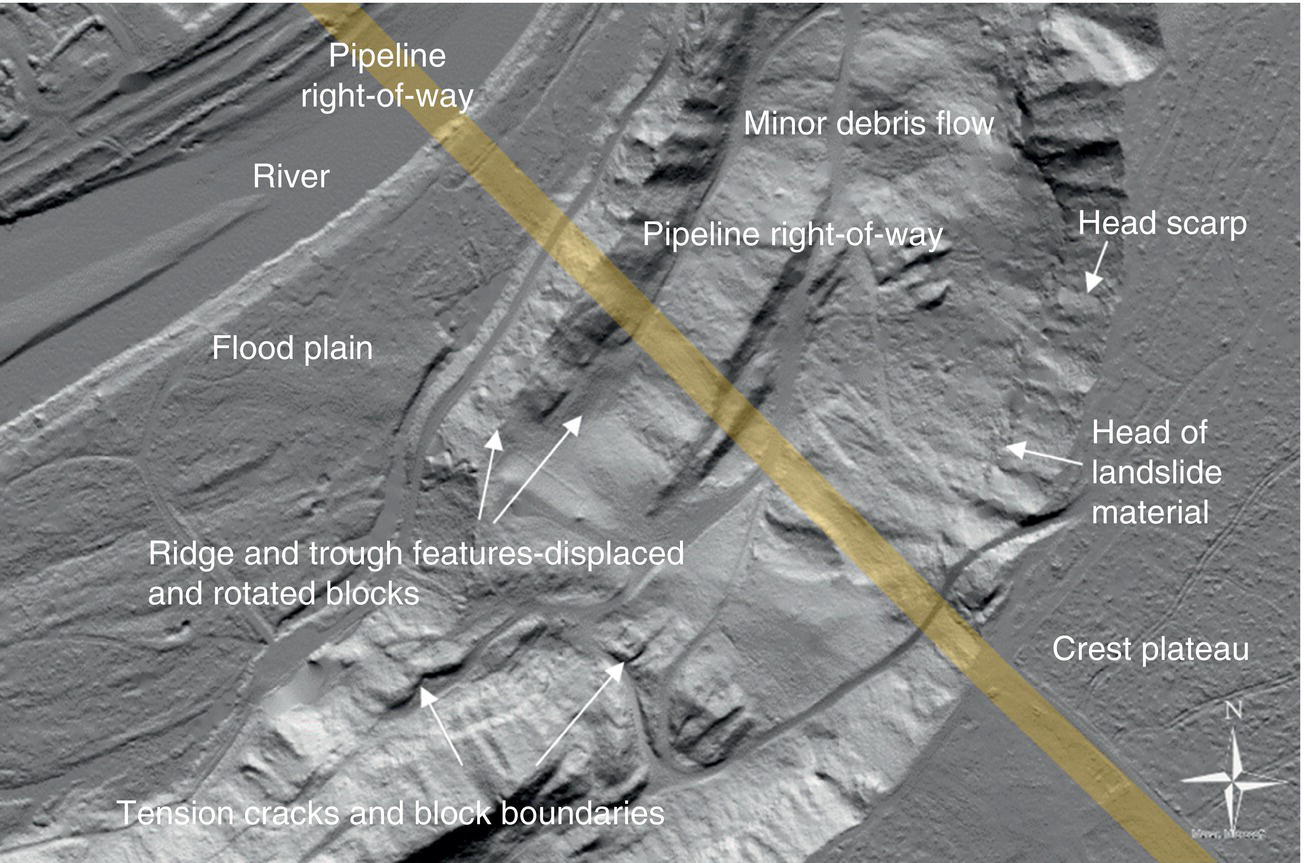
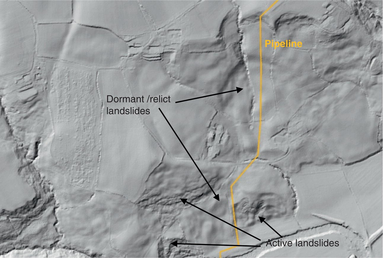
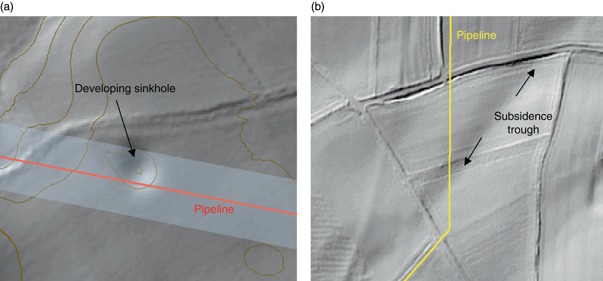
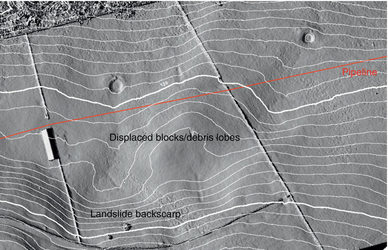
47.5.3 IMU Inspection
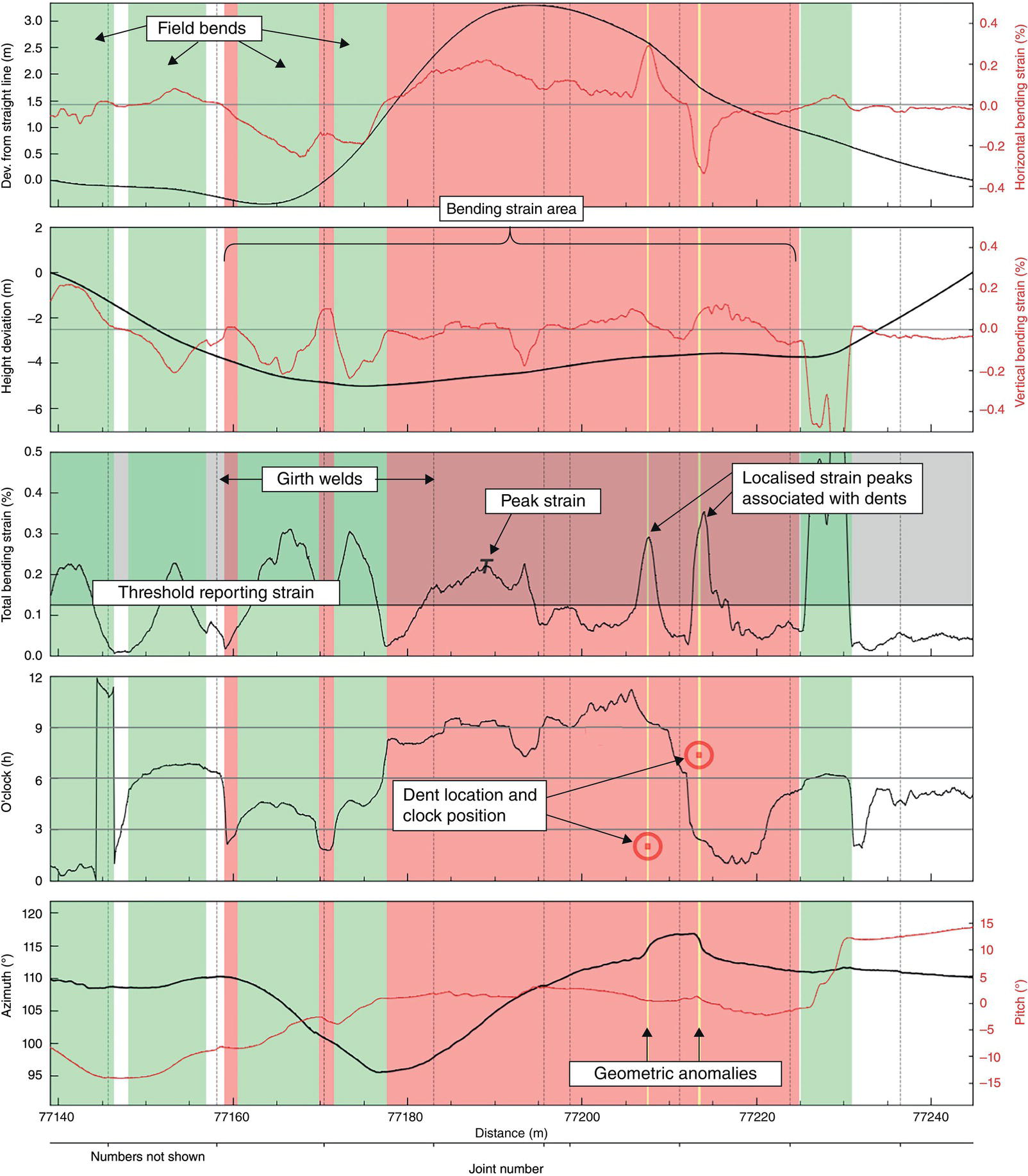
47.5.4 Assessment of Areas of Bending Strain—Screening
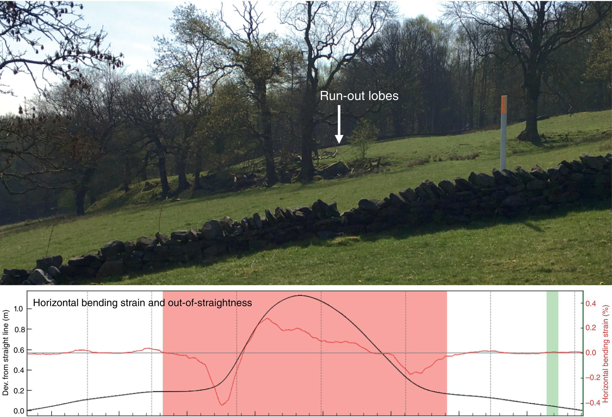
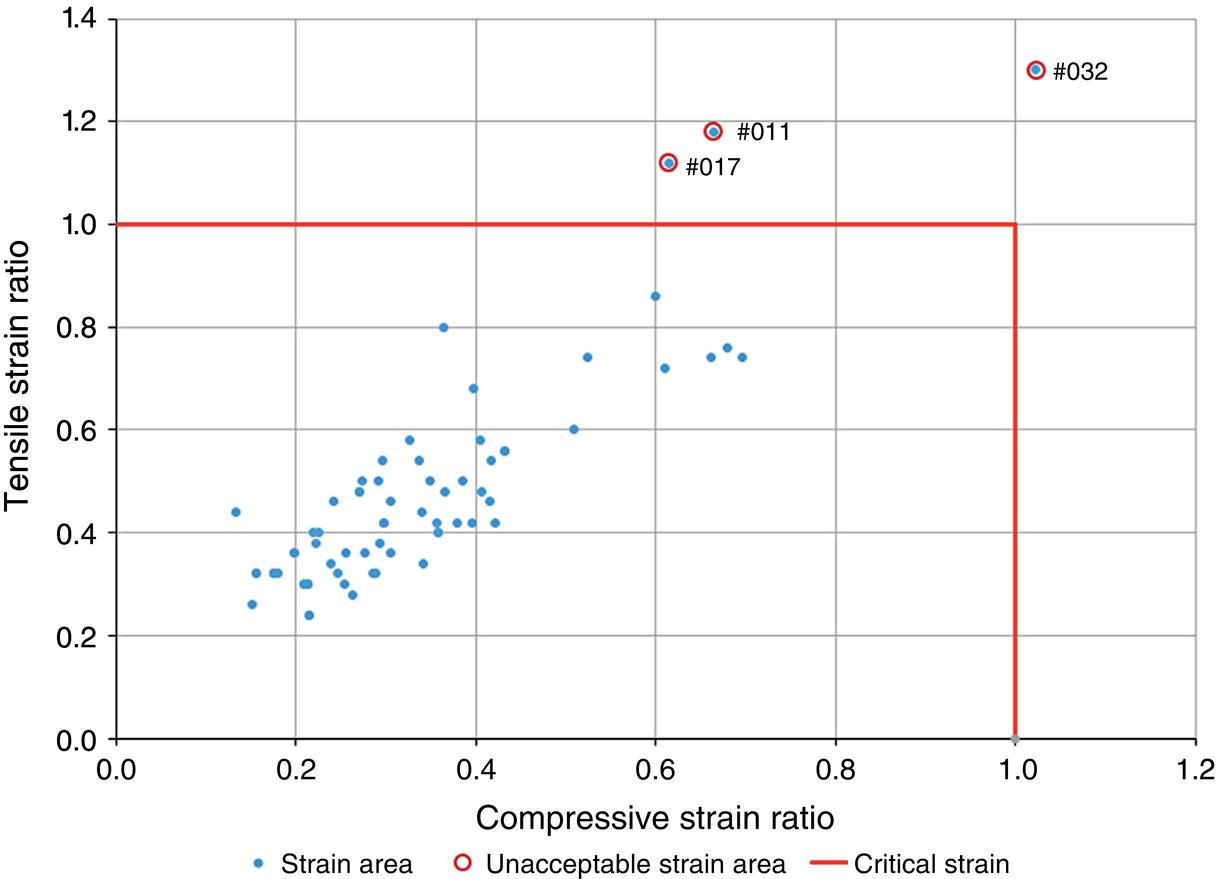
47.5.5 Assessment of Areas of Bending Strain—Examples

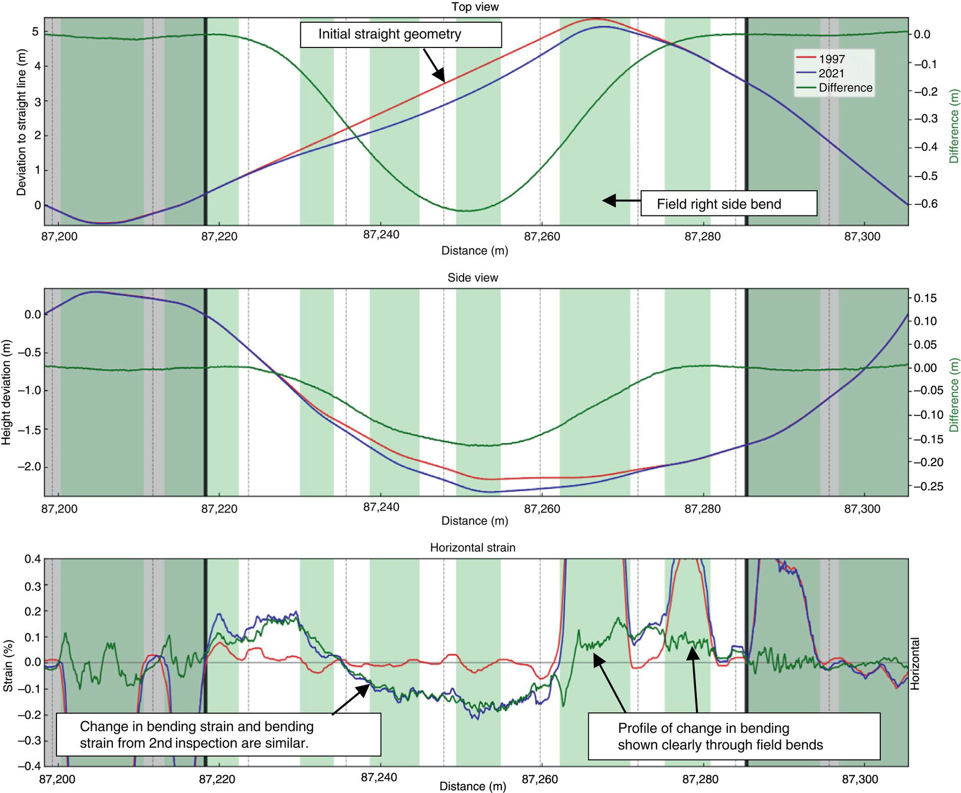
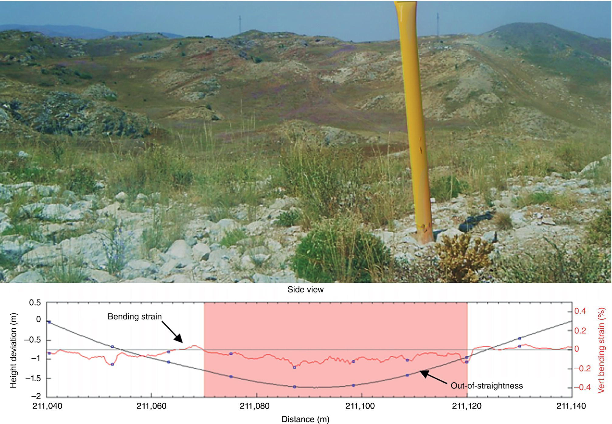
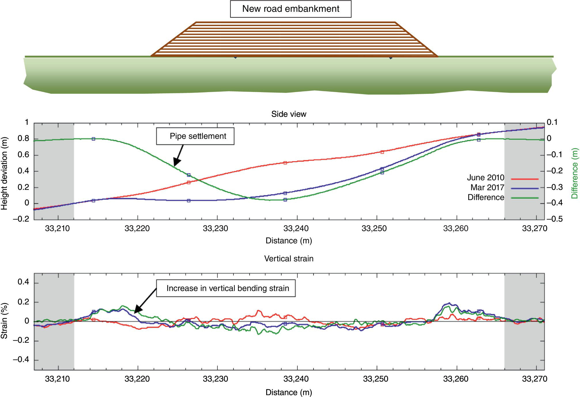
47.5.6 Assessment of Areas of Bending Strain—Construction
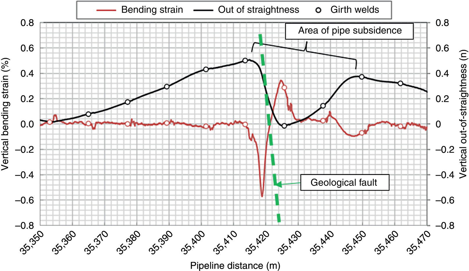

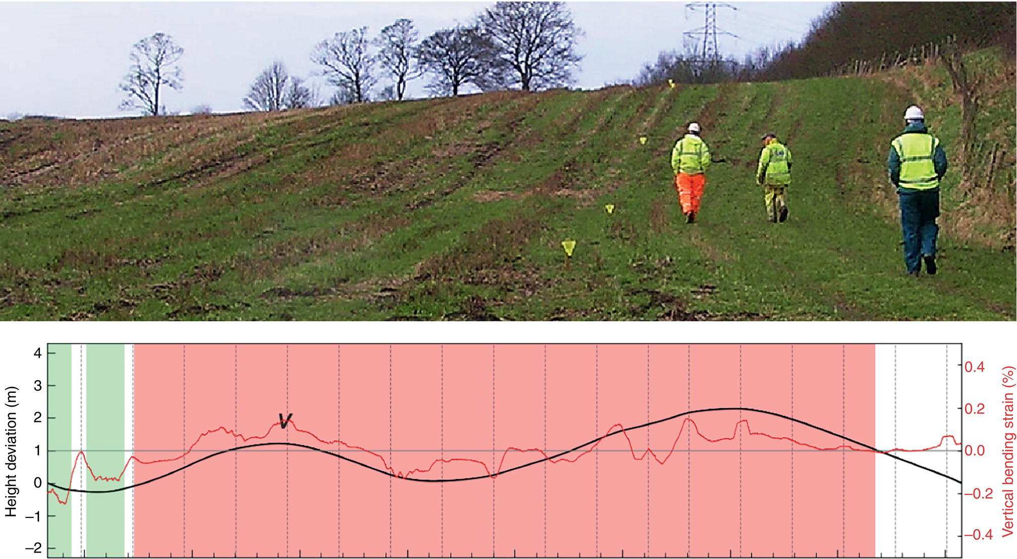
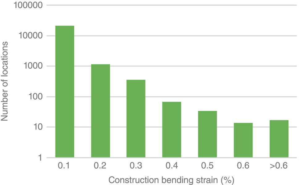
47.5.7 Prioritization of Sites
47.5.8 Use of Bending Strain in Crack Management
47.6 Hazard Evaluation
47.6.1 Ground Model
47.6.2 Performance Limits
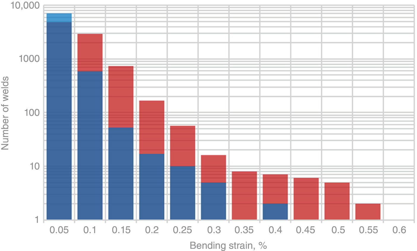
47.6.3 Strain Gauges and IMU
47.6.4 Structural Calculations
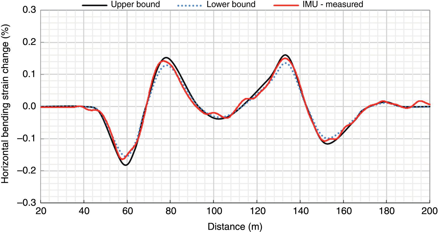
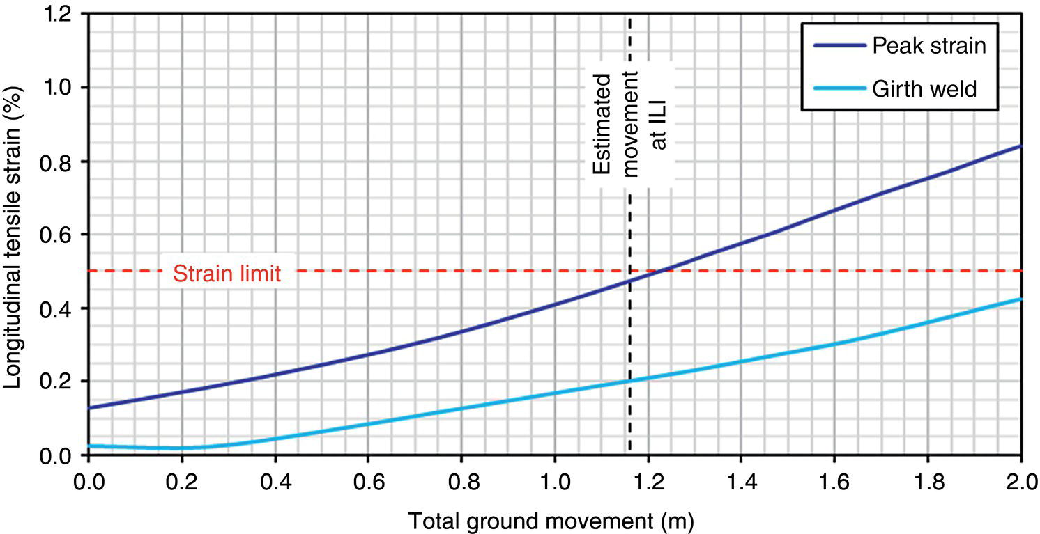
47.6.5 Axial Loading
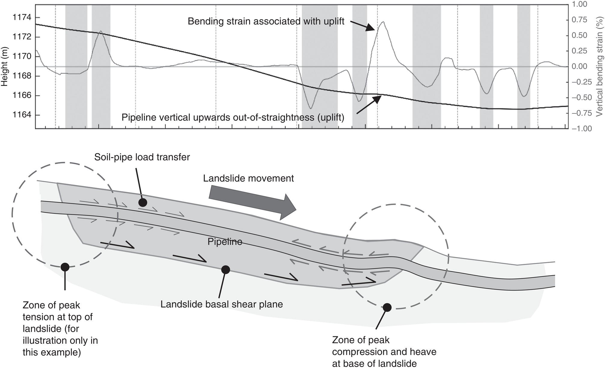
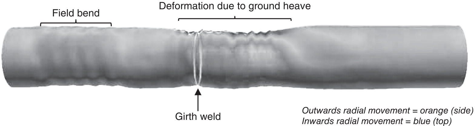
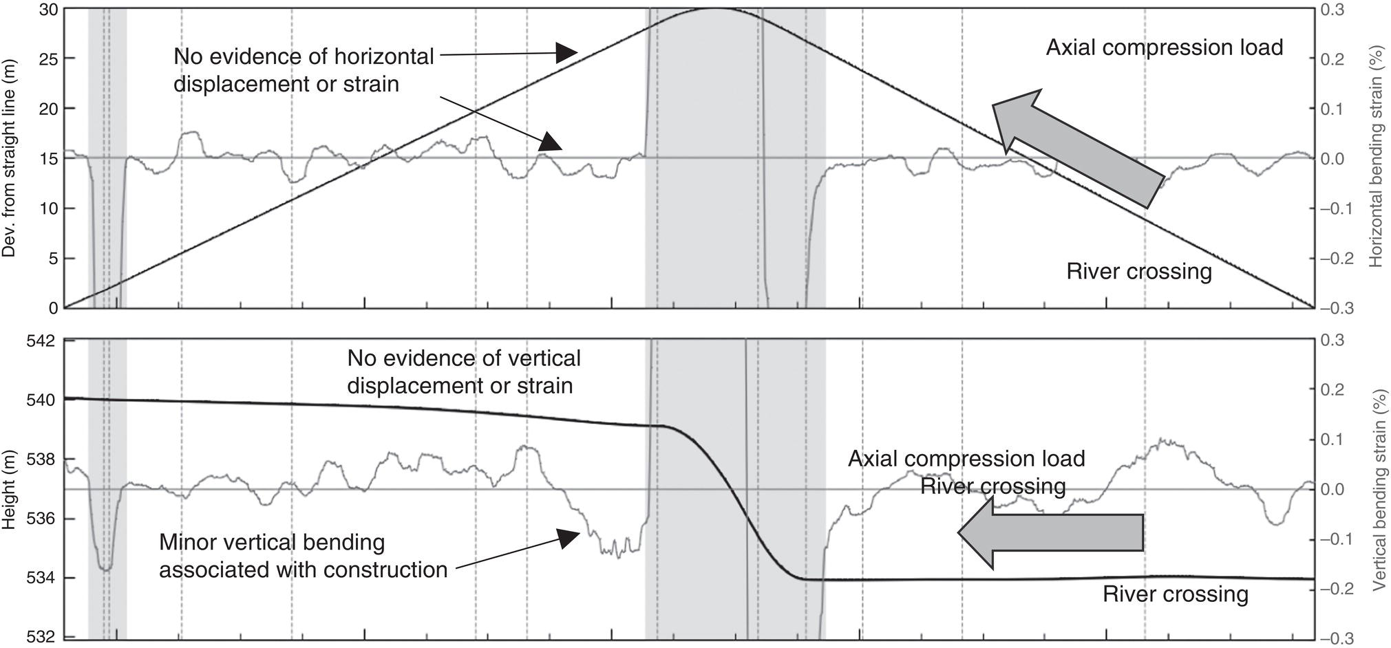
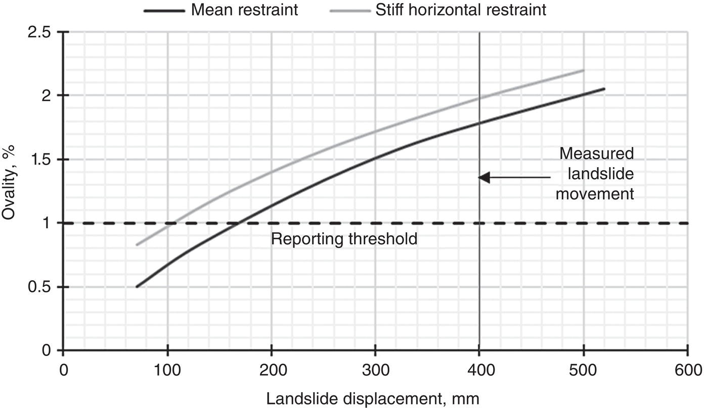
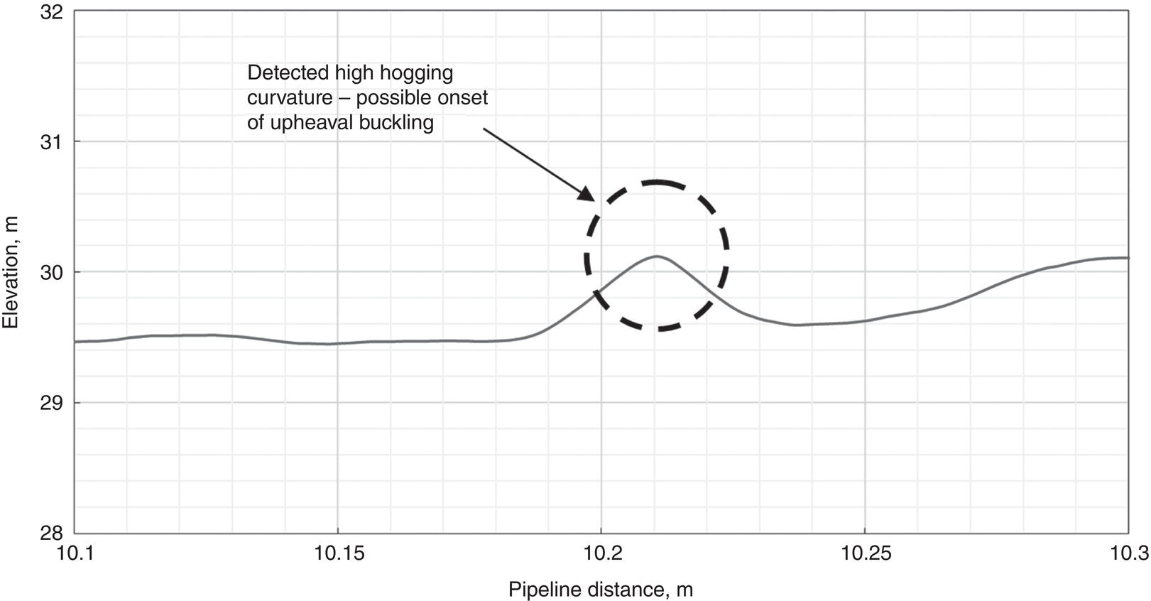
47.6.6 Estimation of Risk
47.7 Hazard Mitigation
47.7.1 General
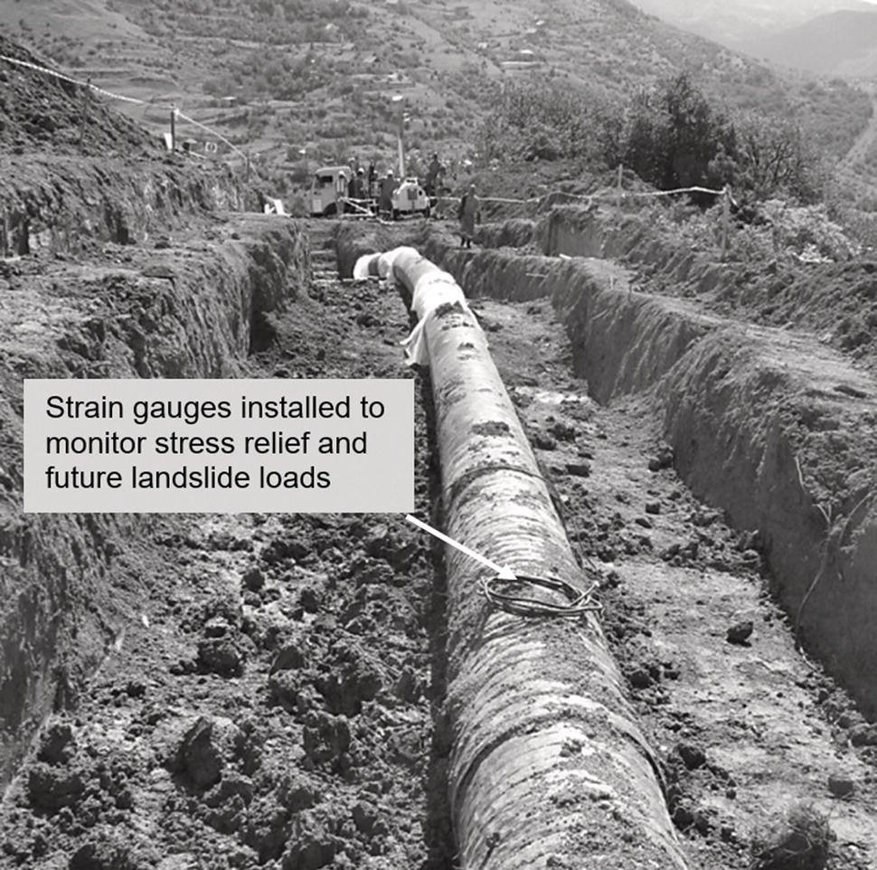
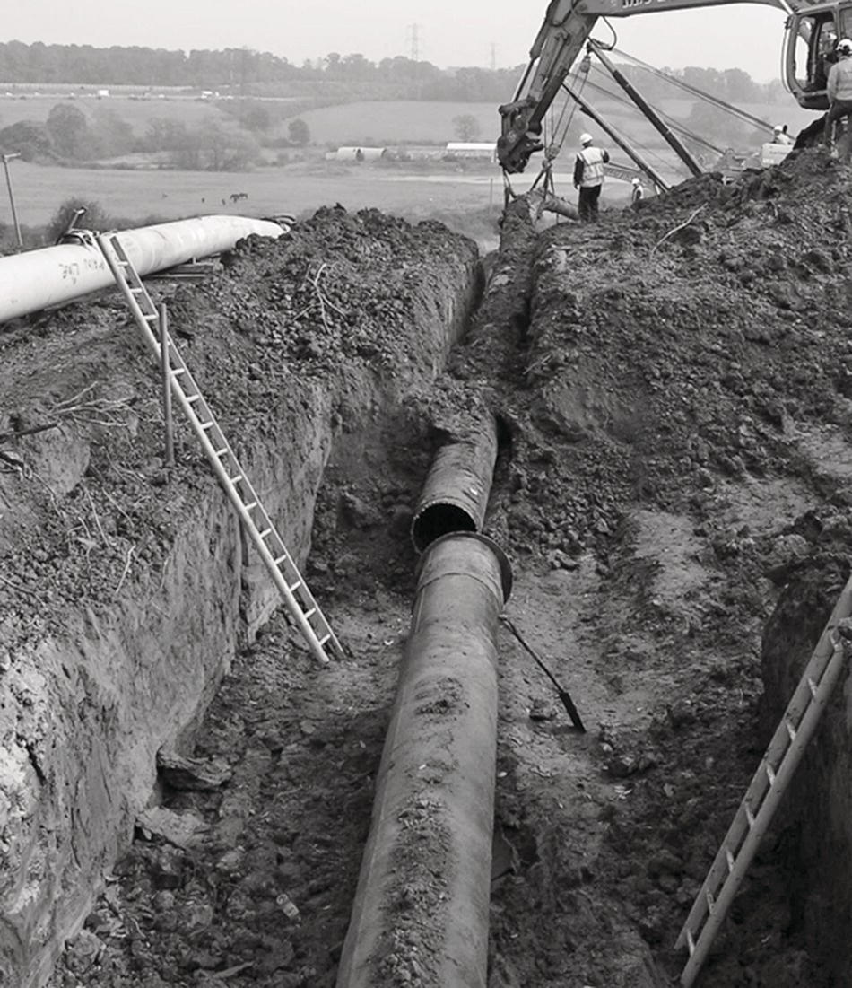
47.7.2 Ground Movement Monitoring
47.7.3 Pipe Monitoring
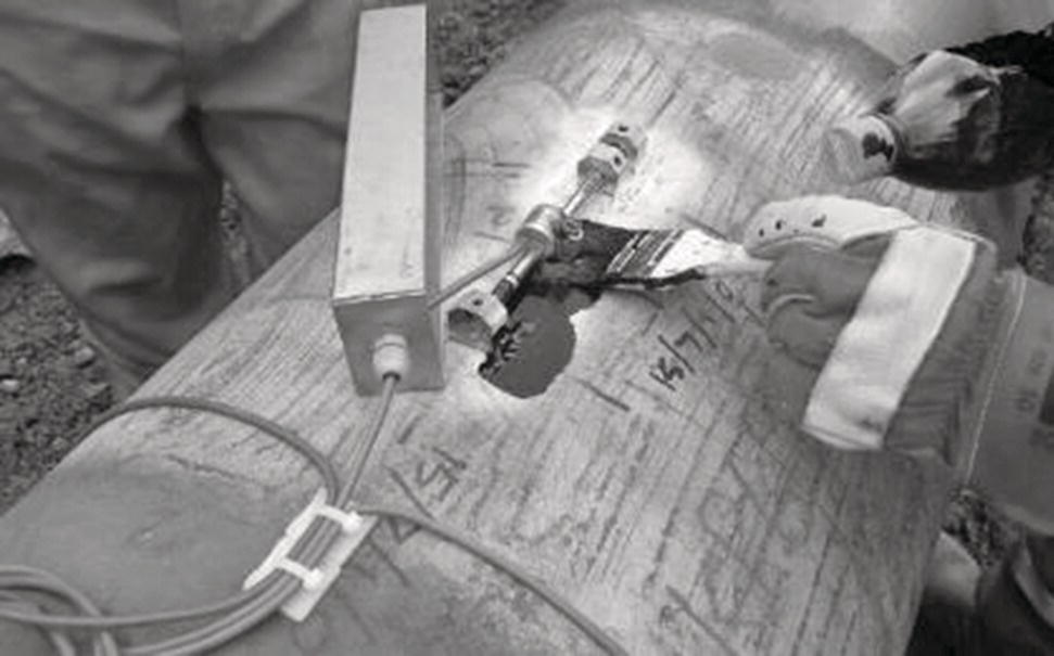
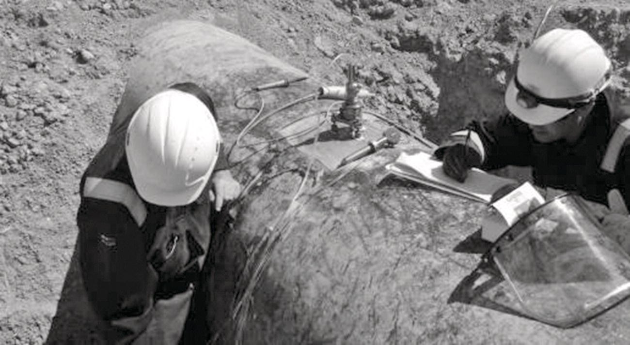
References
Note