Brian N. Leis B N Leis Consultant, Inc., Worthington, OH, USA This chapter considers the circumstances and processes involved in managing an aging pipeline infrastructure. Background to this topic is presented in terms of the high-level factors that drive the pipeline industry, the products it transports, and some of the challenges it faces as supply basins become increasingly remote to the markets. Thereafter, the circumstances and evolution of technology that determine the construction processes and define the initial condition of the infrastructure are reviewed. These aspects are then discussed and evaluated with regard to the threats to pipeline integrity. The development and role of codes and standards is outlined, as is the role of the regulatory framework with regard to actions that affect system integrity. Finally, the processes involved in managing an aging pipeline infrastructure are reviewed as the basis to identify process limitations and related technology gaps. The chapter closes with the finding that the current process that prioritizes defect size could make a step improvement through use of local properties, but this is constrained by a technology gap. A near-term stopgap is suggested, as elaborated in the chapter. The earliest pipelines transporting oil and natural gas in the United States first moved natural gas from a local source to and between nearby houses through hollow logs in Fredonia, NY circa 1825, while oil was transported first near Oil City, PA through a short 2-in. diameter cast-iron system in the early 1860s [1]. Pipelines came into use in Canada in 1862, moving oil from the Petrolia field near the city of Sarnia, ON into the city, with natural gas being transported first by pipeline a year later moving the gas through a cast-iron system into Trois Rivières, Québec [2]. Pipelines have since been increasingly involved in raw energy transportation. However, when lower volumes were required, petroleum products such as oil were also moved from the wellhead to nearby railheads via horse-drawn carts. In those modes of transportation, the product was contained in large wooden barrels, whose significance remains apparent today as the unit of measure for the quantity of liquid being transported or marketed. However, the use of these transport modes diminished as the volume transported grew with demand and the distance to markets increased. Demand grew as petroleum-based products were found increasingly merchantable for lighting and other purposes, and as the population expanded, which over time became focused in larger urban centers. As the demand grew, the locally available supply from nearby shallow wells dwindled, which forced deeper wells and eventually led to the discovery and development of major supply basins. With growth in demand, and the easily accessible product exhausted, the supply basins have become increasingly remote to the markets. More critically, in many such cases, the desired resources (i.e., oil and natural gas) often lie in reservoirs associated with other aggressive fluids and gases, with higher temperatures involved for the deeper wells, whereas very low temperatures and ice or permafrost complicate arctic exploration and production (E&P). While many factors can be involved, where large volumes of oil or gas had to be transported over long distances, pipelines became recognized as the most economical mode of transportation from the wellhead to the market. Such considerations paved the way for pipelines to replace the early modes of shipping, although the barrel remains the metric for the quantity of liquid delivered. Pipelines remain the best method to transport such products when feasible. However, where the geography or other factors make this mode impractical, transport by ship was adopted. As onshore resources near to market became inadequate, E&P moved offshore and into sometimes very remote pristine areas, such as Alaska or further out into the Gulf of Mexico—with safety in those settings being more in jeopardy. This is evident from Figure 41.1 [3], which presents the risk involved in oil and gas E&P and that of other industries in terms of incident likelihood in the y-axis and their dollar consequences in the x-axis, wherein offshore E&P lies along the upper bound of these metrics. Figure 41.1 Risk in energy development versus other scenarios. (Adapted from Stiff [4].) Onshore in the lower 48 US states, pipelines are used to move the imported as well as domestic supplies to market. This is also true onshore in other countries around the world. As the supply basins became increasingly remote, a system of high-capacity pipelines was developed to transport crude and refined products, and natural gas, from the supply points to the market centers, hubs, or terminals. Thus, a cross-country infrastructure of pipelines developed that traverses throughout the United States and adjacent countries, with eventual cross-border interconnects. Such development continues today in the United States, particularly concerning shale E&P and related processing, and also worldwide, wherever demand must be tied into supply. At present, the natural gas transmission system comprises more than 210 natural gas pipeline systems and in excess of 300,000 mi. of interstate and intrastate pipelines [4]. The system that is committed to moving crude and other hazardous liquids also involves a large number of operators but is somewhat shorter, being in excess of 170,000 mi. [5]. As contrasted elsewhere in detail [6], differences exist in the design and components of gas versus liquids transmission systems because of key differences in the products being transported, and the circumstances involved in maintaining efficient operation. Critical in this context is compressibility and the major differences in the phase boundaries of the transported products in pressure–temperature–volume space. Equally important are the terms and conditions of the tariffs and product quality specifications, and the need to keep liquid water out of the systems to manage internal corrosion (IC). Transmission pipeline systems exist “midstream” in the oil and gas value chain that begins “upstream” with E&P and ends “downstream” with a distribution network to the end user. As such, a transmission system comprises end-point and distributed storage in various forms, as well as prime movers, pressure controls, and other related support facilities that include a supervisory control and data acquisition (SCADA) system, and measurement and regulator stations. These system elements can be discriminated with regard to their location and function. These elements are (1) either located at discrete sites (e.g., facilities, compressor/pump stations, storage) or (2) part of the often-remote lineal aspects (e.g., pipeline, mainline valves). Regarding function, and its implications for integrity, the elements either do not involve moving parts (i.e., they are static, such as the linepipe) or they involve moving parts (like prime movers and other equipment). This chapter specifically addresses the network of transmission linepipe and how that linepipe was built into a pipeline. Figure 41.2 Evolution of the steel-making processes. (Adapted from [8].) Logically, supply basins were sought as close to the markets as possible. Pipelines constructed between these points tended to develop first along routes that were most easily traversed, which also targeted the largest markets—tracking the so-called path of least resistance. Early pipelines often traversed open country, such as farm fields. Construction made use of ditching machines and hand shovels, with mechanized equipment used as it became available. The pipeline was constructed beside the ditch as a string and then lowered onto the ditch bottom. A-frames were used to lower-in the pipe string, which gave way to side-booms beginning in the 1930s. Where the ditch bottom was smooth, it also served as the foundation for the pipeline, with native soil returned to the ditch as bedding and padding if needed, as well as cover for the pipeline. Given that the history of pipelines in the United States traces back more than a century, it is instructive to contrast the changes over time, as these affect all aspects of pipelines, from routing and design to construction and operations and maintenance (O&M). Figures 41.2–41.4, adapted from Ref. [7], provide perspective for such changes and indicate the timeline over which these practices were prevalent, specifically with regard to the United States. These figures, respectively, indicate the evolution in the type of steel used to make the body of the linepipe, how that steel was manufactured into linepipe, and how that linepipe has been joined, or otherwise built into pipeline systems. To facilitate later discussion of the evolution over time, each figure has been divided into three timeframes—up through ~1940, which is labeled therein “early,” between 1940 and 1970, which is labeled “vintage,” and beyond 1970, which is labeled “modern.” The last in this sequence of dates, 1970, has been chosen in part because that is when the current regulatory framework was introduced in the United States, and in part because that date can be associated with a transition in steel and pipe making. The first of these dates is somewhat more arbitrary, being chosen to reflect a transition in many aspects of construction, the beginning of a period of change with regard to steel and pipe making, and the onset of a period that opened to the construction of a significant portion of the current pipeline network. Following discussion with regard to Figures 41.2–41.4, this chapter focuses on the pipeline network prior to what has been termed the “modern” era. Figure 41.3 Evolution of in-linepipe production. (Adapted from [8].) Figure 41.4 Evolution of construction practices. (Adapted from [8].) Figure 41.2, adapted from Ref. [7], illustrates aspects of the evolution of the steel-making processes used to make linepipe, over a timeline from circa 1900 through modern technology. The steel-making process is central to pipeline design and its in-service integrity, as it affects the chemistry of the steel, which coupled with processing affects the microstructure and the presence and location of impurities or undesirable constituents (cleanliness). All such aspects couple to control the steel’s flow and fracture response, details for which can be found in Ref. [8]. Significantly, the processing of the steel with regard to rolling and other thermal mechanical (TM) controlled processing can have a beneficial effect on the flow and fracture response, but also can have a negative effect—depending on the TM conditions and history. What follows is a thumbnail sketch of such aspects, which as mentioned earlier have been addressed elsewhere with regard to pipeline applications in great detail [8]. Steel manufacturing in the United States began with the introduction of the Bessemer process in the mid-1800s, which found use for the production of butt-welded, lap welded, and seamless (SMLS) pipe. The open hearth process quickly followed (1870s–1880s) and evolved into the primary method for steel production in the world by the early 1900s. These developments were followed by the electric furnace (1899), which began production between 1900 and 1910. Subsequently, basic oxygen steel making was implemented by the mid-1950s, and by 1969 accounted for nearly half of the annual steel production. Of these processes, steel produced for linepipe through the 1960s included the open hearth, basic oxygen, and Bessemer processes, with electric furnace steel used only in limited quantities. Prior to the 1960s, ingot casting and hot rolling were typically used to produce plate and skelp for linepipe production. Both partially deoxidized (semi-killed) and fully deoxidized (killed) steels were used, and depending on the deoxidation practice, ingot structural soundness varied. During this same period, higher yield strength materials were introduced, wherein the primary method used to increase strength was increased alloy content, which tended to increase the hardness and reduce the weldability. Pre-1960 steels have higher residual impurity levels and more frequent internal anomalies as compared to post-1970s production. In many cases, the impurities are strung-out parallel to the pipe surfaces, which while they have limited influence on strength, they can act as initiation sites for some forms of corrosion and/or cracking. From the late 1960s and into the 1970s, several major improvements were implemented in steel manufacturing and in plate/skelp rolling. Microalloyed steels with additions of niobium, vanadium, and other elements, coupled with improved steel rolling practices (controlled rolling) and improved impurity controls (desulfurization, inclusion shape control, vacuum degassing), resulted in “cleaner” steels with higher yield strengths, increased toughness levels, and improved weldability. Continuous casting (concast) began to be used in the same time period, further improving steel quality, while providing more efficient production. Nevertheless, centerline segregation in the concast strand can remain a concern in demanding applications (e.g., [8]). Further developments in steel production and rolling practices came in the 1970s and 1980s through control of steel microstructures, additional rolling method improvements (accelerated cooling), and chemical additions. These gave rise to higher yield strengths, quantified by the “grade” of steel, which means stronger pipe for the same wall thickness. For linepipe, grade is denoted by the prefix X followed by the specified minimum yield stress (SMYS) in ksi units. These changes in the steel also led to fewer impurities, and improved weldability. Sophisticated steel manufacturing controls and improved nondestructive inspection (NDI) systems have also resulted in a reduction of material-related anomalies found in modern linepipe, with Grade X100 now considered a commercial product. Key in this context is that steel has evolved to address the needs of the pipeline industry with significant quality and related developments being triggered by the need to manage concerns such as brittle fracture and running ductile fracture. Development was also spurred by the desire to manage capital expenditures (CAPEX), which is evident in the increase in grade as mentioned earlier, which allows reduced wall thickness and so increased productivity on the spread during construction. It is also evident in changes in the rolling mills to provide wider plate and skelp, which permit producing larger diameter pipelines, which diminishes the time on the spread, as well as the scope of related O&M work, to help manage operating expenditures (OPEX). Figure 41.3 illustrates the evolution of in-linepipe production. This involves transforming flat stock as plate or skelp into either a cylindrical shape that is closed by a longitudinal seam, which can be straight or helical, or a SMLS cylinder. Depending on how the linepipe is produced, and the need for dimensional control, pipe can be cold expanded up to 1.5% following completion of the pipe-making process. Thereafter, it is tested and accepted, then beveled and otherwise prepared, in accordance with contract and other specifications and regulations. Early pipe-making processes noted in Figure 41.3 include furnace butt-welded, lap and hammer welded, low-frequency (LF) electric resistance welded (ERW), flash weld, and continuous butt-welded, with the latter still in use. Subsequently used processes included single-submerged-arc welded (SAW), and some early variations on SMLS pipe, with high-frequency ERW (HF-ERW), and double submerged arc welding (DSAW) coming thereafter. The DSAW process has been used to produce both straight seam as well as spiral (helical) seam pipe. Of these, modern construction relies on SMLS pipe and the HF-ERW and DSAW processes. In contrast, the “early” category involves several long-since-abandoned processes, as does the “vintage” category. The vintage category can be viewed as a period of transition away from steel and seam making practices that were prone to process variation and production upsets, which lead to seam-related defects. Thus, as noted with regard to the evolution of steel, changes have come in pipe making to improve quality. Changes also have been made with regard to capacity of the mills to produce larger diameter, and heavier wall pipe, as needed to manage CAPEX and OPEX. Finally, in analogy to Figures 41.2 and 41.3, Figure 41.4 illustrates the evolution of construction practices that have been used to join the linepipe, and to create the directional changes needed to track a routing via bending. It is the evolution in practices to join linepipe, and to create the needed directional changes that account for the improvements in pipeline construction—much of which has been driven by the desire to control CAPEX upfront and the OPEX over the life cycle of the pipeline network. As early practices were found to be problematic with regard to managing CAPEX or OPEX, they were quickly discontinued, with the related issues promptly resolved. In this context, it is not a surprise that much of the vintage construction remains in service today without issue. For this reason, a later section illustrates novel construction practices, wherein their utility and continued serviceability are evident. Early joining practices relied on threaded collars, which were used on the earliest crude oil pipelines, with mechanical couplings coming into use as well. The earliest welds were made via the oxy-acetylene process, which as time passed incorporated a backing ring below the girth weld. The use of flanged connections, which were approved by the ASME circa 1894 and require welding to attach the fitting to the linepipe, followed as the early welding technology was more broadly adopted. Of these, only flanged connections continued in use beyond the period denoted “early” in the figure. Figure 41.4 also indicates the role of wrinklebends, which were used with other historical field-bending practices, such as welded segmented (miter) bends, through the 1940s. As evident in this figure, the period denoted “vintage” also was a time of transition from the early practices to those in use today—such as submerged arc and other more advanced methods that in modern applications are used under automated conditions and work in conjunction with line-up clamps. The transition to and through the vintage era on into the modern era also gave rise to the use of machine-made field bends, with such machines emerging in the 1940s and continuing to develop since, for straight as well as helical seamed pipe. Directional drilling also traces back to a similar timeline, and has recently become viable for long-distance drills involving large-diameter construction, providing a viable ecofriendly approach to deal with routings sensitive to such issues. And, where difficult routings move through rocky and hilly terrain, bedding and padding and other trench-bottom technology have evolved largely in the modern era to manage such construction. The transition through the vintage to the modern era opened the use of cathodic protection (CP), beginning in the 1940s, the use of which expanded until it was eventually mandated in the transition into the modern era. As the threat of corrosion was recognized, over-the-ditch coating methods also went into use in the 1940s. Step improvements in coating technology began with the early versions of today’s resin-based formulations that appeared in the 1970s. Continuous improvement in these technologies, coupled with the realization that appropriate preparation was as critical as the nature of the coating system, and its application, have now effectively controlled external corrosion (EC). Likewise, tools and technologies have evolved to better manage IC, which range from designed inhibitors through internal coatings. Field applied coatings likewise have improved to deal with surfaces left uncoated in the mill to facilitate girth welding. Finally, the transition through the vintage to the modern era gave rise to significant changes in pipeline system monitoring and control. The first monitoring via in-line inspection (ILI) came late in the transition from the vintage to modern era, in 1965, which since has gone through several generations of development, and expanded its initial role with regard to metal loss to deal selectively with cracking, mechanical damage, alignment, and deformation. SCADA introduced initially to better track product delivery was subsequently coupled with sensors, remotely controlled valves, and system-specific software and found other uses, such as tracking pressure and other operational parameters, which facilitate better control, and also leak detection and outflow control. The evolution in the aspects of pipeline systems that were apparent in Figures 41.2–41.4 has been “fueled” by the competitive need to manage both CAPEX and OPEX as pipeline companies expanded their capacity in the competition to meet the ever-growing demand for energy. In this context, that competition to get off the construction spread and into production led to improved steels that could be produced in stronger grades that also were more weldable. Such steels also were tougher and had lower transition temperatures, whose use opened to mechanized more controllable welding processes. The push to build more efficient systems over the life cycle led to improved operational controls as well as better coating processes, and improved control of CP. As such, overall system safety has the potential to improve as a consequence of the evolution evident in Figures 41.2–41.4. The extent of the expansion to meet the market demands is evident in Figure 41.5, wherein the incremental mileage constructed is shown in the left-y-axis as a function of the period of construction over the interval from before 1920 into the new millennium, which is shown in the x-axis. The right-y-axis presents the cumulative mileage constructed over this same interval. Figure 41.5a shows these data for interstate natural gas transmission pipelines, whereas Figure 41.5b shows the corresponding data for interstate hazardous liquid transmission systems. The timeline in these figures denoted >2000 includes results up through 2010, while the timeline used in Figures 41.2–41.4 ends at the start of the new millennia. Little is lost in this context as that decade saw little technology growth—except for developments in inspection capabilities. Differences also exist between Figures 41.2–41.5 with regard to the start of the trending. However, again little is lost because the accumulated mileage prior to the 1920s represents a trivial fraction of the total natural gas and hazardous liquid mileage thereafter. Inspection of Figure 41.5a and b indicates that the “early” era comprises a nominal fraction of both the networks. It is apparent from Figure 41.5a that the natural gas system experienced strong growth beginning in the 1920s, which culminated in the fastest growth in the 1950s and 1960s at a relative rate that has since not been matched. The trends in Figure 41.5b indicate that the hazardous liquid system also experienced steady incremental growth since the 1920s, which led to the fastest growth in the 1950s and 1960s, that like the natural gas system its growth has been leveled and steady since the 1960s. As such, it is not surprising that the amount of mileage split between the periods designated in prior discussion as early, vintage, and modern, is comparable. This is evident by comparing the split mileage built within these three timeframes, which is apparent in the corresponding sets of numbers added into Figure 41.5a and b. For the natural gas system this split is 6% prior to 1940, with 52% from 1940 to 1970, and 42% since 1970, while for the hazardous liquid system construction prior to 1940 involved 7%, with 49% in the interval from 1940 to 1970 and 44% thereafter. The horizontal lines shown in Figure 41.5a and b correspond to one-half of the current total system mileage. The vertical lines that drop from its intersection with the cumulative mileage trend to the timeline shown in the x-axis indicate that for the hazardous liquid and natural gas transmission systems roughly one-half of those networks were constructed prior to ~1961, with about two-thirds of these networks being constructed prior to 1970. Recognizing that the amount of the network built in the “early” era is but a nominal fraction of the total network, it is evident that roughly one-half of the US transmission network was built in the era designated as “vintage” in the context of Figures 41.1–41.3. Figure 41.5 indicates that the step increase in mileage for the natural gas system began in the 1950s, which is paralleled by the growth in the liquids mileage. While length provides an indication of transmission pipeline system expansion, the volume transported provides a better measure of its growth. Volume or capacity is controlled in part by linepipe diameter, which is dictated by mill capacity to produce wider skelp and plate. It is also controlled in part by pressure, which under working stress design (WSD) (e.g., [10]) is controlled by SMYS, or equally the pipe grade. Suffice it here to note that by the start of the 1960s, the mills were broadly capable of producing pipe in Grade X52 for which SMYS is roughly double that for Grade A, with diameters in the order of 30 in. (or more)—much larger than several decades earlier. In this regard, the capacity per unit length increases with the square of diameter and linearly with pressure. Thus, even though the incremental length per decade remains flat for these transportation systems since the 1970s, the network capacity has increased. Considering that diameters up to the order of 48 in. have entered service in the United States in grades up to X80 since then, an almost fourfold capacity increase has occurred relative to a 30-in. X52 pipeline, which is otherwise transparent when capacity is assessed in terms of mileage. Figure 41.5 Analysis of construction mileage relative to year built. (a) natural gas transmission lines, (b) hazardous liquid transmission lines. (Derived from raw data in Ref. [10].) Pipe diameter affects the wetted area on the inside diameter (ID) surface and so increases the threat of ID corrosion. It also affects the outside diameter (OD) surface area that must be coated and protected to control the threat of OD corrosion. Accounting for this difference in surface area over time should be considered as improvements in the Pipeline and Hazardous Materials Safety Administration (PHMSA) database lead to a more comprehensive framework and better quality results free of nulls. Until then, mileage remains the only viable metric to assess expansion and normalize trends over time. It follows from Figure 41.5 that roughly one-half of the total transportation network has capitalized on the evolution in steel and linepipe production, and the technology and schemes used to build them in what has been called the modern system. What does this imply for the remainder of the transmission systems constructed prior to 1970? There are two basic approaches to address this question. The first is by analogy to the circumstances evident for parallel applications, such as other transportation infrastructure, systems, and components. The second is by direct analysis of the oil and gas transportation infrastructure and systems. Both approaches will be considered in turn. Consider next parallel transport systems whose infrastructure involves components whose age spans many decades, as occurs for some commercial aircraft and ground vehicles and some pipelines, and portions of other transportation systems, such as bridges and rail transport, whose age approaches that of early pipelines. Some parts of the transportation infrastructure, such as bridges, share the same design basis that is used for pipelines. Bridges, pipelines, and many other structures, initially relied on WSD, wherein a factor of safety was applied to the allowable stress to achieve a safe margin against uncertainty. As time passed, WSD gave way to plastic design or ultimate strength design (USD) for many new bridges and other structures (e.g., [11]). The virtue of USD was that it capitalized on the significant reserve strength evident in the postyield response of typical early-vintage construction steels. It was accepted into practice, even though it offered less reserve capacity as compared to WSD, and is accepted also as a design basis for pipelines in a few countries. Reliability (risk)-based design (RBD, e.g., [12]), which relies on a probabilistic view of structural loading and resistance, also has found favor for structural design in some countries. Canada and a few other countries also allow RBD for pipelines. However, in the United States, pipeline design remains tied to the WSD concept, as does general boiler and pressure vessel design. Other transportation systems (such as the rail and air transport systems) operating in most countries worldwide, also parallel key aspects of pipeline systems in many ways. Like pipelines, such systems provide for long-distance transport of commodities, but unlike pipelines also provide for public transportation. Similar to a pipeline, the paired ribbons of rail that are the backbone of railroad systems are not structurally redundant—if one of the pair of rails fails it is quite possible that the train will derail. And as for a pipeline, such failures can be as catastrophic depending on where the failure occurs and what commodity was being transported. In contrast to rail and pipeline systems, designs underlying air transport seek structural and subsystem redundancy. Yet even though redundant in concept, related failures occur in air transport causing casualties. Human factors likewise contribute to such failures, as they have in some pipeline incidents. As for pipeline systems, both the rail and air transport systems rely on periodic inspection to detect system faults prior to their becoming significant. Both rail and air transport systems are “damage tolerant” (e.g., [13]) in that they continue to operate even though cracks have formed and are growing in structurally critical elements. Both rail and air transport systems are subject to periodic reinspection and condition assessment. Finally, both rail and air transport systems continue to operate equipment and facilities provided, they are maintained and so “fit-for-service” (e.g., [14]) and also “fit for their intended purpose” (e.g., [15]) in that system. However, both rail and air transport systems also consider functionality and efficiency and in some cases will “retire assets for cause” (e.g., [16])—where that action can be motivated by brand concerns, inefficiency, and other considerations, including structural reasons. Competitive drivers also can lead to the sale of assets and to modernization in the rail and air transport industries, just as they have for pipeline systems—or for any other business. It follows that pipelines built under conditions prevalent in the eras defined as “early” or “vintage” can be as viable as those built in the “modern” era as long as they are fit-for-service and for purpose. This is clear in the observation that some cars and big-rig trucks continue to operate for many hundreds of thousands of miles, whereas absent adequate maintenance they could fall short of their expected design life. Because a vehicle is old does not mean it is unsafe, but it can mean that it could require more care, or might not be as fast as its modern counterpart. This also applies in the context of vintage aircraft, many of which are still in service, but for brand reasons, economics, and other considerations they do not operate in the fleet of a major US carrier. This same brand-motivated decision is made when a two-year-old car is sold solely because the owner does not want to be seen in an “older” vehicle. While early or vintage pipelines are analogous in most ways to other early transportation infrastructure that remains in daily use today, whose serviceability depends on adequate maintenance, the best metric of serviceability over time is a quantitative analysis of incident statistics. For pipelines, the most comprehensive basis for statistical analysis and incident trending is the pipeline incident database that has been developing since 1971 under the management of the PHMSA. The PHMSA functions under the US Department of Transportation (DoT) [17], which is responsible for all modes of transportation, such as motor carriers (under PHMSA) and air transport (under the Federal Aviation Administration). PHMSA’s pipeline incident database is publicly available and can be downloaded directly from the PHMSA website [9]. Fundamental to any statistical analysis is the quality and consistency of the data, and which data should be pooled or parsed for the purposes of a given analysis. A check of the PHMSA website indicates that their database has been packaged over time intervals during which the definition of a reportable incident (e.g., see [9]) and their input form and scope (e.g., see [18]) remained constant. As pipelines became increasingly encroached and other factors such as the growth of social media came into play, the sensitivity to the consequences of an incident has increased. Such factors have prompted changes over time in (1) the threat categories used, (2) the criteria used to define a reportable incident, and (3) the scope of data that must be reported. It must be noted in this context that as reporting criteria become more stringent, an event that might not have been reportable in past becomes reportable. More stringent criteria open to a bias toward increased incident frequency as time passes. Because the scope of the data required to offset this bias was not always a required input, and so is often not available, either this bias remains or the database must be culled to exclude it—which precludes trending over time. Over the period since 1971, three major changes can be identified in reporting structure and requirements, which can complicate trending, and attempts to offset any bias due to increasingly stringent requirements. Data quality issues also exist, as do many nulls (or empty reporting cells), which also can affect the utility of the trending. As nothing can be done to resolve the data quality concerns, the results are used as is without regard to the possible effects of the nulls. Because the focus is a possible effect of the era of pipeline construction on the incident rate for the onshore pipeline system, the construction or manufacturing data listed in the PHMSA’s database for onshore interstate pipelines has been pooled and then sorted by construction era as “early” (<1940), “vintage” (1940–1970), and “modern” (>1970), specifically for the liquid pipeline system. The raw outcomes were then normalized relative to the amount of mileage constructed in each of those eras, as reported in Figure 41.5b. Such analysis has been done with regard to the incident data for the modern era up through 2010, as well as up through 2002, because at this time there was a marked shift in the reporting requirements for the liquid system. This analysis was done with regard to the elements of a pipeline system that differ with regard to location and function. That breakdown with regard to location parsed discrete elements (facilities such as stations, tanks, etc.) and the lineal element (including the pipeline and its mainline valves (MLVs)). The discrete elements were further sorted by function with regard to static, such as tanks, versus dynamic, which covered equipment and related components. Because there were no clear trends across these parsed elements, only the results for aggregate system are presented in Figure 41.6. The y-axis in this figure is the mileage-normalized incident frequency for each of the construction eras, which are parsed on the x-axis. Each era in this bar graph includes two results—the first represents the data evaluated through 2010, while the second represents the data evaluated through 2002, when much more stringent reporting criteria for leaks in hazardous liquid lines were introduced. The results of the quantitative analysis of the hydrocarbon transportation infrastructure shown in Figure 41.6 do not indicate that the portions of the pipeline system constructed in the “vintage” or the “early” era are more prone to incidents. It is evident in Figure 41.6 that the difference in the relative fractions of pipelines constructed in the vintage and early eras is small, with the incident fraction for the vintage system being ~5% less than for the early construction. While there is a modest decrease in the relative fraction of reportable incidents moving forward in construction era from early to vintage, Figure 41.6 indicates that the relative fraction of reportable incidents increases sharply moving into the modern era of pipeline construction. Contrasting the results for the database before and after the transition to more stringent reporting requirements circa 2002 accounts for roughly one-third of this increase. This outcome opens to the question: what accounts for the remaining upswing in relative incident frequency for modern construction? The results in Figure 41.5b do not indicate that this can be traced to a surge in construction, which could open to the need for contractors and so introduce a less experienced workforce. Further trending of the modern construction era indicates that while other changes leading to more stringent reporting occurred within this era, they played a minor role if any in the upswing in relative incident frequency for the modern construction. Rather, the results of trending for the modern era in 10-year increments suggest there was a period of learning and/or adaptation as the US industry incorporated the many improvements in steel making that were phased in circa 1970 (see Figure 41.2). For example, the transition from LF-ERW to HF-ERW longitudinal seam production that began in the early 1960s and was completed in the United States in the early 1970s (see Figure 41.3) experienced some developmental issues into the 1970s. Likewise, as the use of emerging construction practices broadened, there is evidence in trending the data that this aspect also experienced some developmental issues in the 1970s. If the trend evident for the 1970s was more like that of the 1980s or the 1990s, then the upswing evident in relative incident frequency for the modern construction era is diminished—with little difference evident over time. Figure 41.6 Incident frequency parsed by construction era for interstate liquid transmission. It follows that parallel transportation systems share comparable traits with no clear evidence that era of construction or age affects the mileage-normalized incident frequency for the hydrocarbon pipeline system assessed with regard to Figure 41.6. In contrast, a major failure within the pipeline industry and the parallel transportations systems considered earlier often opens to the discussion of a system’s or component’s age. Although the risk to the public or the environment associated with the trends in Figure 41.6 is not quantitatively out of line with other day-to-day risk exposure, it is often involuntary exposure. While such events are infrequent, such exposure can lead to environmental issues and loss of life, whose cost to the pipeline operator is not trivial. Recognizing this, since the 1930s the industry has worked to develop consensus standards and company specifications and protocols for O&M. And, as the public and environment can be adversely affected, a regulatory framework was introduced circa 1970. These aspects and their implications with regard to older pipelines (i.e., pipelines constructed in the vintage and early eras) are considered next. It is evident from Figures 41.2–41.4 that today’s modern pipeline systems have evolved greatly, from routing and design, on through construction, and into O&M. The design codes, related specifications, and regulations have likewise evolved. What began in the 1800s based on rudimentary schemes has evolved and now is directed at system safety over the life cycle of the system. Steel has replaced wood and cast iron, and couplings have been replaced by automatic welding, with inspection and controls now in use with a view to ensure the product remains in the pipeline, and moves in a safe, serviceable, modernized pipeline network. Yet, as just discussed, incidents occur on new as well as the vintage or early aspects of this transmission network—so factors other than age are involved. Using the aforementioned history and evolution of the pipeline network as a backdrop, this chapter focuses now on what have been termed earlier “older” pipelines constructed during both the “early” and “vintage” eras. The evolution of consensus codes and standards directed at increased safety and a reduction in incident occurrence to achieve the industry’s goal of zero incidents (e.g., [19]) are outlined. Regulations promulgated to ensure safety and conformity across these systems—whether small or large—are considered in parallel. Thereafter, this chapter closes with a range of illustrations of construction features that are unique to early and vintage construction eras yet remain serviceable and safe by virtue of the operator’s diligence and concern for safety and serviceability. Serviceability and the safety that follow are essential regardless of the era of construction. Quite simply, a breached pipeline does not move any product and more importantly opens to significant risks for both the public and the environment—with consequent negative impacts on both OPEX and CAPEX, as well as corporate brand. The motivation to maintain and improve in that context is apparent. It is the impetus for the evolution evident in Figures 41.2–41.4 and equally that for the development and evolution of industry consensus codes and related standards, and also the regulations and related legislation. The current code for hazardous liquid and natural gas transmission pipelines, which respectively are ASME B31.4 and ASME B31.8, share a common origin as outlined in the foreword to each of these documents [20, 21]. The foreword for the current editions of these codes parallel to each other, opening by noting that “the need for a national code for pressure piping became increasingly evident from 1915 to 1925” and going on to indicate that this need was met in 1935 when the first edition of B31 titled “American Tentative Standard Code for Pressure Piping” was published. It is noted that following reorganization in 1948, an intensive review was made of the 1942 Code, with that revised edition published as ASA B31.1 in early 1951. That edition was augmented, with a new edition of B31.1.8 published in 1955. Later that year, it is noted that the decision was taken to separate the code into parts dealing with gas transmission and distribution piping systems and liquid systems, which appeared in the 1959 release of the precursor to the current standards. Further details can be found in Refs. [20, 21]. Suffice it to state here that by the mid-1950s industry consensus standards had emerged to address the design basis for pipeline systems, which addressed maximum operating pressure and other key parameters. Other industry consensus groups have worked to develop minimum standards for the supply of the linepipe and the steel from which it was made, regarding the American Petroleum Institute (API) 5L [22]. API 5L first appeared as a tentative specification in 1927, and became a standard in 1928. In 1929, the second edition of this specification comprised several sections and a few tables that dealt with the rudimentary aspects of welded pipe made from Bessemer and open hearth steels, along with SMLS steel pipe, and two forms of iron pipe. After 20 years, the document grew to comprise 33 pages made up of 14 sections and 3 appendices, but aside from the inclusion of electric furnace steel, the scope of the processes covered had not changed appreciably. However, a parallel specification had emerged as a tentative standard just the year before. It was denoted API 5LX [23] and dealt with the then-approved “high strength” grades up through X46. In March 1983, the 5L and 5LX specifications were merged in the 33rd edition of API 5L, with grades up through X120 now accepted under the 44th edition. Such specifications include recommended practices that are specific to linepipe, and also incorporate-by-reference many other commonly used standards for tensile, fracture, chemistry, hardness, and other characterization tests. Over the years, as the need and technology developments dictate, other specifications, standards, and guidelines have evolved primarily under the auspices of API, National Association of Corrosion Engineers (NACE1), and American Society of Mechanical Engineering (ASME). Presently, such standards exist for CP, coatings, ILI, direct assessment, leak detection, and a host of other pipeline design, and O&M applications. A scan of the website stores of such organizations opens to the full scope of what is available. Pipeline regulations were introduced in the United States circa 1970, with a comprehensive listing of the notices of proposed rule makings (NOPRs) and the publication of the final rules in the Federal Register available online from the PHMSA [24, 25]. It is evident from the documents tabulated there that the then current (1968) edition of the ASME B31 Code played an important role in formulating the regulations. For example, Notice 70-2; Docket No. OPS-3B [26], concerning 49 Code of Federal Regulations (CFR) Part 192 and Minimum Federal Safety Standards for Gas Pipelines, states that “these proposed regulations closely parallel to the presently effective interim standards that are set forth in the B31 Code” and that while “a number of differences will be noted … for the most part these are nonsubstantive” in nature. The period from August 1968 when the Gas Pipeline Safety Act of 1968 became law through late in 1979 when the Hazardous Liquid Pipeline Safety Act of 1979 became law set in place the early regulatory basis for transmission pipelines [27]. Since then, other legislation has been enacted that has made those requirements much more stringent, often in response to occasional high-profile incidents. In many ways, the industry has been proactive in developing technology that continues to be the basis of the evolving regulatory requirements. For example, prior to the legislation known as the Pipeline Safety Act of 2002 [28], the natural gas industry undertook a broad research program to define viable approaches to pipeline condition monitoring, reinspection intervals, and the definition of high-consequence areas, to name but a few aspects. In addition, the industry undertook developing and codifying a series of direct assessment technologies to deal with pipeline systems and segments for which their condition could not be reasonably determined via ILI. Much of this appeared in NACE recommended practices and in a supplement to B31.8 (designated B31.8S) [29], with parallel developments by the liquid pipeline industry that culminated in API 1160 [30]. Almost concurrently, major changes occurred in the regulations, as for example the inclusion of Subpart O in 49 CFR 192. Regulatory requirements continue to evolve as issues are identified and recommendations are presented following analysis of the regulatory framework and its effectiveness by the National Transportation Safety Board. Advisory Bulletins are issued from time to time to broadly outline potential concerns. Where incidents occur that point to unique threats, the PHMSA holds workshops and forums, and undertakes research and technology development to assist the industry and also support their audit process. Details of their efforts can be found along with listings of their reporting [31], which can be downloaded as desired. Suffice it to note in closure that the regulatory requirements embodied in 49 CFR Part 192 [32] (gas pipelines) and Part 195 [33] (hazardous liquid pipelines) are amended as time passes to reflect the legislative and other actions enacted to ensure public and environmental safety. The background and related discussion of the evolutionary timeline for steel, linepipe, and construction methods identified eras in the timeline for pipeline construction. The term “vintage” covered the period between 1940 and 1970, while “early” applied <1940 and modern applied to after 1970 to coincide with the introduction of the Federal Regulations. As discussed with regard to Figure 41.6, this date also reflects a time when many major changes occurred in steel and pipe making, as well as in construction practices. The transition date from “early” to “vintage” was similarly coupled to the start of a period of change regarding to steel, pipe making, and in construction practices, and the onset of the period when a significant portion of the current pipeline was constructed. This section presents illustrations for a range of construction features that are unique to early and vintage construction eras yet remain serviceable and safe by virtue of the operator’s O&M protocols and management plans, and diligence in their implementation. While the focus here is on “older” pipelines, serviceability and the level of safety it ensures are essential regardless of the era of construction. Hints regarding design and construction aspects that are unique to “older” pipelines—the focus of this chapter—can be identified with regard to Figures 41.2–41.4, as practices that have been displaced over time. Not surprisingly, some of these aspects were identified in the NOPR for parts of the then pending Federal Regulations (e.g., [26]) circa 1970. Notable concerns identified then included branch connections, bends, elbows, wrinklebends, miter bends, and dents. It is noteworthy that except for dents all of these concerns involve a change in the direction of the pipeline. Subsequently, the construction features covered in the early notices were augmented in reference to different long seam types, and couplings. The regulatory structure dealing with such aspects developed via a “grandfather clause” that as presented circa 1970 permitted the continued operation of the pipeline under its recent operating conditions without a pressure (proof) test. Where uncertainty existed, some types of linepipe long seams were derated, while others were qualified based on the results of full-scale testing (e.g., [34]). Differences between liquids transportation practices and those for natural gas, which have prompted concern for fatigue, led to some key differences between these vintage networks. It seems likely that many of these aspects will be a focus of regulatory action in the wake of the public workshop on integrity verification process (IVP) (e.g., [35]), which currently considers the gas transmission system. In general, a process or technology is displaced over time because it is inefficient or ineffective, where such metrics (inefficient or ineffective) are generic with regard to time, cost, fitness for service, fitness for purpose, and so on. What is possible in terms of these metrics is conditioned by the materials, the manufacturing and production capabilities, and the technology available. The routing and related terrain (topography, soil, moisture/water, ice, permafrost, etc.) further condition what is feasible/plausible. Terrain and in particular the type of soil (hardpan, sands, silts, etc.), the presence of water (river, stream, creak, swamp), and the surface topography are major factors coupled with the routing, as they influence the need for vertical and horizontal bends. Topography and local conditions also determine the angle that must be achieved. Against this background Figures 41.7–41.21 introduce views of the construction process as the basis to better understand its evolution over time—and plausible integrity concerns that need to be considered. Of those, Figures 41.7–41.15 characterize the “early” process, while Figures 41.16–41.20 characterize changes as the construction process transitioned into the “vintage” era, with just one committed to illustrate the challenges addressed in the modern era. These figures and the related discussion lay the foundation to outline integrity management (IM) practices for such pipelines. Figure 41.7 Linepipe transportation circa 1913. Figure 41.8 Mechanized trenching machine. Figure 41.9 Over-ditch A-frame fulcrum. Figures 41.7–41.9 present very early views of the construction process circa 1913. It is apparent in those figures that the linepipe is being transported to the spread by wagons pulled by a hitch of mules. While comparable images along the spread are not available, recognizing that the automobile appeared in the United States circa 1903, it is likely that this same mode was used to string the pipe where feasible. Figure 41.10 Lowering-in by hand with leveraged mechanical advantage. It is apparent from the scale of Figure 41.7 that these pipes are about 20 ft. long and so are single-random joints about 12 in. in diameter. Loading and handling that size and weight posed a challenge in 1913. Although just a single hitch of mules was used, it is clear from this photo that a large number of joints could be moved along a dry road over flat terrain. However, where hills had to be negotiated or the soil was soft along the right-of-way, the number of joints transported had to be decreased. Alternatively, it is also plausible that self-propelled equipment comparable to the ditching machine used on this 1913 construction project could have been used. As Figure 41.8 shows, the design of that machine incorporates much wider wheels and includes bladed chain-driven wheels, which could facilitate moving heavier loads under adverse conditions. Figure 41.11 Views of a recent-production Style 38 Dresser coupling (see Ref. [39]/with permission of B. N. Leis, Consultant, Inc.). (a) perspective view, (b) schematic cross-section. Figure 41.12 18 in. angled couplings circa 1936 (see Ref. [40]/with permission of B. N. Leis, Consultant, Inc.). (a) via mitered fabrication, (b) via wrinkle bend. Figure 41.13 Tab-tied coupling (at top). While electric arc welding had emerged in the United States prior circa 1907, oxyacetylene welding was available earlier (circa 1903 in the United States), and was better developed as compared to arc welding at that time [36, 37]. However, the limited ability to weld uphill with the oxyacetylene process meant that adjacent joints of pipe had to be rolled in sync to complete a girth weld, often termed a “rolled-weld.” Because longer sections of jointed pipe opened the door to handling issues and the stresses induced by handling, the use of welding was limited to double jointing. Thus, completing a pipeline using larger diameter (plain-ended) pipe required couplings to join the double-jointed segments. To minimize handling issues, doubled jointing and coupling were done over the length of a string of joints adjacent to the ditch. (Construction in that era also made use of single joints with couplings used between each joint.) Ditching was done by hand, and facilitated by machines such as that in Figure 41.8 which pulled a ripper tooth/plow that broke the surface cover and opened the upper part of the ditch. Thereafter, the trenching was finished by powered shovels or by hand, and timbers were laid across the ditch. The string of coupled pipe segments was then rolled over the ditch onto the timbers, after which the string was lowered-in manually, with the assistance of leverage and an A-frame, as is evident in Figure 41.9. Figure 41.14 Views of 1930s wrinklebends reportedly made within years of each other. (a) collapsed wrinkle bend, (b) smooth wrinkle bend. Figure 41.15 Methods used to form wrinklebends. (a) strongback controlled hot bending [43], (b) A-frame approach to make a cold bend [44]. Figure 41.16 Mechanized approaches to cold form smooth field bends circa 1955. ([45]/with permission of Paul Westervelt). (a) adaptation of the early A-frame approach, (b) one of several similar to today’s machines. Figure 41.17 Mechanized aspects in the early days of the vintage era. (a) lowering-in of a girth-welded string, (b) over-the-ditch cleaning and coating. Figure 41.18 Views of vintage bends that through inspection and timely maintenance remain fit-for-service since their installation. (a) high-angle miter bend in gas service, (b) fabricated bell and spigot bend. Figure 41.19 Views of a vintage era twin stayed arch pipeline bridge fabricated with miters. (a) axial view from abutment to abutment, (b) elevation (in part) as seen from a nearby road. As is evident in Figures 41.9 and 41.10, lowering-in was accomplished with the help of mechanical advantage gained through a long lever supported by a stout timber fulcrum that was set on A-frames either side of the trench. This lever-fulcrum scheme provided lift for the pipe string. The string was lifted joint by joint, such that the local cross-ditch timber could be removed with the pipe string incrementally settling into the ditch as this process was repeated stepwise along the trench. This process was continued sequentially along the ditch with subsequent strings coupled onto the prior string that remained at ground level on the timbers—such as that evident in the foreground of Figure 41.10. The overview of the lowering-in process in Figure 41.10 clearly shows the cross-ditch support timbers, the A-frame supported fulcrum, and the long lever used to lift the pipe string. The pipe string evident in the foreground can be seen fully settled into the ditch at the left margin of this figure, with the transition into the ditch evident behind the crew working the leverage. Two of the couplings used to connect the single or double-jointed pipe segments can be seen in the pipe string in the foreground of this figure. In particular, 1913-vintage Style 38 Dresser couplings were used for this construction. Figure 41.11 illustrates this style and its function in reference to the current form of this coupling. While the passage of time has brought minor changes in its design and production, its function and overall appearance remain the same today as they did a century ago. Figure 41.20 Views of a pipeline bridge built as a cable-stayed catenary in the vintage era. Figure 41.21 Views of a 40 in. diameter 230 ft span arch bridge transporting crude oil. (a) while ‘flying the pipeline’, (b) ground level from abutment to abutment. As evident in Figure 41.11, installation of Style 38 couplings began by running the slip-fit collar onto one of the pipes, after which the second pipe was brought into position and the collar then shifted back centrally over the ends of the joints being connected. A seal between the pipes was created through elastomeric gaskets that were located toward the ends of the coupling, as can be seen in Figure 41.11a. The schematic in Figure 41.11b indicates that tightening the bolts across the flanges of the coupling created a compressive wedge load on the elastomer, with the radial component of that load compressing the gasket between the pipe and the coupling, which locked the coupling into position and sealed the joint. Depending on the length of the “middle ring” (which is dimension B in Figure 41.11b), company construction specifications and rehabilitation protocols typically limit the total angle formed across the coupling to the order of 4° or less. It is apparent from Figure 41.10 that such couplings could support the shifting and resultant angular distortion that formed in association with this lowering-in process. As such, they were also capable of accompanying the shifting and distortion as the coupled pipe joints that lay strung along the ditch were rolled out over the ditch onto the cross-trench timbers. Couplings also were developed to provide for larger-angled bends, as shown in Figure 41.12. These special-order Style 56 angled Dresser couplings were based on their Style 38 coupling with a mitered (sometimes spelled mitred) fabrication (Figure 41.12a) or a smooth wrinklebend in place of their usually straight middle ring. Based on Ref. [39], such mitered and smooth wrinklebend fabrications became possible in the 1930s—or toward the end of the early era. Because the rubber/elastomeric gaskets of a half-century or more ago were prone to degrade (dry out) as time passed, or they were exposed to certain natural gas liquids or tramp species in the product stream, some joints tended to leak. Soil stresses due to shifting soils on slumping slopes could likewise cause the pipe to move relative to the coupling and/or pullout in part or completely, which also led to leaks. Tabs welded across the coupled joint to electrically “bond” the upstream and downstream pipe for purposes of CP continuity, as illustrated in Figure 41.13, also could help to resist pullout. In contrast, leaks due to aging of the early rubber gaskets could not be easily managed given the seal materials then available. Although timely maintenance could offset such concerns, as time passed some operators found it cost effective to abandon their very early coupled high-pressure lines. Other operators dealing with lines constructed toward the end of the early era determined that they could be effectively reconditioned by a process that replaced the couplings with girth welds, and periodically inserting pups to make up lost length (e.g., [40]). Thereafter, the line could be recoated as needed. While shop fabricated miters and smooth wrinklebends could be reliably produced toward the end of the early era, the result of their use as field construction methods could vary significantly even then, depending on the experience of the crew involved, the tools available, and the techniques used. This is illustrated in Figure 41.14, which contrasts two wrinklebends that were reportedly made in the 1930s within a few years of each other. The wrinkle in Figure 41.14a (reportedly to have formed free of field-induced loads) appears to have collapsed into itself, forming a tight kinked axially asymmetric feature that, while not captured in this image, runs to varying depths the full circumference of the pipe. The aspect ratio for this bend—which is quantified by its height to its length and is one metric of wrinkle severity (e.g., [41])—is about 4. In contrast to this high-aspect-ratio bend, the “smooth” wrinklebend shown in Figure 41.14b has an aspect ratio of ~0.2. Comparing these results indicates that wrinklebends that differ in terms of aspect ratio as a metric of severity by a factor of 20 could be encountered in bends produced within a few years of each another. If pressure cycling typical of some pipeline operations controlled failure for these bends, and both were cold bends made on the same linepipe steel and were free IC and/ or EC, then their service lives are estimated according to Ref. [41] to differ by about 5 orders of magnitude. In absolute terms, the severe bend has near zero fatigue life, whereas for typical historic gas pipeline operation the life of the smooth bend is many times the system’s book life. It is known from historical archives [42] that wrinklebends could be produced under well-controlled conditions that used a stiff strong back in combination with winches and leverage about a fulcrum to produce such bends. That and other operator documentation indicates that this and similar techniques were used in 1931, and possibly earlier, to produce hot bends as well as cold bends, in construction in Ohio and elsewhere in the mid-West. It is also known that much lower stiffness systems that stored significant energy in an A-frame setup were used to make wrinklebends in much earlier construction. As the wrinkle began to form in these more flexible schemes, that stored energy was unloaded leading to a much less controlled process and the likelihood of creating collapsed bends, like that in Figure 41.14a. Figure 41.15a and b illustrates each of these practices. Where higher angle bends were needed beyond what could be achieved with one smooth wrinklebend, a sequence of such bends was introduced in the pipe, typically separated axially by a diameter or more. Shop fabricated miters are known to the author that were made during the 1930s as special-order items. It is also known that miter bends were broadly used in some field construction during the 1930s in pipelines that function at pressures up to 400 psi. As experience along with the tools and techniques developed as time passed, some of the early construction practices used to bend pipe or fabricate fittings evolved greatly within the early era, while others were discarded. Still others, such as the design of the Dresser coupling, have remained largely as devised initially, as is evident in comparing the images and descriptions between Ref. [38, 39]. While the concept is largely unchanged, the early rubber gasket has been replaced by a modern elastomeric material, which underlies its continued use today. Documentation in Dresser literature [39] circa 1936 indicates that the Dresser Company was founded in 1880, with reference made therein to the then just-patented Dresser coupling. It goes on to note that prior to 1890 all joints between plain-end pipe relied on a bell and spigot connection, which remains in common use today for water supply pipelines and drainage, or they used a threaded connection. Finally, it stated that the first coupled pipeline was built in Ohio in 1891. It is not surprising then that construction circa 1913 illustrated in Figure 41.7 involved the use of the Dresser coupling. Dresser couplings could have continued as a primary jointing method for hydrocarbon transmission pipelines well beyond the “early” construction era were it not for the evolution of welding technology, which as detailed later also involved the development and use of inspection since the 1960s, and more recently automation. It was limitations in welding technology during the “early” construction era that made a place for couplings, to both connect the double-jointed “rolled-weld” pipes, and to manage the bends necessitated by routing or topography. As shown in Figure 41.12, by the 1930s Dresser had capitalized on the ability to shop fabricate a mitered joint or make a controlled bend. As shop development and the deployment of those developments is a precursor to field adaptation, if feasible, the handwriting was on the wall for the eventual development and use of welding and more controlled bending methods under field conditions. As electric welding became increasingly practical under field conditions for the grades of steel and the wall thicknesses then in use, the practice of girth welding displaced coupling—because in that era the gasket materials were still prone to dry out, whereas a weld seam did not. As the tools to prepare the bevel and coated electrodes emerged along with multipass welding, the door opened to making girth welds on pipe segments or pipe joints that had been cut at an angle to create a miter bend. Fittings produced using the so-called orange-peel process also became more prominent. In parallel, more controlled self-propelled field-bending machines had begun to emerge, with many such machines available by the mid-1950s. The improvements in welding also opened to the capability to produce a reliable DSAW long seam by the 1930s, with related improvements continuing since. Not surprisingly, some of the bending machines were mechanized, hydraulically powered adaptations of the approaches used in the early era, such as the vertical stiff-leg illustrated in the early history of field bending presented in Appendix A of Ref. [41]. Another adaptation of the early cold wrinkle-bending methods is shown in Figure 41.16a, wherein jacks are combined with reaction loads developed through cylindrical collars to create the bend. The view in Figure 41.16b makes use of the same concepts that are deployed much like many of the bending machines in use today. The use of miter bends and the advent of self-propelled mechanized cold field-bending machines beginning in the 1940s with the use of a segmented bending shoe brought an end to the use of wrinklebends for the US construction by the mid-1959s. However, company specifications for some US operators indicate that its use ended selectively by the mid-1940s. In contrast, miter bends continued in use on large-diameter systems into the mid-1950s on some systems. Reference [45] presents further details on the evolution of bending methods based on the views of one operator. Other citations of historical interest can be found in Appendix A of Ref. [41]. The combination of girth welding and field bending opened to improvements in construction practices. As time passed, some of the early machines began to look quite similar to those of the modern era. Perhaps the most striking difference evident in the photographs is the move to mechanization, which is apparent in comparing Figures 41.17 and 41.10. Contrasting the construction techniques in Figure 41.17a with those in Figure 41.10 illustrates the shift toward mechanization, whose benefits included less time on the spread and therefore earlier return on the investment, along with much more controlled repeatable practices. In reference to Figure 41.17b, because the use of CP was only beginning in the 1940s and was not employed by all operators, the effective cleaning of the pipeline and application of a coating was an important factor in limiting EC. The benefit of replacing manual labor in this context was clear, as the mechanized approach produced consistent cleaning and coating that was continuous over the surface of the pipeline’s length. More critically, competition between suppliers led to continuing improvement and therefore a better process as time passed. Although the use of welding continued to expand as procedures and equipment improved, it is likely that the release of the 1955 edition of the ASME B31.4 and B31.8 Codes diminished the use of both miter bends and wrinklebends. This assertion reflects Code language in B31.4 that then precluded the use of wrinklebends in liquid hydrocarbon transmission pipelines and limited the use of high-angle miters to pressures below 20% of SMYS, and required their sequential spacing at a diameter or more. The Code language in B31.8 for natural gas transmission pipelines was much less restrictive as compared to that in B31.4, stating that cold wrinklebends were “not preferred” on systems operating at 40% or more of SMYS, but it did include other restrictive provisions. Thus, the Code language in 1955 effectively precluded the use of either type of bend on any new construction involving long-distance transmission pipelines. While its effects were felt long after 1955, relative to the requirements in the B31 Codes, both 49 CFR 192 [32] and 195 [33] have been more restrictive. This remains the case today, with waivers/special permits involving legacy miter bends being denied even where full-scale test results on bends removed from service failed at stresses approaching the usable transplants (UTS) [46] and X-ray documentation existed in support of the quality of the welds (e.g., [47]). Prior to 1955 both miter bends and wrinklebends had been built into construction in the United States where the topography and other factors led to the need for bends. It is known anecdotally that thousands of miter bends remain in gas distribution service for some operators, whereas wrinklebends exist also by the thousands for some operators in gas transmission service—whose condition and safety are reestablished frequently, as discussed later. Figure 41.18a shows a view typical of an early use of a high-angle miter bend, which has remained fit-for-service in gas transmission service at 400 psi or less since its fabrication. Figure 41.18b shows a view of a more complex fabricated bend that involves a miter made on a chill or backing ring, along with a plain-end bell and spigot at either end that connects into the run pipe, which although exposed for inspection in this image remains in service today. Similar views exist for a range of wrinkle-sag-bends that also continue fit-for-service in gas transmission pipelines since their installation decades ago. However, these are less illustrative because they are just slightly exposed for purposes of inspection and so are not shown here. While the language of the 1955 Codes and the much later promulgated regulations limited the potential role of many early and vintage features in hydrocarbon transmission pipelines, this did not deter pipeline construction in the vintage era, as the need for bends could be met by machine-made cold field bends or by shop-produced fittings—depending on the application. Where other types of fabricated fittings were required, such as reducers, the need was met by suppliers that developed the tools and capabilities necessary to address the demands for such items. The need for larger items such as MLVs was likewise met by suppliers that developed the capabilities to address the demands. Technology essential to develop this range of products benefited from parallel developments in other industries, which coupled with selected full-scale testing and the related development of codes (e.g., [48]) and standards (e.g., [49]) led to the fittings supply industry as it is known today. Although the extent to which welding was used was limited somewhat by the effects of the 1955 Codes, this did not hamper the development of welding technology, the equipment, and the welding rods and coatings, and the expansion of the system capacity it facilitated during the vintage era, as discussed with regard to Figure 41.5. Given that variable weld quality would result from unqualified procedures and/or welders, the need for quality control (QC) and quality assurance (QA) was addressed along with the development of specifications and training programs and, eventually, also automation. The necessary developments in welding (e.g., see [36, 37]) were paralleled by the development of NDI technologies and practices (e.g., [50]), which were supported by related specifications (e.g., [51, 52]). As the principles of structural integrity (e.g., [13, 14]) that were emerging in the 1960s were better understood in a welding context, the transition from workmanship standards gave way to engineering critical assessment methods (e.g., [53, 54]) to quantify the fitness of a weldment for its intended service. The basis for making reliable welds and ensure their quality and adequacy from a design perspective paved the way to the widespread use of welding and the creative fabricated solutions that welding facilitated. The capability to predict structural response through advancements in technology that was spun out from rocket and other military technology made it possible for the pipeline industry to engineer those creative solutions. Challenging problems such as river and valley crossings could now be addressed in a safe and practical manner using pipe bridges, as opposed to open cuts that could lead to environmental and other issues, but were the method of choice in the prior era. In this context, the initial years of the “vintage” era were a time of change that opened to new horizons. The results of such synergy between analysis of structural response and the ability to reliably fabricate pipeline bridges are presented in Figures 41.19 and 41.20 as illustrations of the changes this synergy facilitated. The first of these, which is shown in Figure 41.19, is twinarch design. As the view in Figure 41.19a shows, the adjacent arches were laterally coupled, which provides lateral stability. The bends evident in this figure were formed as smooth wrinkles, with included angles up to ~12°. This bridge, referred to as a stayed arch in this industry, was built in 1948 to cross a stream as is evident in Figure 41.19b, which required a span of about 200 ft. In this application, both pipes were pressurized and flowed gas, whereas most stayed arches made use of one nonpressurized structural pipe adjacent to the pressurized pipe. As is the case for any arch, the pipe components that form the arch operate nominally in axial compression, while the dead and live loads and distortion of the bends due to the pipeline’s pressure or thermal exposure are reacted by its thrust block foundations. Although still fit-for-service, this bridge was removed as part of a replacement program, with the crossing now made using a horizontal directional drilled (HDD) pipeline. This HDD approach avoids environmental issues that can occur with cut crossings at streams and is free of concern for the effects of flooding and/or scouring around the bridge’s abutments. Longer spans needed to bypass geographical barriers such as ravines and/or rivers in valleys can be achieved by a cable suspension design, in contrast to the shorter spans suited to the arch concept just discussed. Longer spans also can be managed by a bridge formed by a free-standing catenary if the line tension and other aspects unique to this concept are managed by the design and construction practices. As the scale of such crossing increases, so do the loads, stresses, and displacements induced. Thus, the approach used to react the loads and accommodate the displacements must reflect the local conditions, which include the effects of the operating environment and other natural forces. Such challenges are illustrated next with regard to the cable-stayed catenary span shown in Figure 41.20. The concept that underlies a catenary pipeline bridge is today referred to as a “highly tensioned suspended pipeline” (HTSP). Six such spans exist in the United States, all constructed by one operator, with that shown in Figure 41.20 being the second longest at 430 ft. As implied by the name of this design concept, the span nominally operates in axial tension that for the catenary in Figure 41.20 is carried by a 16 in. diameter linepipe with a 0.344 in. thick wall, with this thickness dictated in large part by the line tension. The line has an operating pressure of ~1000 psig, which creates a hoop stress of ~23.3 ksi. The approaches to the catenary span are transitions from the usual buried construction to aboveground, which expose the pipeline near the tops of the hills on opposite sides of the canyon. No special anchor supports were provided at the ends of the span, with the anchorage and support for the span developing entirely by the soil. While several of the canyons with such spans experience landslides during heavy rains, this has not adversely affected the approaches. Within this long span the linepipe has been wrinkle-bent at about 20 ft. intervals, which involves smooth wrinkles that extend over the top of the pipe section that run from about the 9:00 o’clock position around to about 3:00 o’clock. Records in the archives indicate that strain gage data was gathered that indicates the wrinkles relieve the axial bending strains, resulting in more cable-like action as the span develops its catenary profile under the action of the vertical loads. It is reported by the operator that the pipeline shown with regard to Figure 41.20 has operated since 1944 with no integrity problems specific to the HTSP concept. Such catenary spans appear to be effective in traversing ravines even where heavy rainfall has caused slips and larger landslides. And given success with the concept as discussed earlier, it provides an alternative to pass environmentally sensitive areas where a small “footprint” is desired. It should be noted in closing this illustration that the HTSP as deployed earlier makes use of cable-stays to manage lateral movement, and also includes dampers as part of its functional control package. The past several sections have considered the evolution of the pipeline industry relative to Figures 41.2–41.4, and then illustrated that evolution during the early and vintage phases of pipeline construction in the United States. This brief subsection is a bridge between that history and the discussion of integrity and the safety and serviceability it ensures that follows in the next section. Thus, it is appropriate to develop this summary around the aspects considered to date that broadly impact integrity. Integrity is affected by (1) the regulatory requirements and statutes and (2) the diligence of the operator in adhering to those directives, and in implementing programs and best practices that carry beyond those directives. At the highest level this requires that the operator (1) identify the potential threats to asset integrity, (2) assess asset condition periodically over the scope of the relevant threats, and (3) respond on a timely basis to remediate or replace the asset as appropriate, while the operator works to improve its processes and how it implements them. Key in that context include: a consistent process for threat assessment, the ability to measure condition and quantify its severity, and an effective means to return the condition and integrity to a level adequate to ensure safe operation until the next reassessment is completed—and the technology necessary to make this happen. The following circumstances rise to the surface in view of the aforementioned criteria: Many midstream companies operate mainline transmission pipelines with some combination of construction that covers from one to all of these eras. Depending on the operator and its mix of mileage and their O&M strategy, some operators will rehabilitate or replace aspects of their early and vintage mileage to harmonize its management. This could include removing oxyacetylene welds and couplings and recoating over the ditch, and include changes to make the line piggable. For pipelines reworked prior to the regulations, the rework could involve a gas test at 1.1 times the service pressure or higher pressure hydrotest, whereas if it was done after, it would include a code-based test or better. The laterals tend not to see the same level of investment to rehabilitate or replace fit-for-service segments—with many of the smaller diameter segments still the same as they were constructed. Depending on where laterals lie in the system, this type of line typically will have since been pressure tested. Perhaps the most significant discriminator between the modern era and those that precede it lies in the challenges posed by construction that is moving to increasingly remote sites that involve major geographical barriers, or exposure to pristine environments. As such, a geographical barrier like that for the vintage era is shown in Figure 41.21 to illustrate this ever-increasing challenge relative to that discussed earlier with regard to Figure 41.20. Figure 41.21 provides one illustration of the challenges that must be dealt with as geographical barriers are encountered between the site of the E&P and the point of delivery. This figure shows an arch bridge that in concept is comparable to that in Figure 41.19. This bridge has a span on the order of 230 ft., just slightly more than the twin arch span shown from the vintage era. This bridge sits at near sea level, moving crude in a transmission system from a maritime terminal to a refinery. It spans a river that supplies fresh water to a major fraction of the population of one of the larger cities in the world. By code, this bridge operates at a maximum pressure corresponding to 50% of SMYS. Although comparable in concept, there are several critical differences that make crossing this barrier more difficult—aside from environmental and public impacts. First, while this modern construction involves a span only slightly longer than the vintage bridge, it crosses a river that traverses locally flat land in a tropical climate, which during the rainy season makes it prone to heavy flooding and scouring. Second, this modern construction is a single arch, and therefore lacks the lateral support afforded by a twin arch, a factor that must be dealt with by the foundation design. Third, and very significant to the loadings that must be resisted, this modern construction transports largely incompressible crude through a 40-in. diameter line, whereas the vintage bridge transports gas and is much smaller in diameter and of lighter wall thickness. Taken together, these differences make for a much more difficult and complicated design, which would not have been attempted a few decades earlier. Traversing hills and valleys up through the scale of mountains presents another set of challenges, including the need to protect the pipeline and its coating from rock damage during construction, as well as in service. Specialized coatings have been developed to protect the pipe in such construction, and machines have been developed that can return the acceptably sized spoil to the ditch as bedding or padding (e.g., [55]). Hills and valleys open to the effects of gravity and pressure head for liquid systems, or for gas systems during hydrotesting. Liquid systems often deal with this aspect through use of telescoped wall thicknesses, with the transitions managed by technology today much better than even a few decades ago. This is evident in comparing the guidance circa 1950s [56] with recent developments [57]. Much more discussion and other illustrations are possible, particularly in reference to cases involving environmental exposure, but not within the current page constraints. Suffice it to note that as new challenges emerge and new threats are identified, a response will develop to ensure the system remains fit-for-service. In this context, the industry remains committed to the goal of zero incidents [19]). As noted in the last subsection, the IM approach depends on (1) diligent response to the regulatory requirements and (2) the operator’s involvement in programs and best practices that carry beyond those directives. Within the current regulatory framework and the technology that has been developed to implement it and using operator-specific protocols and practices, the operator develops an integrity/change management and continuous improvement plan. Implementing that IM plan involves three steps each of which in balance supports IM and the safety and serviceability it ensures. The three steps in IM are (1) identify the potential threats to asset integrity; (2) assess asset condition periodically over the scope of the relevant threats; and (3) respond on a timely basis to remediate or replace the asset as appropriate. The regulatory framework requires the operator to identify and put into play ways to improve their processes and how they apply them as the operator deploys this plan. It also requires that operators implement this plan as part of a cyclical process. The requirements include a maximum interval for this revaluation that is specified as five years for hazardous liquid systems and seven years for natural gas systems, with this process initially focused on high-consequence areas (HCAs) relative to environmental and public impacts. Some perspective on reevaluation intervals and the related aspects during the time that ASME B31.8S was developing can be found in Refs [58, 59]. Because pipeline systems often incorporate aspects from the early, vintage, and modern eras, which through timely inspection and maintenance are equally fit-for-service, each pipeline system is unique. Through mergers and acquisitions, a larger operator might be running five or more systems each of which is unique. Accordingly, the regulatory framework must be generic; its requirements can be prescriptive at a higher level, but it equally must be adaptable on a case-specific level in the details of their use. Because of this uniqueness and the case-specific nature of the day-to-day aspects of IM, this section outlines the elements of the steps involved in IM as opposed to providing case-specific illustrations of the implementation of an IM plan, as a book dedicated to that topic would otherwise be needed. Key high-level documents that more broadly define these steps from a regulatory perspective are Parts 192 [32] and 195 [33] of Title 49 of the CFR, while ASME B31.8S [29] and API 1160 [30] present the codes and standards equivalent to the regulatory framework. The CFR, ASME B31.8S, and API 1160 all incorporate by reference a host of other codes, standards, and recommended practices and procedures, some of which are included in the list of references that closes this chapter. Threats identification and assessment are the primary elements of the first step in the IM process. While not all information gleaned by a webcrawl is viable, there is a clear consensus evident by sorting through a few key “high-relevancy” hits in response to the search terms “pipeline threat assessment” that opens to more than 1.8 million documents. The best insight and clear guidance with regard to the scope and processes to be followed exist in the references cited in the prior section. As those citations provide clear guidance and detail the process, there is little merit in repeating that content here. Suffice it here to note that the process relies on “adequate” documentation, where adequacy requires that the records be considered reliable, traceable, verifiable, and complete. Those records for existing systems must reflect the service experience for the system of interest, and as relevant also information that would support like-similar analysis of comparable systems. For new systems, the records develop as the system is permitted, routed, designed, and specified. Their scope expands as the system is constructed and inspected, and preservice tested and characterized, and then expands further as it is operated and maintained. Thus, the process is a little different but the scope and intent are comparable. Regardless of the details, the records are evaluated and trended in conjunction with like-similar analysis to identify credible threats from among those cited in the guidance. Those threats found credible are then categorized as “stable over time,” “time dependent,” or “time independent” and then tabulated and managed accordingly. Credibility is determined relative to factors such as (1) incident history, (2) maintenance experience of the pipeline, (3) data gathered through aboveground surveys that quantify coating condition and can indicate if and where EC is active, (4) monitoring online and in-line, (5) analysis considering the transported product, changes in elevation, flow behavior and so on to quantify the likely occurrence of IC, and other indicators that are known to affect a given threat. Threat categorization based on concepts such as “stable,” “time dependent,” and “time independent” has been the practice for more than a decade, and will continue in use based on presentations at the PHMSA workshop on IVP [35]. However, based on those presentations it also appears that the basis to qualify as “stable” will be more stringently defined, with other changes also plausible. As such, readers should continue to track these developments until the new rule is adopted. Table 41.1 Example of a Threat Matrix for a Hazardous Liquid Pipeline Once credibility is determined, the significance of the potential threat is considered along with whether it is “stable,” “time dependent,” or “time independent,” and the outcomes are prioritized as input to subsequent planning as information becomes available from inspection and condition monitoring activities, and other next steps. Table 41.1 illustrates one example outcome of the threat identification and assessment process for a hazardous liquid pipeline. Inspection and condition monitoring are the primary elements of the second step in IM. A webcrawl on this subject also opens to about 1.8 million documents, but as noted earlier the most relevant insight and guidance exist in the references cited in the introductory subsection. Again, because those citations provide clear guidance, and detail the process, there is no need to repeat it here.2 In contrast to the technology that underlies the process of threat identification and assessment, which continues much as it was a decade ago, the capability to quantify the circumstances that determine threat severity has improved significantly, and the technology and the tools it supports have similarly expanded. The ability to detect as well as the ability to size anomalies has improved with regard to the pipe body, with parallel improvements in the context of girth welds and longitudinal seams. Sensors and algorithms to detect and size metal loss are moving onto a fourth generation. Some crack detection tools are now into a third generation of development, and selectively are capable of detecting and sizing cracks—including stress corrosion cracking. In-line tools now exist to quantify pipe shape and local deformations, which now selectively permit sizing expansions as well as wrinkles and buckles. The extent of this development and the viability of the tools for both the body and the seam can be assessed in the context of ERW pipelines in Refs. [60–62]. Technology and tools to inspect and monitor pipeline condition for in-the-ditch applications and aboveground use have grown as rapidly as the in-line aspects. In-the-ditch tools provide ever-improving schemes and hardware to detect and size anomalies in the pipe body, as well as in girth and long seam welds. However, in spite of these developments, just as for the current in-line capability, work remains before such methods can be relied on as the only basis to quantify condition. At present, the best results develop when multiple types of technology are deployed, such as time of flight diffraction (TOFD) and phased array ultrasonic testing (PAUT). Rather good outcomes have resulted using inverse wave field extrapolation, which couples the PAUT and TOFD technologies, although this work is much less mature than the tools in couples. Recent discussion of the development and the viability of such tools for both the body and the seam also can be assessed in the context of ERW pipelines in Refs. [60–62]. In closure, while outside the present scope much other work involving inspection and monitoring is underway or already deployed in the context of pipeline integrity and allied aspects. SCADA has been deployed in various stages of development now for decades. What began as rudimentary tools for leak detection continue to develop, with technology also developing to detect pipeline contact or encroachment. The use of satellite images and airborne sensors is expanding with developments in this area covering ground movement, encroachment, and leak detection. It follows that much of practical value can be anticipated in reference to work that presently is still in the realm of research. Life-cycle management is the focus of the third step in the IM process. Although this element is germane to a host of industries, a webcrawl on this key phrase surprisingly again developed only ~1.8 million hits—which is similar to the aforementioned two elements. While many of the documents identified had general utility, the best insight and guidance as for the aforementioned topics exist in the references cited in the introductory subsection. And, as discussed earlier, because those citations provide clear guidance and detail of the process, there is no need to repeat it here. One hierarchical approach to life-cycle management divides this element into seven major tasks, notably (1) integrate and align data and manage key data gaps; (2) segment and identify HCAs and establish units of analysis; (3) quantify severity and assess risk; (4) prioritize the response timeline for anomalies qualified as defects into immediate, scheduled, or deferred categories; (5) identify the actions and schedule repair and/or replacement; (6) identify and manage change and establish the reevaluation cycle; and (7) document all facets of the process and the actions and update the database across the full IM process. It is apparent from this or any other task breakdown that this element is where “the rubber hits the road.” The technology that underlies each of the aforementioned tasks is evolving slowly to accommodate gaps in the efficient processing and qualification of data, and its alignment, whereas the technology supporting the other tasks is less in a state of flux. As the IM process has been refined by use, as many hazardous liquid operators are now approaching its third cycle, whereas the gas operators are into its second cycle. Vendors also support several of these tasks—some with near turnkey packages for individual tasks, while others have grouped offerings. Finally, some of the inspection companies offer a full turnkey service. As noted in footnote2 in the context of inspection services, all such offerings are caveat emptor. The initial focus of the life-cycle management element is data integration and alignment along the pipeline assets and over time, which begins with data gathering. Data such as the design basis, the specifications, construction practices, and welding procedures are needed as are the properties of the linepipe, its seam type, and cross-weld resistance. As-built data, including field coating practices and any routing issues, are needed as are data covering any preservice inspections and pressure tests. The O&M and incident history are needed as are CP readings and all aboveground survey records, ILI records, and in-the-ditch inspection records. This list in total, with its sublayers, goes well beyond what can be noted here. Suffice it to say that data gaps need to be addressed, which in a stopgap setting can make use of schemes such as like-similar trending and analysis. Once the pipeline is characterized from start to finish, HCAs are identified and the line is segmented into units of analysis, which along with condition assessment data feeds severity analysis and risk assessment. In turn, those results lay the foundation to prioritize the response timeline for anomalies qualified as defects into immediate, scheduled, or deferred categories, as guided by the regulations and codes, with company best practices or industry leading practices being used as appropriate. Actions and methods best suited to each of the range of features of concern are then identified and a repair/replace schedule developed and implemented. Retrospective review of the database, procedures, new technologies, and observations in the field during the work provides inputs to identify and manage change, and insight to reevaluate the frequency of this set of actions to ensure system integrity. Finally, all facets of the process and the actions of this IM cycle are documented and the databases are updated across the full IM process. In view of the evolution indicated in the bar graphs of Figures 41.2–41.4 and the photographic illustrations of the transformation of the industry to meet the challenges posed from the early days, evident in Figures 41.7–41.14, to that shown in Figure 41.21, it is clear that the industry has come a long way. However, as was apparent in the discussion of the inspection technologies required to quantify the pipeline system’s condition, the industry still has a way to go in order to achieve its stated goal of zero incidents. While the capability to quantify threat severity has improved significantly through improvements in the inspection arena, this capability has evolved more in response to how a sensor can be improved or an interpretive algorithm can be streamlined than it has been driven by the data needs of the analyst who requires inputs on size and shape (and location if in a seam) to quantify anomaly severity. Critical in this context is the realization that severity assessed in terms of defect length and depth or defect area often suffices where plastic collapse controls failure, whereas shape becomes more important where fracture controls failure. Another key in this context is the observation that metrics of fracture resistance are often uncertain, and in the worst case are unknown. This uncertainty, when combined with the fact that defect shape is ill characterized, means that potential failures controlled by fracture are in double jeopardy. Fracture controlled failure occurs at a pressure less than for collapse control, so this double jeopardy develops on the lower-bound for failure, and thus is an issue for pipelines built of steels with limited fracture resistance. It follows that those developing the inspection tools need to collaborate with those that use their data to more effectively quantify pipeline condition. This collaboration with regard to (1) anomaly size, shape, and location if in a seam and (2) properties local to the anomaly is essential if we are to achieve the stated industry goal of zero incidents [19]. The second related concern involves defect severity assessment and prioritization, as follows. For the last several decades, we initially sought to detect anomalies, and thereafter sought to size them so their severity could be assessed. There are two fundamental assumptions in this context. First, this assumes that schemes that would detect a given type of defect would be equally useful and effective in sizing it. Second, this assumes that defect size correlated directly with severity throughout the length of the pipeline. There is no question that size (including the effects of shape) correlate directly with severity and priority if the loads (used generically) are the same and the properties are the same. Reality is that a pipeline has a distribution of properties that also influence failure, which is overlaid on a distribution of loads, which is overlaid on a population of defects that are represented by populations of lengths, depths, and shapes, where the last three also share distributions of correlation coefficients. Therefore, length and depth do not uniquely determine severity or priority. If the aforementioned distributions were all known in balance for a given pipeline, then the analytical tools of RBD could couple and interpret them, to assess how they combine to control failure. However, that technology cannot identify where failure will occur along the pipeline, much less when. Therefore, it cannot determine if the potential failure will occur in or near an HCA, and/or in which HCA. Because the linepipe’s properties along the pipeline and sites of unique loadings overlay the defect sizes and shapes found by ILI, the “worst” of the defects quantified by the largest feature is not necessarily the first to fail. Those that have done full-scale tests with a range of defect sizes in the pipe only to see it fail in the pipe body remote to the defect have seen graphic evidence of this reality. It follows that we need to manage integrity in a framework that addresses likely failure sites based on defect sizes, local properties, and locally unique loads. This could be accomplished through an adaptation of the approach and processes used today, wherein the “where” and “when” become the focal point in lieu of the largest defect. Until we can identify the most likely locations of the combination of the worst of the loads, the properties, and the defects, you cannot effectively avoid the next major occurrence in an area that impacts the public or the environment. At present, defect severity and management response tend to be based solely on defect length and depth—because that is what we can measure today. At present, a tool to practically quantify or even infer the fracture properties, as they are distributed in a piece of linepipe steel, or other such structural material, does not exist. While concepts exist among some thought leaders regarding the basis for such measurements at a laboratory scale—the need to quantify fracture resistance persists as a critical technology gap. This technology gap affects integrity for many aboveground structural applications: it is made more complex for buried structures such as pipelines. Thus, many would benefit by bridging this gap. The situation is not so bleak regarding cases where failure is controlled by plastic collapse, as tools exist to quantify the UTS in-the-ditch—so for such pipelines, it is a matter of practical deployment more than a technology gap. The situation regarding IM for pipelines subjected to unique loads is also well developed, as many in the industry today can identify sites where the threat of unique loading exists. Indeed, this aspect is already being dealt with by some operators as a layer in their risk models, with adequate numerical modeling capable of assessing integrity. Until “where” failure is most likely better known in terms of local properties, quantifying “when” can be quite uncertain. As long as these aspects are poorly addressed, the goal of zero incidents in HCAs remains elusive. Realizing that today’s “smart” pigs have evolved over more than 50 years since their first use, the first field run for a true “mensa” pig, which will report likely failure hotspots determined by use of local measurements and analysis, is well down the road. But there is an upside: a near-term technology bridge can be built that quantifies the necessary resistance metrics through correlations based on (1) the fundamental “structure–property” relationships of materials science [63] and (2) data that characterize the pipe steel in terms of steel chemistry and processing harvested from “Moody reports” in the operator’s archives. Clearly, this approach cannot quantify “where” to the same extent that local properties could. However, it does open to a near-term stopgap that could identify hotspots and rank severity relative to HCAs based on parameters that can be harvested from the archives held by many operators. As such, this approach has much potential to move the bar closer to the industry’s goal of zero incidents. Many individuals and operators have contributed a host of photographs and, in some cases, also documentation essential to build the brief history presented and to document the evolution of the tools and technology underling that evolution. Others have contributed thoughtful dialog. With missing someone is always a concern in citing names, a few individuals critical to this process and supporting discussions include Bill Amend, Ted Clark, Rick Gailing, and Jerry Rau. Their operating companies, past and present, including Southern California Gas Company, Panhandle (Energy Transfer), and Columbia (NiSource), provided some of the archival information that underlie this work, as did Petrobras. These contributions are gratefully acknowledged.
41
Managing an Aging Pipeline Infrastructure
41.1 Introduction
41.2 Background
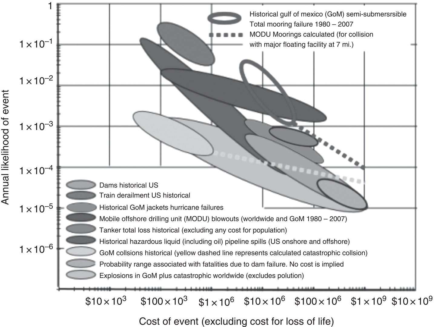
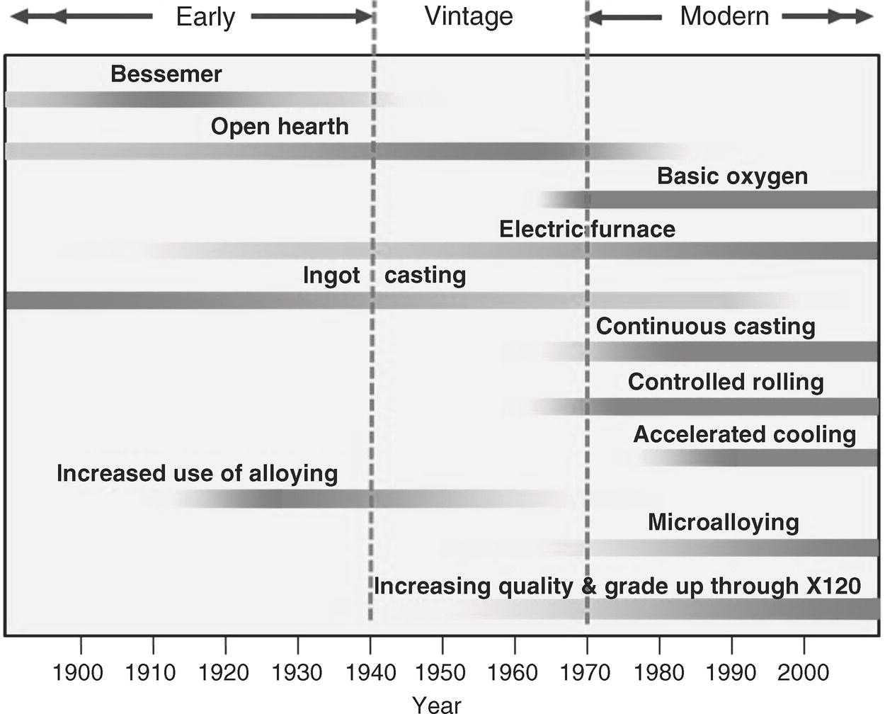
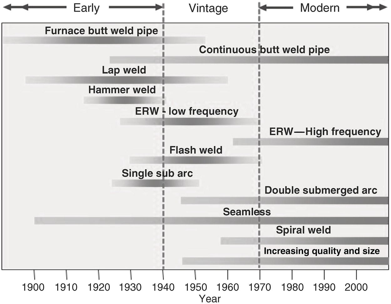
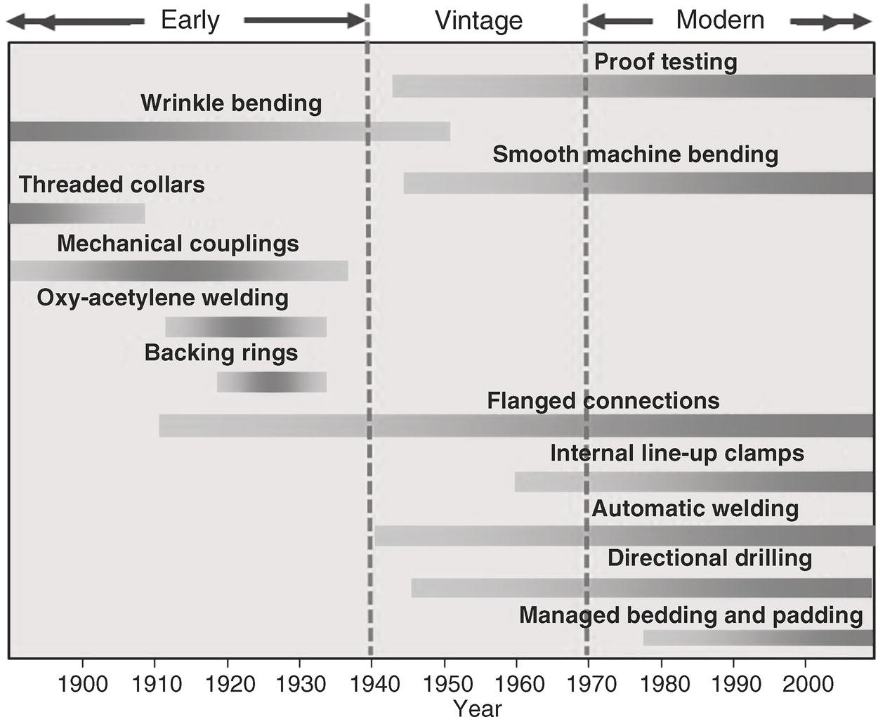
41.3 Evolution of Linepipe Steel, Pipe Making, and Pipeline Construction
41.4 Pipeline System Expansion and the Implications for “Older” Pipelines
41.4.1 System Expansion and Construction Era
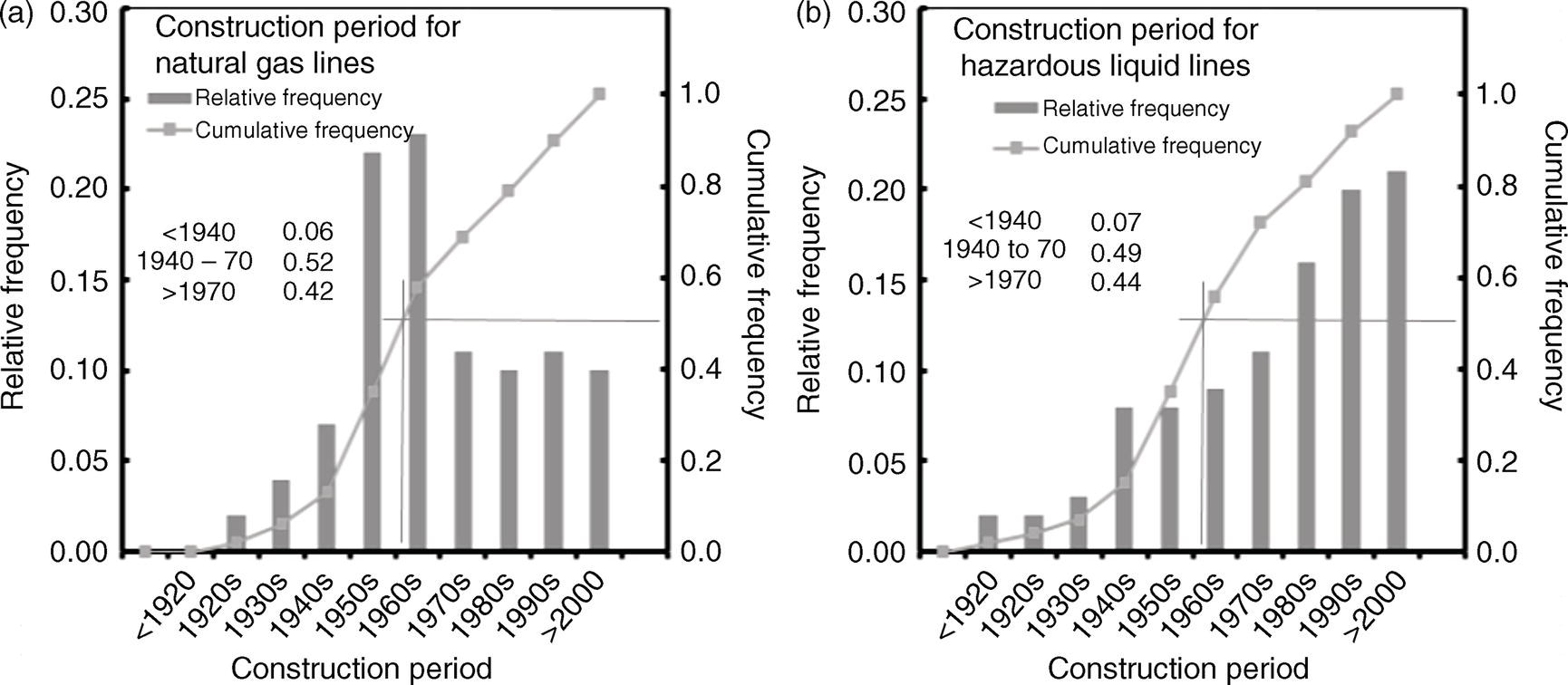
41.4.2 Qualitative Assessment of Construction Era and Incident Frequency
41.4.3 Quantitative Assessment of Construction Era and Incident Frequency
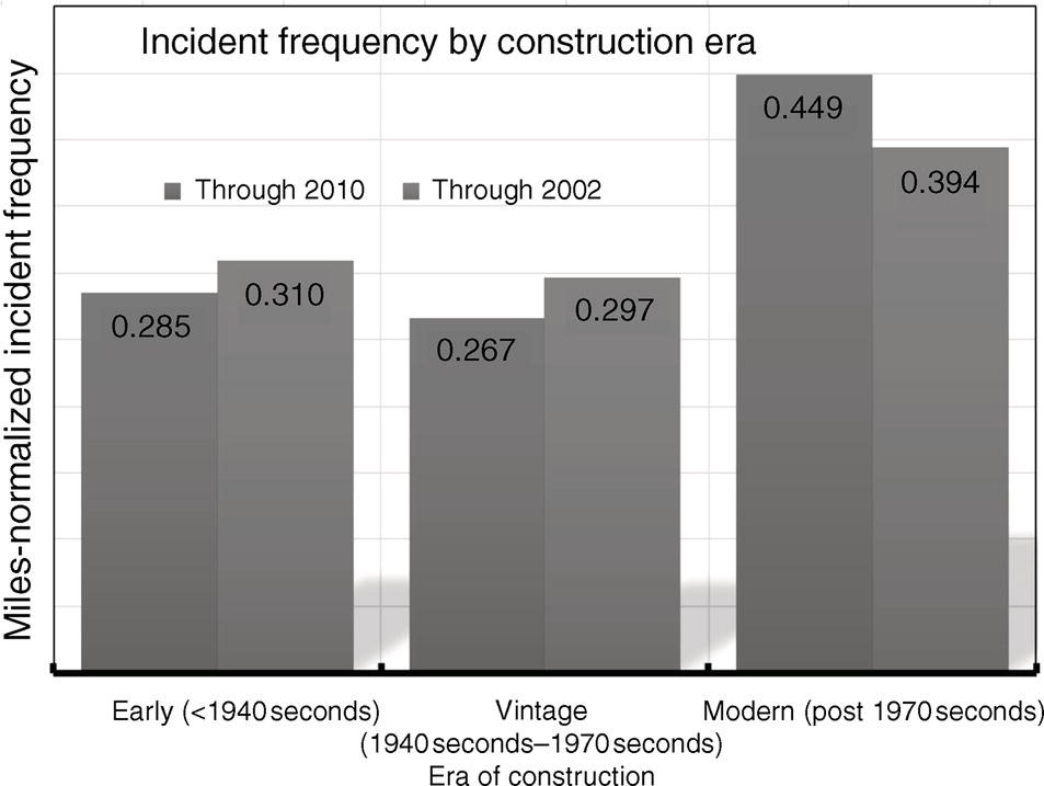
41.5 The Evolution of Pipeline Codes and Standards, and Regulations
41.5.1 Pipeline Codes and Standards
41.5.2 Pipeline Regulations
41.6 Some Unique Aspects of Early and Vintage Pipelines
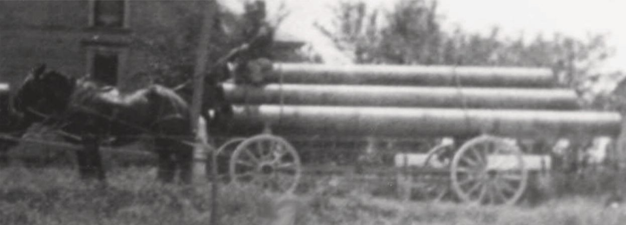
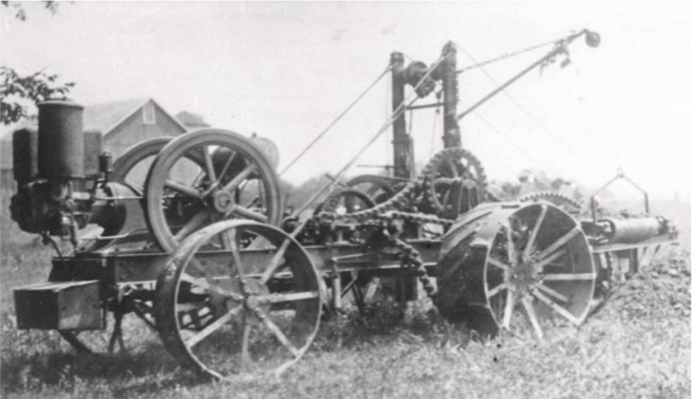
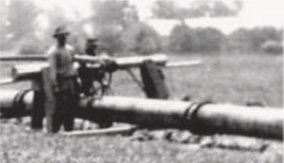
41.6.1 “Early” Construction Practices
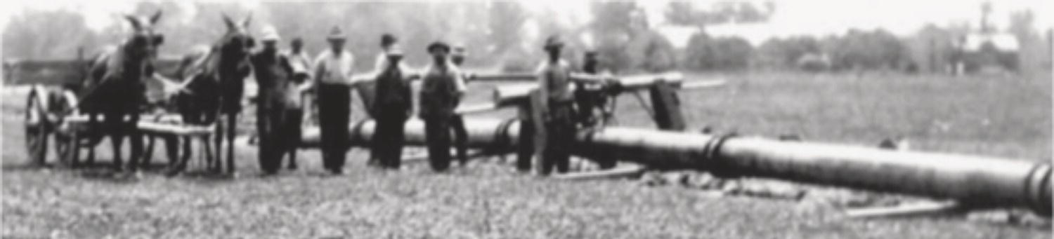
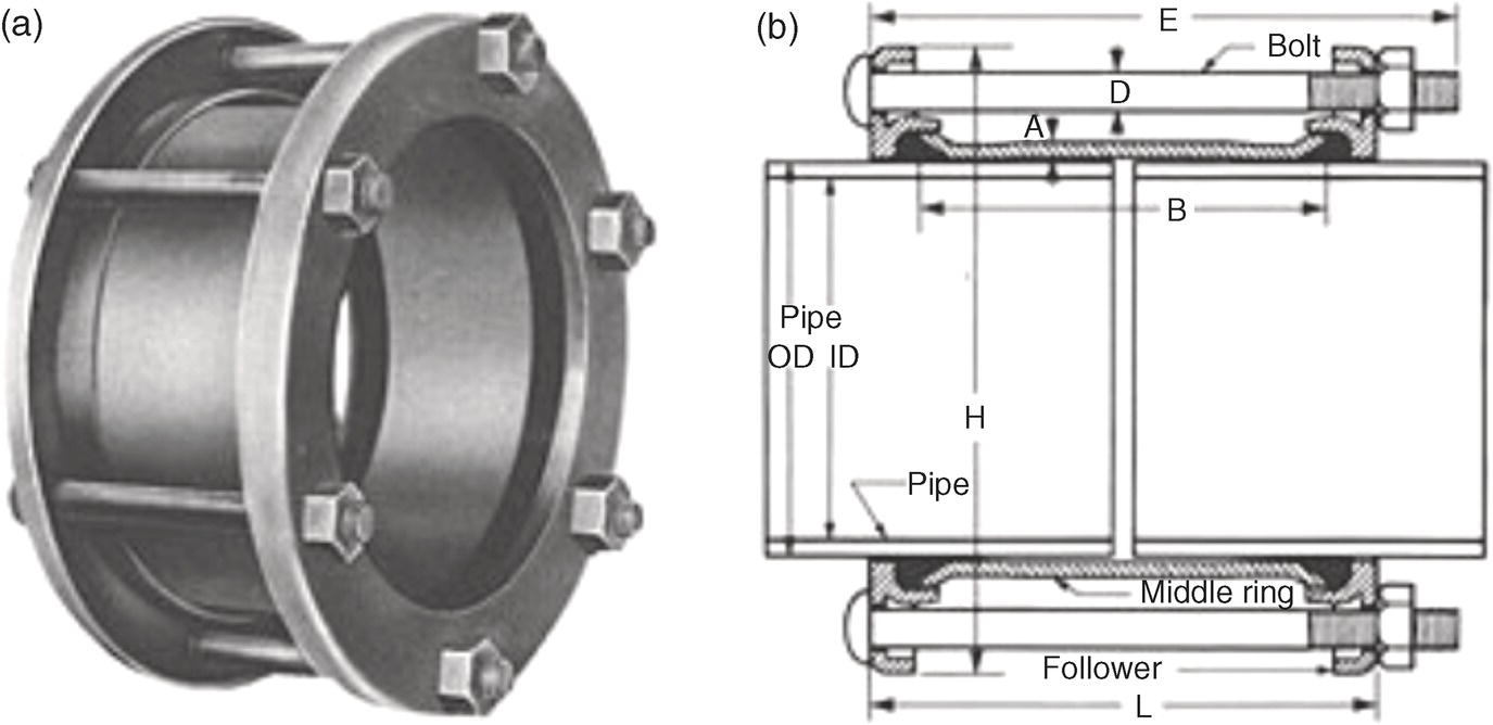

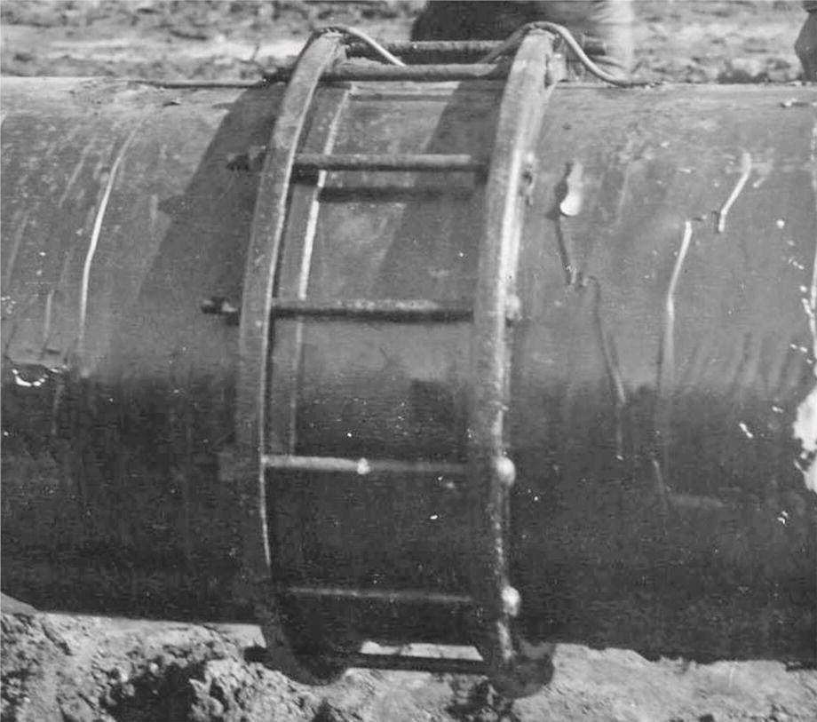
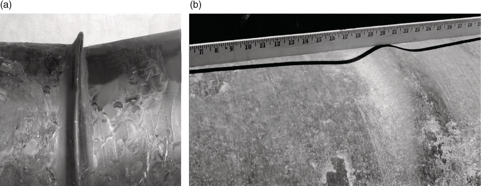
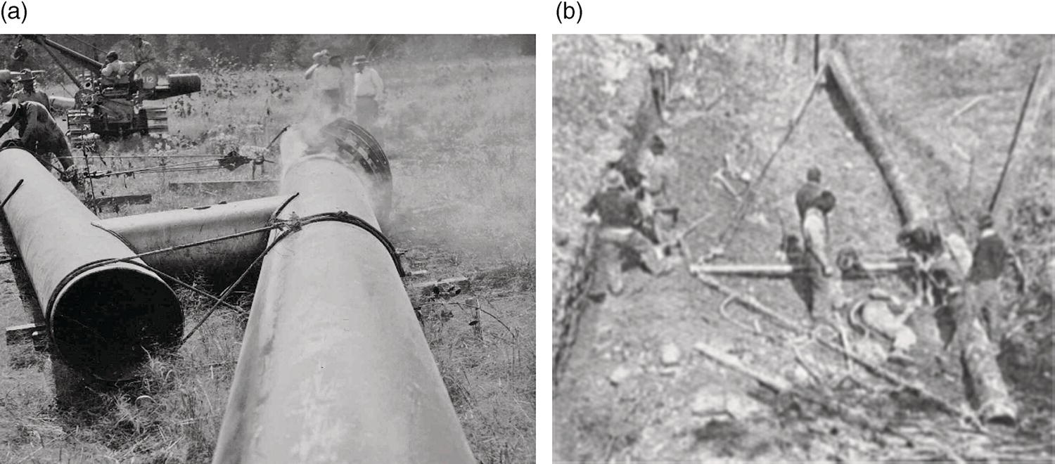
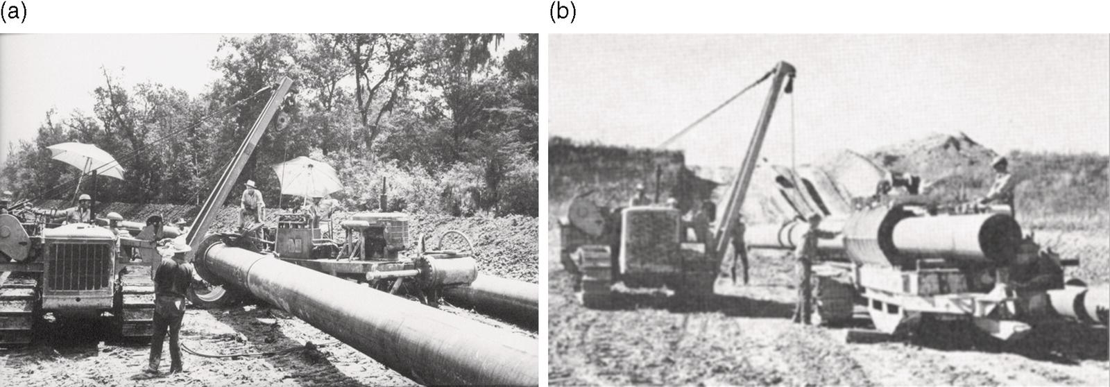
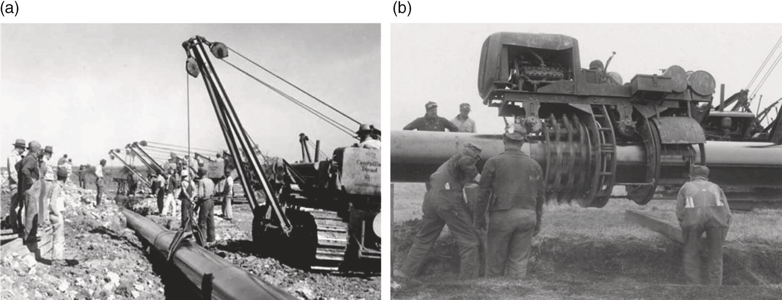
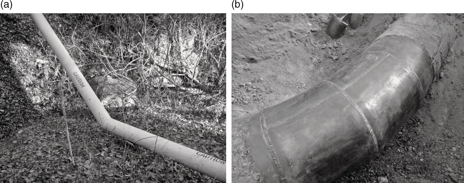
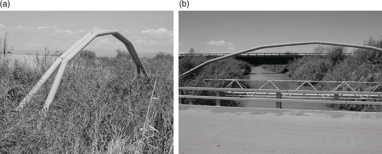
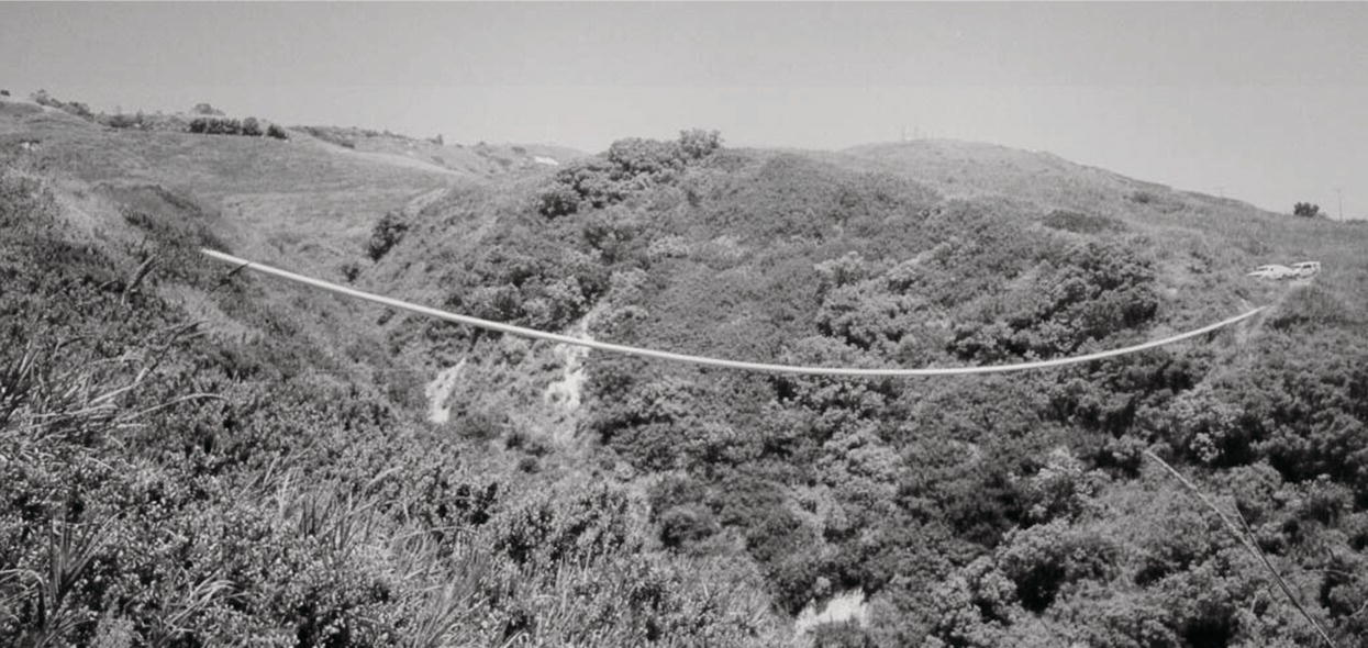
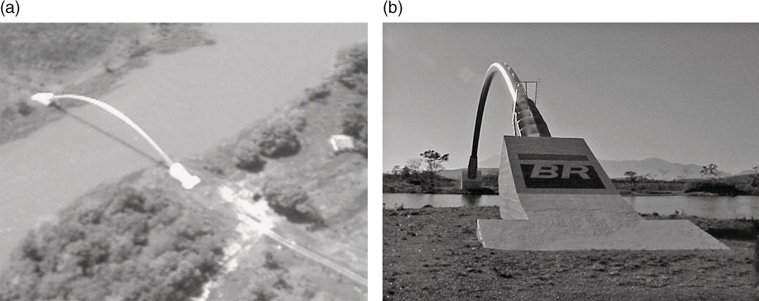
41.6.2 “Vintage” Construction Practices—An Era of Change
41.6.3 Summary and a Brief Look Forward at the “Modern” Construction Era
41.7 Management Approach and Challenges
41.7.1 Threat Identification and Assessment
Time Dependent
Stable
Time Independent
External corrosion
Materials (manufacturing)
Excavation (third-party/mechanical damage)
Internal corrosion
Construction (welding and fabrication)
Hydraulic event (incorrect operations)
Stress corrosion cracking
Equipment
Natural hazards (heavy rains/floods, earth movement)
41.7.2 Inspection and Condition Monitoring
41.7.3 Life-Cycle Management
41.8 Closure
Acknowledgments
References
Notes