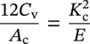
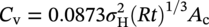
William Tyson CanmetMATERIALS, Natural Resources Canada, Hamilton, Ontario, Canada “Fracture control” has as its objective the prevention of leaks and ruptures caused by crack growth. There are many conditions that can lead to loss of containment, including various mechanisms for flaw initiation and growth such as fatigue and stress corrosion cracking (SCC), and material loss by corrosion and subsequent rupture. Failure by growth of a dominant crack is controlled by the applied crack driving force and the material resistance. Final failure may be by unstable growth of the crack or by overload tensile failure such as occurs to terminate a tensile test. Methods to assess flaws are dealt with by Ted Anderson in Chapter 35 of this Handbook. The important subject of prevention of failure by material loss through general corrosion warrants separate treatment, beyond the scope of this chapter. Much effort has been expended in deriving equations to predict the failure pressure of pipe as a function of the geometry of corroded areas. Much of this work is based on finite element analysis (FEA) parameterized in the form of equations for practical use, taking into account the geometry of the pipe and flaw and the tensile properties of the pipe steel. Popular references including practical procedures to characterize the shape of the corroded area and determine the maximum allowable operating pressure (although based on semiempirical relationships rather than FEA) are ASME B31G [1] and RSTRENG [2]; Zhu and Leis [3] have reviewed and evaluated the commonly used and three new proposed criteria, and a summary has recently been published by Qin and Cheng [4]. Similarly, SCC is a separate subject discussed in Chapters 30 and 31. In addition, practical approaches to SCC including prevention, investigation, management, and mitigation may be found in a document by CEPA (Canadian Energy Pipeline Association) [5]. Failure originating from dents and gouges, also a special topic, will also not be discussed here; an extensive treatment of this subject can be found in Ref. [6], a database in Ref. [7], and a brief discussion in Chapter 56 of this Handbook. The scope of this chapter is limited to fracture prevention by material selection and design, focusing on the general principles involved. Details of the steps to be followed to ensure fracture control can be found in the relevant sections of applicable pipeline standards, for example, CSA Z662, “Oil and Gas Pipeline Systems” [8]. Crack growth typically occurs through several stages. A crack may develop from an initial flaw in a weld (e.g., lack of fusion or hydrogen crack), by fatigue from a site of stress concentration (e.g., at the toe of a weld), or by environmental attack (e.g., stress corrosion cracking). When stress is applied, the flaw initially blunts by plastic flow at its tip. The region of intense plastic flow and associated material damage at the crack tip is called the “process zone.” In the process zone, voids may grow in response to hydrostatic (triaxial) stresses and microcracks may form at hard spots. Eventually, the blunted crack tip sharpens by linking with damaged regions in the process zone and growth may occur by micromechanisms characterized as ductile (microvoid coalescence) or brittle (cleavage). Brittle fracture characteristically occurs suddenly, sometimes at relatively low applied stress when the bulk of the structure remains elastic, and can lead to a catastrophe. Ductile fracture occurs more gradually, generally requiring an increase in applied crack driving force to extend the crack.1 However, rapid ductile propagation can occur if a point of instability is passed; this occurs when the rate of increase of material resistance with crack growth (the slope of the R-curve) is lower than the rate of increase of crack driving force. Fracture control has traditionally been categorized as “initiation control” and “propagation control.” The distinction is becoming somewhat blurred for modern steels that are designed for high strength and toughness. These materials generally show at least some “R-curve behavior” in which initiation is a gradual continuous process, and the early stages of growth could be termed “propagation,” although this generally occurs in a controlled fashion. In this chapter, “initiation control” refers to design and material selection to limit the extension of a flaw to a small amount, such as 0.2 or 0.5 mm beyond the initial flaw size, and “propagation control” refers to prevention of fast-running fractures that can extend over many pipe sections. This distinction is related to the concept of “leak before break” or “leak versus rupture.” The idea contained in these terms is that it is much better to design for containment of a failure within a short distance,2 thereby limiting the rate of release of fluid, than for the possibility of a long-running crack that could be catastrophic. This is possible if the fluid pressure to cause loss of containment by a flaw of a given length breaking through the wall (producing a leak) is less than the pressure required to extend the flaw along the pipe (producing a break). This is a plausible approach, and early work was focused on achieving “leak before break” conditions. Much of this work was done at the Battelle Memorial Institute in Columbus, OH, where Maxey and his coworkers pioneered the application of fracture mechanics to pipeline fracture control. The seminal document in the field was presented at the Fifth Symposium on Line Pipe Research in 1974 [10]. The equation in Figure 8.1 is the classic “ln sec” relation relating failure stress to toughness and flaw size for through-thickness cracks. It was developed from the “strip yield” model of Dugdale–Bilby–Cottrell–Swinden described in textbooks on fracture mechanics (see, for example, [10]). It has the property of describing brittle fracture in the limit of low toughness (in which failure stress depends on toughness) and “flow-stress-dependent” fracture in the limit of high toughness (in which failure stress depends on material strength). The equation was modified by Maxey and co-workers so that it could be used for surface flaws as well as through-wall flaws. To evaluate the material toughness, Maxey proposed that Kc be related to the Charpy absorbed energy Cv (the “Charpy” test is discussed in Section 8.4.1) through Equation (8.1): Figure 8.1 The “ln sec” equation of Maxey and coworkers for a through-wall flaw. The “Folias” correction is MT ≈ (1 + 1.255c2/(Rt) − 0.0135c4/(R2t2))1/2. (Adapted from Ref. [10].) where Cv is the Charpy shelf energy in ft lb, Ac is the area of fracture surface of a Charpy V-notch specimen (in2), Kc is the toughness (psi in1/2), and E is Young’s modulus (psi). (The factor 12 is introduced simply to convert ft lb into in lb for consistency of the units.) Equation (8.1) was an important step forward because it gave a simple method to estimate Kc using a parameter (Charpy shelf energy) that is widely specified and used in the pipeline industry. Although the test uses a relatively blunt notch and is performed in impact and is then applied to predict the behavior of sharp flaws under slow loading, the simple “ln sec” equation with Equation (8.1) for the toughness parameter has proven to be remarkably robust, at least for the relatively low-strength and low-toughness steels available at the time Maxey and co-workers carried out their work. The “ln sec” equation demonstrates an early form of two-parameter fracture mechanics in which failure by crack growth is controlled by a toughness parameter Kc and plastic collapse is controlled by a strength parameter Similarly, current methodologies for “stress-based design” are based on two-parameter fracture mechanics. In stress-based design, structural integrity is ensured for applied hoop stresses that are designed to remain below the yield stress including a safety factor. This is achieved by ensuring that the driving force on the largest flaw in the pipe remains smaller than the material toughness, and that the stress on the net section containing the flaw remains smaller than the plastic collapse stress. The “failure assessment curve” (FAC) in the “failure assessment diagram” (FAD) shown in Figure 8.2 appears in several structural integrity standards, notably the UK-based fitness-for-service standard BS 7910 [11] and API 579 [12]. Structural integrity is assured by confirming that the assessment point plotted at Kr = Ke/Kc (the ratio of the applied elastic stress intensity factor to the toughness) and Lr = σ/σpc (the ratio of the applied stress to the collapse stress) falls within the FAC. Kr is often calculated as (δe/δ)1/2, where δ is the crack tip opening displacement (CTOD), and Lr is often calculated as σref/σy, where σref is a reference stress and σy is the yield stress. Note that the shape of the FAC reflects the fact that the elastic-plastic crack driving force increases with increasing stress more rapidly than the elastic crack driving force Ke (i.e., Kr falls below unity as Lr increases). Also, there is actually some load-bearing capacity above the cutoff at Lr = σf/σy, where σf is the flow stress (the average of the yield and ultimate strengths) so that the FAC does not drop to zero above the cutoff. In practice, the FAD is often used to generate curves of allowable flaw size for a given design stress, displayed as length versus height, which can be used to assess detected flaws. It must be remembered in this case, however, that adequate safety factors must be applied. Figure 8.2 Failure assessment diagram for stress-based design. It is sometimes necessary to construct pipelines through unstable terrain where there is risk of substantial deformation of the pipe because of soil movement. This could subject the pipe to stresses above the yield strength. To deal with such situations, “strain-based design” (SBD) has been developed. Obviously, SBD requires exceptional toughness to withstand crack growth in the plastic strain field at large stresses. The fundamental principle, as in stress-based design, is to ensure that any crack growth is within acceptable limits and that the load-bearing capacity of the net section is not exceeded. To achieve this objective, extensive FEA calculations have been performed to enable estimation of the crack driving force as a function of flaw geometry, material properties, and applied strain. Guidance may be found in Clause 11.8.6 of CSA Z662 [8] and in DNV RP-F108 [13]. The R6 fitness-for-purpose code [14] also contains an SBD procedure, formulated in a similar fashion to the FAD. It is also necessary to measure or estimate the material resistance (toughness) under the constraints appropriate to field conditions. Conventional toughness tests subject the material to the highest possible constraint3 to generate a conservative result, but such conservatism may make SBD uneconomic. In response, test methods to generate more appropriate toughness measures have been developed. This will be discussed in Section 8.4.2. If an axial crack begins to run in a pipeline, it could travel a considerable distance if the toughness is not sufficient to arrest it. This is of greater concern for pipelines carrying gas rather than oil because the latter has low compressibility and pressure is relieved rapidly at a breach. Brittle fracture is the most dangerous mode of this type, and pipeline standards contain provisions to guard against brittle fracture in the form of requirements that the fracture appearance of full-scale specimens of pipe fractured in impact (drop weight tear test (DWTT), see Section 8.4.1) should be ductile. However, even if the fracture is 100% ductile, it is still possible for fast-running fractures to occur. Estimation of the toughness required to arrest a running crack is an important consideration in pipeline design. Figure 8.3 Stress required to propagate a crack through pipe steel (“fracture”) and that provided by the gas pressure (“gas”) as a function of velocity of the crack and of the escaping gas. (Adapted from Ref. [10].) The pioneering work of the Battelle Columbus labs in this area has stood the test of time and attests to the insightful engineering intuition of Maxey and his coworkers. Figure 8.3, adapted from the NG18 report mentioned earlier [10], shows the main features of what is now referred to as the “Battelle two-curve model” (BTCM, or TCM). The velocity of the running crack is determined by a balance between the resistance (the “fracture” curve) and the driving force (the “gas” curve). The “fracture” curve is a property of the material, and moves up or down on the stress axis for steels of higher or lower toughness. This curve shows that the stress for fracture rises as the crack velocity increases. The curve rises sharply when the inertial forces needed to accelerate the material ahead of the crack in the process zone from rest to the displacement required for fracture become large. This typically occurs, for pipe steel, at a velocity of several hundred m/s (recall that 1 ft = 0.305 m and 1 ksi = 6.895 MPa). (In comparison, brittle fracture by cleavage, requiring only small displacements in the process zone, can occur at several thousand m/s.) As the crack propagates, the stress driving the crack drops from the operating hoop stress level before fracture to a value dependent on the speed of the gas escaping from the open rupture. As understood intuitively, the velocity of the escaping gas decreases as the pressure decreases. The velocity of a decompression wave depends on the gas density, which in turn depends on the gas pressure (that can be converted directly into the hoop stress on the pipe), and the BTCM models the rupture process as a “race” between the fracture front and the decompression wave. If the toughness is low, the “fracture” curve may fall below the “gas” curve and consequently intersect it at two points. The lower stress point is unstable because for an increase in velocity the gas pressure rises faster than the resistance. Following the same reasoning, the higher stress intersection is stable, and hence the crack can run freely. However, if the toughness is high enough, the resistance lies above the driving force curve for all velocities and the crack cannot propagate. Estimation of the toughness required for arrest has been the objective of a number of programs throughout the world [15]. Maxey, based on his model for initiation (Figure 8.1) and the relation between Charpy absorbed energy Cv and toughness, proposed that the arrest toughness would correspond to a certain value of Cv. This value would depend on the gas characteristics and pipeline design parameters (pressure, diameter, etc.). The shape of the so-called J-curve (the “fracture” curve in Figure 8.3, not to be confused with the J-integral of Section 8.4.2) was semiempirically determined to rise in proportion to the sixth power of the velocity. The “gas” curve was developed using a model for isentropic (adiabatic) expansion of an ideal gas. Based on the knowledge then available of these characteristics, computer models were developed and run to generate toughness values required for arrest in pipe carrying “lean gas” (essentially methane) using pipe steel current at the time (X52–X65, with CVN absorbed energy Cv of 100 J or less). The critical arrest toughness for buried pipelines could be fitted to the following equation: where the units are Cv (ft lb), σH (ksi), R and t (in), and Ac (in2). This formula has demonstrated its utility for materials within the limits for which it was calibrated. Other groups around the world have proposed semiempirical formulas of the same general form. For example, in CSA ([8], Clause 5.2.2.3) an equation that can be used for buried pipelines and lean gas is given by where Cv is the full-size CVN absorbed energy (J), S is the operating stress or gas pressure test hoop stress (MPa), and D is the pipe diameter (mm). This relation is the “AISI” (American Iron and Steel Institute) formula, one of several similar equations developed from numerous burst tests carried out in the 1960s and 1970s. The broad similarity between Equations (8.2) and (8.3) is evident. It should be noted, however, that these equations have limited scope and should not be used for materials and fluids outside of the range for which the equations were calibrated. For example, in many current projects, the fluid being transported is rich gas with characteristics more complicated than the ideal gas depicted in Figure 8.3, and the “gas” curve is therefore different and is often estimated using GASDECOM (see [16]). Stages in the evolution of ductile fracture control methods since the introduction of the BTCM have been well described by Zhu and Leis [17] and Zhu [18]. Full-scale burst testing is still necessary today to demonstrate inherent crack arrestability. New steels with improved strength and toughness are continually being developed and used at higher stress (pressure) levels, and it has been found that the conventional formulas such as Equations (8.2) and (8.3) are progressively non-conservative as pipe grades and gas pressures increase. “Fudge factors” to adjust (increase) the required Charpy energies have been used successfully for grades up to X80, for lack of a better validated approach to toughness measurement. The Charpy test is convenient and familiar, has a well-earned role as a means to demonstrate fracture resistance, and will continue to be used in specifications. However, it is limited in several respects. The thickness of a Charpy specimen is frequently less than the pipe wall thickness and so does not develop the full constraint of a crack in a pipe. Also, for high-toughness steels much of the Charpy energy is absorbed in crack initiation rather than propagation. Indeed, for some new steels the specimen bends and does not break completely during the test, raising serious doubts about whether the test characterizes crack propagation meaningfully. The short crack path in the Charpy specimen does not allow the crack to develop fully into the form it would have in a full-scale pipe, implying that even if the propagation energy is extracted from the Charpy test, it does not characterize the same morphology as a full-scale running fracture. For these reasons, alternatives to the Charpy test have been intensively developed over the past few decades. In particular, the DWTT [19] has been assessed for use because the DWTT specimen is of full pipe wall thickness and has a crack path long enough to enable development of the same morphology as in a full-scale pipe. Also, to focus on crack propagation rather than initiation, the crack tip opening angle (CTOA) is being studied as a parameter that is much more appropriate for characterizing the propagation toughness compared with the Charpy absorbed energy. However, CTOA methods have not yet been developed sufficiently to confidently predict the arrest toughness for the full range of modern pipelines, hence the need for more full-scale burst tests. Finite element calculation methods are being developed to take into account the fluid-structure interaction (FSI) as well as the effect of backfill [20]. An ASTM standard for measurement of CTOA has been published [21] as well as an FEA procedure for prediction of CTOA requirements [22]. “Toughness” may be broadly defined as the ability of a material to absorb energy during fracture. Good toughness is an essential component of fracture control to ensure that should failure occur it will be progressive and not catastrophic. “Notch toughness” is the most familiar characterization, and refers to the energy-absorbing capacity of a specimen with a notch. It is commonly measured using the Charpy test (see Section 8.4.1) as the absorbed energy Cv. Its major use is to identify materials that are susceptible to brittle (low-energy-absorbing) fracture through characterization of a brittle-to-ductile transition temperature. Early fracture control plans, a typical example being the methodology developed by Pellini and his coworkers at the Naval Research Labs in the United States, were designed to avoid brittle fracture by ensuring that the critical parts of the structure of interest operate above the transition temperature. Although this approach has been largely superseded by quantitative fracture mechanics, the reality of the ductile-to-brittle transition phenomenon in structural steels and the practical utility of the notch toughness test will ensure the continued use of the Charpy test. For example, standards for line pipe (e.g., CSA Z245.1 [23]) routinely specify notch toughness as a requirement. Another important characteristic of Charpy data is the “upper shelf” absorbed energy, used to characterize the resistance to ductile fracture, although caution is required in interpreting this value for high-toughness steels for which the Charpy specimens may not actually break in two. “Fracture toughness” characterizes the resistance to propagation of a sharp crack. It can be quantified in a number of ways. The earliest to be used was the “plane strain fracture toughness” KIc (see test standard ASTM E399 [24]), defined as the stress intensity factor at fracture initiation and primarily elastic conditions, that is, where the plastic zone at the crack tip is much smaller than the specimen size. However, if fracture does occur under such “small-scale yielding” conditions, the material would be completely unsuitable for a pipeline, and so E399 is irrelevant for pipe steel. Rather, “elastic-plastic fracture mechanics” has evolved to address the need for toughness parameters and tests involving substantial plasticity. The associated parameters are the J-integral and the CTOD, defined and discussed at length in standard textbooks (see, for example, [9]). The CTOA is another elastic-plastic parameter to characterize propagating cracks, and has been standardized by ASTM for sheet material [25] and for plate [21]. The Charpy test (ASTM E23 [26]) was standardized in the early 1900s. The full-size Charpy specimen is a small bar, dimensions 55 × 10 × 10 mm3, with a 2 mm deep notch in the center. The specimen is fractured in impact, usually in a pendulum machine, and the absorbed energy Cv is measured. Line pipe specifications normally require a certain absorbed energy at a specified temperature related to the pipeline design temperature. The test is often used to identify a ductile-to-brittle transition temperature (DBTT), defined as the temperature at which the value of Cv is equal to some predetermined value in the transition range or the temperature at which the cleavage portion of the fracture surface reaches a specified fraction (often 50%, but in the pipeline industry 85% is required for DWTT tests). Typical CVN transition curves are shown in Figure 8.4 for a high-strength pipe steel and its weldment. The DWTT (API RP 5L3 [27] or ASTM E436 [19]) uses a significantly larger specimen of full pipe wall thickness and in-plane dimensions of 3 × 12 in.2 (76 × 305 mm2). The specimen is placed in either a drop tower or pendulum machine and impacted at a velocity no less than 4.88 m/s. The shear area fraction is measured on the fracture surface, and should be at least 85% to ensure that a fracture running in the pipe will propagate primarily by a ductile mode. With the increasing sophistication of mill test labs, there is growing interest in instrumenting the test to enable measurement of load and displacement to give absorbed energy and its components (initiation and propagation) and the steady-state CTOA, using DWTT specimens. This should give a much more realistic quantification of the full-scale propagation resistance than can be obtained using Charpy specimens. Figure 8.4 Typical Charpy test results, for high-strength steel X100 and weldment 807-F, showing results for pipe (base metal), HAZ-FL (heat-affected zone, notch centered on the fusion line), and weld metal WMC (weld metal centerline: specimen extracted in either root region or cap region). (Adapted from Ref. [33].) Fracture mechanics has provided quantitative tools to describe crack phenomena. The practical importance of this for the design of pipelines is that the significance of flaws, notably imperfections in girth welds, can be quantitatively assessed by engineering critical assessment (ECA) using methods such as those described in Section 8.2 and in Chapter 63 of this Handbook. Also, steady advances are being made in the control of fast ductile fracture using the CTOA. Flaws can grow by micromechanisms that may be either brittle (cleavage or intergranular fracture) or ductile (microvoid coalescence). The latter is clearly preferable, as brittle fracture can be catastrophic. However, even ductile fracture can lead to unstable propagation, and it is important to characterize the resistance to fracture by either the J-integral or CTOD. Either of these parameters is sufficient to quantify the driving force. The CTOD was championed by researchers in the United Kingdom, and the British standard [28] remains in popular use in the pipeline industry. ASTM was the first to standardize J-integral testing, and ASTM E1820 [29] remains preeminent in many industries in North America. Increasing globalization has led to pressures to consolidate (“harmonize”) standards, and the International Organization for Standardization now has toughness test standards for homogeneous materials [30] and for welds [31]. ASTM standards for toughness testing have been summarized by Zhu and Joyce [34]. The basic methodology in elastic-plastic fracture mechanics testing involves loading a precracked standard specimen, the most popular in the pipeline industry being a three-point bend bar, and measuring the crack size as a function of the applied force. In the most commonly used procedure, the specimen is instrumented to measure the crack mouth opening displacement (CMOD), which enables calculation of the J-integral and CTOD using equations developed with the use of FEA. The specimen is periodically subjected to unload-reload cycles to measure the CMOD compliance and thereby calculate the crack size from established relations between the compliance and the crack size. In earlier standards, the CTOD was estimated using a model in which the specimen was idealized as rotating about a plastic hinge in the ligament, but the current trend is to evaluate CTOD directly from the J-integral using correlations developed using FEA. Unfortunately, the two methods do not agree in all cases, and this raises the issue of the use of CTOD-from-J in ECA procedures that were validated using CTOD toughness measured with the older standards. If the older methods gave lower values of CTOD, the ECA procedure could be non-conservative with the use of current measures of CTOD. This issue remains to be resolved. A three-point bend bar generates significant triaxial stresses (i.e., high constraint) at the crack tip, and intentionally provides lower bound estimates of the toughness. With current trends to use higher strength steels designed to withstand plastic strains in service, the lower bound estimates may be excessively conservative. It is important to provide toughness data that are relevant to the service conditions. Pipe steel is relatively thin-walled compared with other engineering structures. It is difficult to generate high triaxiality in thin structures, especially if plastic yielding occurs, and so the constraint is significantly lower (and the toughness higher) for cracks in pipe than for cracks in highly constrained test specimens. The low-constraint toughness can be higher than the high-constraint toughness by a factor of the order of 2 for shallow cracks. Consequently, there has been considerable interest in developing a low-constraint test that simulates service conditions more closely. Det Norske Veritas (DNV) was the first to standardize such a test [13] using a single-edge-notched tensile (SE(T) or SENT) specimen loaded in tension. The DNV test requires at least six specimens to develop an R-curve, but single-specimen procedures have now been standardized [32]. Some typical J–R curves measured using a single-specimen test procedure are shown in Figure 8.5. Figure 8.5 Typical low-constraint SE(T) J–R curves for a high-strength steel weldment: BM (base metal), WM (weld metal), and HAZ (heat-affected zone), measured using shallow-cracked (a/W = 0.17) single-edge tension specimens at −20 °C: R1 and R2 denote two rounds of nominally identical X100 steels and welds. (Reference [33]/American Society of Mechanical Engineers.) For resistance to fast fracture, the first objective is to ensure that the fracture occurs by a ductile mechanism. Current line pipe standards specify that the fracture mode should be primarily shear in full-wall-thickness specimens tested in impact using the DWTT (e.g., 8). The second objective is to ensure an adequate level of toughness. As related in Section 8.3, current standards characterize the energy-absorbing capacity of a pipe steel using the Charpy test. This is well known to overestimate the resistance for high-strength steels, and as noted in Section 8.4.1, current efforts are under way to use the CTOA as a suitable alternative parameter. As described above, ASTM E3039 is now available for measuring CTOA. Fracture control for stress-based design (with operating stresses below the yield stress) is well understood. Pipeline standards include procedures to guard against rupture at locations where the pipe wall has thinned owing to general corrosion, and methods are available including inspection and remediation to combat stress corrosion cracking. Fracture mechanics methods have been developed to assess fitness for service in the presence of flaws, enabling evaluation of weld imperfections. Suitable test standards to measure material toughness are in general usage. The state of the art in practical approaches to fracture control as of 2008 was well summarized by Widenmaier and Rothwell [15]. The primary objective incorporated in existing standards is the avoidance of brittle fracture. Although modern steels are being produced with increasing strength and design stresses are increasing accordingly, these steels can also be made with excellent toughness and so brittle fracture in the pipe body is normally not a concern. However, during welding the carefully designed finegrained microstructure is changed and some regions of the HAZ can have a coarse-grained structure of low toughness. Care must be taken to ensure that the toughness properties of the weld are well characterized and that flaw acceptance standards recognize the possible presence of low-toughness regions in welds. Prevention of fracture propagation in the form of fast-running ductile rupture can be achieved automatically for oil lines (because of the low compressibility of oil) and for gas lines using the two-curve method for “normal” pipeline designs using steels of modest strength and toughness and lean gas. However, for demanding situations of highly stressed high-strength pipe and possibly rich gas, traditional methods have been shown to be inadequate and special measures must be taken to guard against running ductile fracture. Methods of design and material specification to achieve this based on CTOA are under development.
8
Material Selection for Fracture Control*
8.1 Overview of Fracture Control
8.2 Toughness Requirements: Initiation
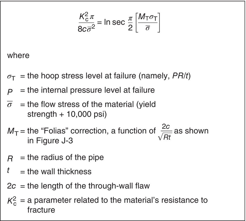
 . In the toughness-dependent limit, the “ln sec” equation in Figure 8.1 reduces to
 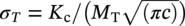 . In fracture mechanics terms, this states that the crack driving force (stress intensity factor
 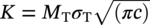 ) is equal to the material toughness Kc. Similarly, in the flow-stress-dependent limit
  , which states that the concentrated hoop stress MTσT is equal to the material flow stress
  . Note that the “Folias factor” MT, which increases with the variable
  , acts as a stress concentration factor that amplifies the hoop stress by the action of the fluid pressure to cause bulging at the crack tips.

8.3 Toughness Requirements: Propagation

8.4 Toughness Measurement
8.4.1 Toughness Measurement: Impact Tests
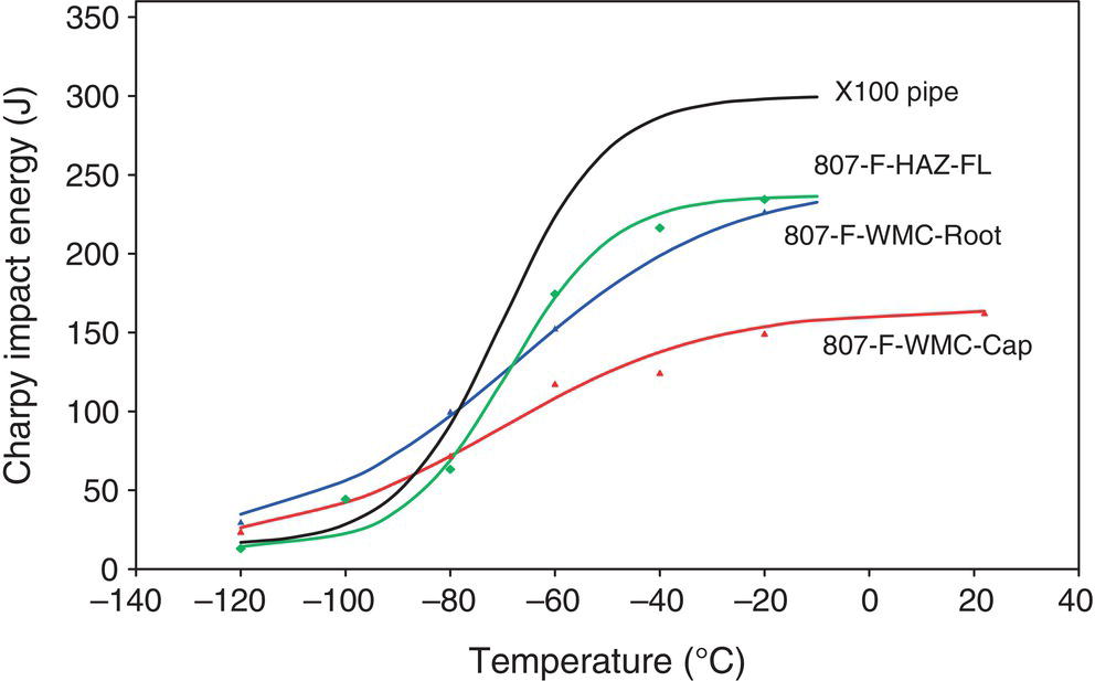
8.4.2 Toughness Measurement: J, CTOD, and CTOA
8.5 Current Status
References
Notes