Ming Gao* and Ravi Krishnamurthy Blade Energy Partners, Houston, TX, USA Pipelines can be mechanically damaged by external force from third-party intrusion, contact with rocks in the backfill, or by settlement onto rocks. Mechanical damage typically includes pipe coating damage, dent(s) in the pipe, and gouge(s), all localized or confined to some portion of the pipe along the pipe’s length. A majority of the anomalies caused by outside forces do not have dire consequences. However, a few prominent pipeline failures have been attributed to mechanical damage [3]. While dents are common, failures from plain dents alone without additional surface mechanical damage such as gouges and cracks are relatively rare. Dents with additional surface mechanical damage resulted in immediate failure at approximately 80% of the time [4]. In the remainder of mechanical damage events, damage was not severe enough to cause immediate failure. However, delayed failure is feasible, if the internal pressure is increased sufficiently, or if corrosion or cracking develops in the damaged material, or if there is pressure-cycle fatigue. Table 57.1 shows the total number of reportable incidents in the United States from all cases and the number of incidents from mechanical damage in a total of 460,000 miles of gas and liquid pipelines from 1985 through 2003. Statistical data showed that mechanical damage is one of the major threats for pipeline integrity. As illustrated in Figure 57.1, 33.7% of serious incidents on all types of pipelines from 1994 to 2013 were caused by mechanical damage during excavation, which is more than by any other single cause [5]. Excavation damage continues to be a leading cause of pipeline incidents. Pipeline incidents caused by excavation damage can result in fatalities and injuries, as well as significant costs, property damage, environmental damage, and unintentional fire or explosions. Significant efforts have been made over the past 30 years by the Office of Pipeline Safety (OPS) and now Pipeline Hazardous Material Safety Administration (PHMSA) of U.S. Department of Transportation, the pipeline industry, and stakeholder organizations with regard to the reduction of serious pipeline incidents. The efforts include (1) increased public awareness of the risks of excavation in pipeline corridors and prevention, (2) investment in research to detect mechanical damage using in-line inspection (ILI), (3) improvement in evaluation of the severity of mechanical damage, and (4) development of mitigation measures [6]. Such significant efforts have greatly reduced serious incidents over time. Since 2005, pipeline operators have reported excavation damage as the cause of 1273 incidents, (11.1% of serious incidents) about three times less than in 1994–2013. Figures 57.2 and 57.3 show the trend for serious pipeline incidents caused by excavation damage for a 20-year period from 2005 to 2023. This positive trend is the result of a broad array of initiatives at all levels designed to engage all stakeholders in efforts to reduce the risk of damage to underground facilities [5]. However, the 1273 incidents resulted in 59 fatalities, 227 injuries requiring in-patient hospitalization and $628,772,878 of property damage, showing that the consequence of serious incidents is significant. Great efforts are still required regarding the reduction of serious pipeline incidents due to excavations. In this chapter, the types of mechanical damage are summarized first. The status of in-line-inspection technologies for mechanical damage characterization, mainly dent and dent with gouge/crack, is reviewed. The improved technologies for in-ditch assessment of mechanical damage and validation of ILI tool performance are then summarized. The assessment methods of the severity of mechanical damage and associated regulatory and industry guidelines are presented. Finally, a brief review of the prevention and mitigation of mechanical damage is given. Table 57.1 Analysis of Reported Mechanical Damage Incidents in the USA Source: Adapted from Ref. [3]. Figure 57.1 1994–2013 serious incident cause breakdown, indicating 33.7% of serious incidents caused by excavation damage [5]. (PHMSA Significant Incidents Files, February 4, 2014.) Figure 57.2 2005–2023 serious incident cause breakdown, indicating 11.1% of serious incidents caused by excavation damage, about 3 times less than in 1994–2013. (DOT/PHMSA Pipeline Incident Data Ref. [6].) Figure 57.3 Serious pipeline incidents caused by excavation damage—all pipeline systems. (DOT/PHMSA Pipeline Incident Data Ref. [6].) A dent is a local inward depression in the pipe surface caused by an external force that produces pipe wall plastic deformation and a disturbance in the curvature of the pipe from its original shape. Dents are formed by the application of external concentrated force(s) to the exterior surface of the pipe. Commonly, there are three stages involved in the dent formation process [8]: Figure 57.4 Illustration of stage I—elastic ovalization of the pipe: (a) round pipe prior to the indenter contacting the pipe and (b) ovalized pipe elastically first when the indenter contacts the pipe. Figure 57.5 Illustration of stage II: indentations to form a dent. Figure 57.6 Illustration of stage III—indenter removal: the indenter removal results in a change in pipe cross-section and dent depth. Different types of dent–defect combinations that can develop on pipelines are illustrated in Figure 57.7. Based on the dent formation process, dents are commonly characterized as the following six types [8]: Figure 57.7 Schematic diagram illustrating different types of dent–defect combinations that can be present on pipelines. (Reference [9]/with permission of Elsevier.) The dent formation process may promote or result in the geometric coincidence of additional features with a dent. Examples of coincident features and their evolution include Dent with coincident features are more severe than plain dents, and engineering assessment is necessary. The fitness-for-service assessment should evaluate if the geometrically coincident feature affects the failure pressure or fatigue life and thus is interacting with the dent. Fitness-for-service procedures should incorporate the stress concentration effects of the coincident features, material inhomogeneity, changes in dent shape, and potential for coincident feature growth with time or loading. Resulting maintenance decisions and repair strategies should include the coincident feature in the dent maintenance or repair processes. It should be noted that the above dent formation process is limited to static loading. For dynamic loading, the conditions and process for dent formation and their impact on dent severity are significantly different and will be discussed in Section 57.5.5 (Dynamic-Strain Based Dent Severity Assessment) of this study. Dent integrity programs typically consist of in-line inspections, field inspections, and engineering assessments used to identify features that pose integrity concerns [12]. As dent features can often remain dormant for long periods of time, multiple inspections are often required, and their results are tracked by operators to identify any changes in condition such as changes in the shape or the generation of cracks or corrosion within the dent. Due to challenges associated with inspection and assessment (as discussed later in this paper), the integrity programs also heavily rely on historical experience and operator-specific procedures and criteria for managing this integrity threat [12]. Technologies and associated ILI tools identified as having potential for mechanical damage detection and discrimination can be categorized as one of three types: dimensional (Calipers), electromagnetic (MFL), and ultrasonic (UT, EMAT) [10–15]. Dimensional measurement technology (mainly calipers) directly measures the deviation from circular form of the pipe wall and has been used for detecting, locating, and sizing dents, wrinkles, cold bends, etc. This technology is generally regarded as providing the most accurate results for sizing dents and wrinkles at specified detection thresholds (for example, 2% OD for dents), but it is not capable of detecting other defects associated with dents such as corrosion, cracks, and gouges. Therefore, dimensional technology in conjunction with other technologies, such as ultrasonic, magnetic and/or electromagnetic technology, maybe utilized to reveal the extent and severity of mechanical damage defects. Magnetic flux leakage (MFL), both axial and circumferential fields, has been shown to be sensitive to geometric and magnetic changes due to mechanical damage and is capable of detecting some mechanical damage [16]. The magnetic signal indicating mechanical damage is driven primarily by geometric changes (local metal loss or moved metal and denting). Other parts of the signal are mainly associated with changes in magnetic properties resulting from stresses, strains, and metallurgical changes of line pipe steels. Ultrasonic technologies have also been used to detect dents and cracks. Identification of the dent by UT is feasible; however, dent sizing is inconsistent. Despite a high probability for detection of cracks in the plain pipe, the probability of detection of cracks within dents will decrease with increasing size of the dents. Sizing of cracks within dents by ILI is not feasible with any degree of reliability. Additionally, application of UT requires a liquid medium; consequently, practical operational limitations exist for application in gas pipelines. Multiple geometry ILI tools are available that can provide various levels of deformation details. These tools can generally be grouped into two categories: single-channel tools and multiple-channel tools [17]. Single-channel tools only provide the minimum pipeline diameter and distance traveled, which are useful for new construction or line segments that have never been inspected. The single-channel tools offer simple operation, low inspection cost, the ability of passing large reductions of pipe diameter, and rapid analysis of the geometrical data. However, they offer little information on orientation and geometrical profiles of the deformation that are required for performing strain and stress calculation from the results [17]. In contrast, multiple-channel ILI tools provide detailed information on orientation, length, width, maximum depth, and geometrical profile of the deformation, which can be used for deformation severity evaluation based on strain calculation. They are also reliable for locating and characterizing deformation anomalies. Therefore, a multiple-channel ILI tool is recommended for use in serving the purpose of developing an integrity management plan for mechanical damage [17]. Three types of multiple-channel geometry sensing technologies are used to detect and characterize plain dents in the pipe wall. Direct arm measurement sensing technologies are generally employed in tools known as caliper. All direct arm measurement calipers (DAMC) employ multiple mechanical arms (fingers) for dent characterization, which measure the interior of the pipe geometry by contacting the inner surface of the pipe and are often referred to as “multi-channel” calipers. Each arm is equipped with a sensor that measures the angle of the arm (such as Hall effect or eddy current transducers). These multi-channel tools provide data, such as depth, length, width, location, and orientation of the deformation. Various proprietary mechanical designs are incorporated to address issues associated with sampling intervals, inspection speed excursions, sensor bounce, vibration, and sensor coverage of the internal pipe surface. Some caliper technologies were reported to be augmented with electromagnetic (EM) sensors at the ends of the mechanical arms (Hall effect or eddy current sensors). These electromagnetic sensors, DAMC(EM), provide an additional data stream for analyses that address potential sensor liftoff, which occurs due to tool speed/sensor inertia, deformation geometry, interior cleanliness of the pipe, and other conditions. Indirect electromagnetic calipers (IEMC) were also identified for deformation measurements. This type of sensor does not rely on direct contact with the pipe wall. A ring of electromagnetic sensors (eddy current) are mounted on a fixed diameter ring, with a diameter sufficient to allow for passage of the tool through a maximum expected bore restriction and gauge the distance between the ring and pipe wall. Limited validation data were made available for this technology. Figure 57.8 is an illustration of the three types of caliper sensing technologies for detection, discrimination, and sizing of plain. The probability of detection (POD) and sizing performance for all deformation technologies are greatly influenced by the circumferential coverage of the sensing area by the caliper sensors [18]. The data sampling rate and contact area of individual sensors also affect performance. Design and spacing of the sensing arms determine the circumferential resolution of a caliper tool. Narrow arms provide greater resolution of the contour. Conventional resolution direct arm calipers are typically designed with the same number of arms as the nominal pipe size (NPS), such as 12 arms or 20 arms for NPS 12 or 20 pipelines, respectively. The circumferential spacing between the sensing arms is approximately 3.14 in. when the number of sensors equals the NPS [17]. Higher-resolution caliper tools of the types are designed with narrower spacing as small as ¾″, typically 1–2 in. Caliper tools have also been designed with paddles. Radius-tipped paddles provide more coverage of the inside surface than narrow arms, and burs tend to average the width of the deformation. Conversely, narrow arms provide greater resolution of the deformation contour but do not record deformation that passes between adjacent arm sensors. Figure 57.8 An illustration of the three types of caliper sensor technology for dent characterization. Coincident damage for the purposes of this chapter is classified as corrosion, gouges, and cracks associated with dents. Damage from gouges was broadly categorized as localized damage due to moved or removed metal [19]. Magnetic flux leakage (MFL) and ultrasonic tools (UT) in combination with deformation tools are utilized to detect and discriminate localized mechanical damage in the form of corrosion, gouge, and gouge with crack, within the deformation. The sensitivity to deformation detection depends on the type of the sensor, the size of the sensors, and the type of sensor assembly. MFL, both axial and circumferential magnetic fields, has been shown to be sensitive to geometric and magnetic changes due to mechanical damage and is capable of detecting dents and dents with metal loss [10, 16]. MFL tools do respond to any sharp portions of the deformation by the sensors “lifting off” the inside pipe surface. This creates a magnetic field change, causing a signal response. However, the signal shape for a typical MFL signal from a dent is fundamentally different than that seen from metal loss. Furthermore, the MFL signal from a cold-worked region will generally exhibit a signal shape different from that of metal loss and dent. This enables the MFL to detect and discriminate the metal loss and cold work within the dent. The proper analysis of the MFL raw data is the key to gaining information about the deformation anomalies. In all cases, except one MFL technology i.e., tri-axial MFL technology, [8, 9], analyses of mechanical damage, i.e., deformation coincident with metal loss, include integrated analysis of caliper-based deformation data in conjunction with MFL data. Generally, conventional MFL tools alone are not considered to be reliable for identifying and sizing dents, except the triaxial MFL tools. Therefore, in the majority of cases, the detection and discrimination of dents and dents with metal loss relies on the integration and analysis of multiple data streams. Often, these data originate from multiple in-line inspection tools or from tool technologies that have been mechanically combined into a single tool. For the multiple in-line inspection tools, the mechanical damage was inspected with deformation (caliper) tools and MFL tools separately. For the combined technologies, this is a single COMBO tool that ran once. For the multiple data streams, automated analysis of ILI signals from calipers and metal loss from MFL tools is known to be a normal practice for inspection vendors. However, the integration of data from multiple tools and analysis of these data streams for the purposes of mechanical damage detection and discrimination rely heavily on subject matter expert analysis and interpretation. For the tri-axial MFL technology [10], because it utilizes tri-axis Hall effect sensors along with magnetic models to incorporate both stress and geometry effects to interpret MFL signals from dents, this technology does not require a caliper data stream to characterize deformation. The performance of the tri-axial MFL tools for detecting and discriminating deformation with coincident metal loss was evaluated with limited field data [10] and is reported later in this chapter. Table 57.2 summaries these technologies in their generic category description, which are used by the pipeline industry for characterization of mechanical damage. In the table, the technologies for crack detection, UT and EMAT, are not included, but they are similar to MFL and can be combined with caliper but run separately. So far, there has been no combo type of tools for dents with crack detection tools. The capabilities and performance of mechanical damage technologies have been evaluated under a project “Investigate Fundamentals and Performance of Current Inspection Technologies for Mechanical Damage Detection” funded by the Pipeline Research Council International (PRCI) [10, 20]. Since this evaluation provided the latest and most complete information on the capabilities and performance of the current mechanical damage technologies and were validated using extensive excavation data collected from both ILI vendors and pipeline operators, the results are used in this chapter. The current deployed ILI-based technologies for detecting, discriminating, and sizing dents and dents with metal loss are summarized in Table 57.3. Clearly, geometry (caliper) ILI tools alone are capable of detecting and sizing dents but incapable of detecting and sizing metal loss in the deformation. For detecting metal loss coincident with deformation, the combined technologies, or the tri-axial MFL technology, should be used. However, their capability in discrimination of metal loss between corrosion and gouge/crack is limited by high uncertainty with low confidence, if not impossible. Table 57.2 Categorization of In-line Inspection Technologies for Mechanical Damage Characterization (Source: Reproduced from Refs. [9–11]. The full copy of the report can be found at www.prci.org, ©Pipeline Research Council International, Inc. PRCI bears no responsibility for the interpretation, utilization, or implementation of any information contained in the report.) Table 57.3 Capabilities of Current In-Line Inspection Technologies to Detect and Discriminate Dents and Dents with Metal Loss Condition The performance of any ILI technologies can be measured with the following four parameters: probability of detection (POD), probability of identification (POI), probability of false call (POFC), and sizing tolerance, in accordance with the procedures recommended by API 1163 ILI [21] and using the binomial probability distribution methods [22–24]. The following are their definitions: The method used for calculating POD, POI, POFC, and sizing tolerance are the binomial probability distribution and confidence interval methods in accordance with API 1163 [21]. For confidence interval methods, the Clopper–Pearson method known as the “Exact” confidence interval for binomial probability distribution is preferred because this confidence interval method provides the most conservative intervals, PL and PU, i.e., the lower and upper ends of the interval, respectively, for a given confidence level. The details of the binomial distribution analysis and Clopper–Pearson confidence interval methods are given elsewhere [22–24]. In the following section, the performance of current ILI technologies for characterization of dents and dents with metal loss in terms of POD, POI, POFC, and sizing tolerance is summarized and reviewed [10, 11, 20]. It is known that the probabilities of detection and identification of dents for the depth greater than 2.0% OD in pipelines are very high, and the probability of false call is very low for all types of generic technologies listed in Table 57.4. POD, POI, and POFC were not the concerns. Only the sizing performance was evaluated and reported [10, 23]. For dent sizing, geometry sensing technologies (calipers) are generally regarded as providing the most accurate results for sizing dents at specified detection thresholds because they directly measure the deviation from the circular form of the pipe wall. Other technologies, e.g., MFL and UT/EMAT, alone are not capable of sizing dents with industry-expected certainty and confidence, except tri-axial MFL. Two data sources have been used for evaluation of the depth sizing performance: one from ILI vendors and the other from pipeline operators. Some of the data from ILI vendors were obtained from pull-through tests without errors from rebounding and rerounding of dents, where “rebound” refers to the reduction in the dent depth and change in shape due to elastic unloading that occurs when the indenter is removed from the pipe and “rerounding” refers to the change in dent depth and shape due to change in internal pressure. Therefore, the vendors’ data represent the sizing accuracy that can be achieved by the ILI tools, while the data from operators were affected by the conditions of ILI run and re-rounding and rebounding due to excavation and pressure reduction, in particular, for the bottom side of constrained dents. Another source of large error in the operator’s data was due to variability in the in-ditch protocol for dent measurement. However, the operators’ data represent the current level of tool performance influenced by various conditions in addition to the error from the ILI tool itself. A total of 310 depth sizing data points collected from the ILI vendors are evaluated, Table 57.4. The estimated tolerance varies from ±0.51 to ±1.10% with 80% certainty at a confidence level of 95% evaluated using the binomial method. The tolerance was slightly large when the Clopper and Pearson confidence interval method was used. The results showed the tolerance to be more or less close to ±1.0% OD, or better. This tolerance value probably represents the best that we can get from the current in-line inspection technologies for dent depth measurement. Table 57.4 Dent Depth Sizing Tolerance Evaluation (Source: Adapted from Ref. [11].) a Direct examination of the dents from NPS 16 pipeline. b Direct examination of the dents from multiple ILI. c Laboratory Pull. d Dent depth predicted by MFL (3-axis) and validated against multiple tool size ILI by Caliper. A total of 359 data points were collected from pipeline operators. Overall, the data scatters are larger and consequently the tolerance larger than that of vendors. The results are summarized in Table 57.5, for dent depth, and in Table 57.6, for dent length and width. Among the 359 data points, 103 data points were collected in 2006, (i.e., Phase I in the table), and the other 256 data points were collected in 2009 (i.e., Phase II) [10, 23]. During the earlier time of the study (2006), the data collected from operators showed significant scatter compared with the validation populations obtained from the vendors. The depth tolerance is in the range between ±1.6 and ±4.48% OD. Progress was made in reducing the data scatter during the later time (Phase II, 2009) due to the better quality and more complete information of the data gathered, which allowed filtering the top-side and bottom-side dents from the total populations. For the bottom-side dents, attempts have been made to apply corrections for rerounding and rebounding using Equation (57.1) recommended by European Pipeline Research Group [25]: where D= pipe diameter, Hr = residual dent depth measured upon excavation at reduced pressure and unrestrained condition, Hp = maximum dent depth during indentation as measured by ILI under restrained conditions, and Table 57.5 Dent Depth Sizing Performance Evaluation a Depth corrected for spring back using EPRG recommended equation [25]. Table 57.6 Dent Length and Width Performance for the Phase II ILI Technologies a Note: for Clopper–Pearson 95% confidence interval method, the minimum required excavation number for validation is 14 for a certainty of 0.8. No tolerance values can be obtained for the validation excavation number 12 [23, 24]. The application of Equation (57.1) to the bottom-side dents could predict the residual dent depth upon excavation when the indenter would be removed. The calculated residual depth is then used to compare with the in-ditch validation measurements. As shown in Table 57.5, with this correction, the overall scatter bands are narrowed to the range between ±1 and ±1.5% OD. It has long been recognized that the difficulties in validation of ILI sizing performance for dents are associated with multiple sources of error, mainly due to resolution (sensor spacing) of the ILI tool, rebounding, rerounding, and in-ditch measurement errors. The dent sizing correlations between ILI and in-ditch measurements collected from pipeline operators usually exhibit large scatters. Consequently, a laboratory pull test was performed with a high-resolution caliper and validated using the LaserScan 3D technology, an improved and more accurate method for in-field NDE measurement (see Section 57.4) [23]. The purpose of the pull test is not only to eliminate the errors resulting from rerounding and rebounding but also to minimize uncertainties in in-ditch direct measurements. The pull test was conducted on a 30 in. OD × 0.342 in. wall × 10 ft long test piece that contained 10 dents with varying depths (0.5–6% nominal depth) made by Battelle Memorial Institute. Figure 57.9 shows a sketch of the 10 dents and the LaserScan image of the deformed pipe test piece. The ILI tool used for the pull test was a high-resolution DAMC (EM) caliper with a total of 72 sensors (sensor spacing = 1.3 in.). This ILI tool was repeatedly pulled 12 times with a speed between 0.5 and 1.8 m/s with the majority of tests at 1 m/s to provide statistically significant sizing results. A total of 120 data points (12 data points/dent) were generated. For direct measurement, a commercially available laser profilometer, Nvision 3D scanner, was used. The laser profilometry has a spatial resolution of 0.1 mm and a depth accuracy of 0.1 mm. This resolution is considered to be sufficient for dent profiling. The laser scans were done on the outer surface. A one-on-one comparison of ILI and LaserScan profile methods was used to determine the depth of the dent to avoid errors due to using different reference points for the depth measurement between ILI and laser. The dent depth is directly measured from the overlapped profiles with the same reference points. Figure 57.10 illustrates how the measurements and comparisons were made. Figure 57.9 Man-made dents and LaserScan image for the 30-in. pull test specimen: (a) layout of 10 dents on a 10-ft pipe and (b) laser-scanned image that contains three dents on Row 1. Figure 57.10 An example of one-on-one comparison of the profile between ILI and laser. The evaluation was performed using the linear regression best fit against the laser profilometry validation measurements. Figure 57.11 is the unity graph of the ILI dent depth prediction against LaserScan validation. From Figure 57.11, it is seen that the linear correlation between ILI and LaserScan data is extremely good with the R2 value = 0.9889. The slope of the regression line is very close to 1 (0.9673), with only a small shift of the regression line from the unity line, indicating the ILI tool underestimates the dent depth by 0.20% OD. This systematical shift can be readily corrected. The reason for this shift is unclear. It may be partially attributed to the difference in measurements from external and internal surfaces and requires further investigation. Figure 57.11 Dent depth validation of a high-resolution DAMC (EM) ILI tool using the one-on-one profile comparison method, 12 times repeating pull tests. The linear regression analysis showed that the tool tolerance from the 12 sets of repeated test data is ±0.20% OD at 80% confidence level and ±0.31% OD at 95% confidence level. By comparing the vendor’s specification for this caliper technology, ±0.5% OD at 95% confidence level, the tool performance is justified. The above results appear to be very promising. The data suggest that with the minimized error from field measurement and with no rerounding and rebounding involved, the tool’s “inherent capacity” can be evaluated. The evaluated results can serve as a basis for assessing errors of ILI prediction from various sources. Similar evaluations were conducted on dent length and width sizing. The ILI vendors all reported their technologies had the capability to measure length and width; however, there are no claimed or expected performance specifications on length and depth from the ILI vendors; therefore, validation data sets were too small to evaluate performance for each individual technology. Table 57.7 shows the dent length and width performance for two technologies using the binomial distribution and Clopper–Pearson confidence interval technique. From the table, it seems that the length and width tolerances are over the range 15–20 in., which is quite large. Historically, the main parameters used to determine severity of mechanical damage are (1) the nature of mechanical damage (such as plain dent and dents with gouges, cracks, welds etc.) and (2) the depth of the dent. In fact, since depth is the only geometry parameter currently in 49 CFR 192 and 195 for evaluation of disposition of dents [20], there is no claimed performance from ILI vendors on length and depth, and very limited data are available for the validation. Clearly, the vendor supplied data indicated a higher performance level than the operators’ data. The causes for this discrepancy are debatable, but likely that the vender’s data were gathered under more controlled conditions, and the data represent the best effort for the technologies, while the operators’ data came from routine tool runs and did not have the benefit of special analysis by the vendors. As mentioned previously, the operators’ data would reflect multiple sources of error, including (1) variability inherent in the pipe, most notably, variability in shape and size of deformations due to changes in internal pressure (rerounding) and changes in external confining forces (rebounding), (2) errors from the ILI tool itself, and (3) errors from in-ditch validation measurements. Since metal loss (such as corrosion, gouge, groove, and/or crack on the dent) causes stress concentration, one of the major threats to pipeline integrity, evaluation of the capabilities and performance of ILI technologies to detect and size metal loss and to discriminate between corrosion and scratch/gouge/crack is particularly important. A total of 718 samples were used for evaluating the tool performance for characterization of dent metal loss (DML) [10, 20]. The results showed that the overall performance of the current technologies is POD = 83.5%, POI = 91.2%, and POFC = 29.5% at a 95% confidence level using the binomial distribution method and POD in the range of 83.4–89.9%, POI = 91.4–96.4%, and POFC = 36.6–44.3% using the Clopper–Pearson confidence interval method. From the established overall performance of ILI tools, the capabilities of current ILI technologies for detecting and discriminating dents with metal loss are acceptable in accordance with the commonly accepted probability of detection (POD) and discrimination (POI), i.e., 80% time at 95% confidence level. The actual POI is higher, 91% time the same confidence level. However, the probability of false calls is high, 29.5%, which could have resulted in many unnecessary excavations. Tables 57.7–57.9 summarize the results as reported by the study [10, 20]. However, the capabilities for detection and identification of DML vary greatly with individual technologies. The POD can be as high as 94.7%, but at the same time, it can be as low as below 80%. The same pattern can be seen for POI; out of 10, 6 are higher than 80% and 4 are below 80% with the lowest 47.3%. Since no detailed information is available about the conditions for ILI runs and excavations, it is not fair to make any conclusions about which technologies are better than the others. The only conclusion that can be made from the study is that high values of POD and POI have been achieved and potentially are achievable for all the technologies. Only a small amount of data, i.e., 59 coincident metal loss features, is available for depth sizing evaluation. Among them, 56 were collected in Phase I, while only three were obtained in Phase II. A ±12% wt depth tolerance is determined for a 80% certainty at 95% confidence level. This is slightly higher but generally consistent with the MFL tool tolerance for corrosion, that is, ±10 wt% for 80% certainty at 95% confidence level. Table 57.10 is a summary of the evaluation. Table 57.7 POD of the Current ILI-Based Technologies for Dents with Metal Loss (DML) Table 57.8 POI of the Current ILI-Based Technologies for Dents with Metal Loss (DML) Table 57.9 POFC of the Current ILI-Based Technologies for Dent with Metal Loss (DML) Table 57.10 Coincident Metal Loss Sizing Performance From the above review, a few remarks may be made on the overall performance of ILI tools as follows: Standard and high-resolution ILI caliper tools are used to characterize and profile the dents along the pipeline. The profile data can be used to determine the severity of the dent using depth-based and strain-based assessment1. However, when it comes to measuring the performance of ILI caliper tools, one of the major factors which instigate errors or biases (other than the ILI error) affecting validation with conventional in-ditch measurements is the variability of in-ditch manual measurements. The conventional technology comprising a simple profile gage or straight edge method has been used to characterize the dent profile on a point-to-point basis. This has been incapable of producing sufficient and high-resolution data for analysis of strain components of the dent. In addition, the traditional practices have been time-consuming, tedious, operator-dependent, and have produced wide scatter in data and inconsistent results for ILI mechanical damage performance evaluation [26] The inaccuracy and insufficiency of the in-ditch data made interpretation of depth and strain values a difficult task. Moreover, for dent associated with other anomalies like gouge or corrosion, the conventional in-ditch methods failed to precisely profile the associated anomalies, which again led to incorrect estimation of the severity of the dent and made managing pipeline integrity a daunting task. With the advantage of advanced laser 3D scan technologies that have has been in use in the aerospace and automotive industries for reverse engineering, styling, design, and analysis and in medical applications like generation of 3D digital profiles from body parts, an in-ditch portable 3D LaserScanner for profiling dents and dent-associated anomalies was developed [27, 28]. This improved measurement tool has made it not only significantly easier and more accurate for in-ditch measurement of mechanical damage but also essentially operator-independent. The mitigation decision can now be made in real time based on the measured depth and strain value of the dent. It is noted that the 3D LaserScan profiling technologies have been tested in the past to characterize and profile the dents. However, the application of laser tools was limited because it could not readily provide a precise digitized profile with a reference frame. Now, the technical barriers have been overcome. More recently, a structured-light 3D scanner system was developed [28–30] and has been successfully applied to in-ditch measurement of corrosion in pipelines [31]. Potentially, this technology can be used for in-ditch mechanical damage measurement [32] and will provide opportunities to the pipeline operators and NDE inspection service companies to select technologies that best fit their needs. However, since the structured-light 3D scanner system for in-ditch mechanical damage measurement is still under development, only the 3D LaserScan technology is discussed. The 3D LaserScan system consists of two major components, that is, hardware (scanner) and software. The scanner hardware has automatic surface generation. When the surface is scanned, the curves and laser lines are recorded by the scanner and an optimization loop is initiated between the LaserScan and the data collected. The output of the scan is not a point cloud but an optimized surface. This is an improvement over several nonportable conventional laser scanning devices, where getting a precise profile geometry with reference is a tough task. This optimized surface is then processed by the system’s proprietary software. The software further models the scanned undeformed pipe surface to best fit a perfect circular cross-section of the cylinder and then calculates the depth profile of the dent as the difference or displacement between the scanned 3D surface and the undeformed cylinder surface. Each of the depth points on the surface will have a calculated cylindrical coordinate. Once the profile is generated, the axial and circumferential profiles can be extracted, and the maximum depth and deformation strain can be calculated. Figure 57.12 shows the overview of the LaserScanner system hardware. The system consists of a scanner with a built-in camera and a laptop computer and cables. The scanner is portable and lightweight, approximately two pounds. Table 57.11 shows two specifications of the LaserScanner commercially available. The single point accuracy is 50 and 40 μm, and resolution is 0.1 mm (0.004 in.) or better, such as 0.05 mm (0.002 in.) depending on the model of the scanner. The LaserScan has an auto-positioning stereo vision. The camera sees the patterns of the positioning targets that are applied on the surface to be scanned, and by triangulation, the scanner is able to determine its position relative to the targets (Figure 57.13). The scanner can scan all nonshiny surfaces with minimal surface preparation. However, for shiny surfaces, the surface should be covered with an opaque powder. The positioning targets should be placed in and around the area of interest with a random distance of 3–4 in. from each other. Once the positioning targets are placed, the LaserScan can be used to scan the surface with the positioning targets. Table 57.11 Specifications of Commercially Available LaserScanners Figure 57.12 An overview of the LaserScan system hardware: (a) scanner with computer, (b) scanning a 16″ OD pipe, (c) dent with positioning targets. (Blade Energy Partners.) Figure 57.13 (a) The scanner positions itself by triangulation, (b) cameras read the laser cross-deformations, and (c) the scanner moves to generate a 3D model. (Blade Energy Partners.) Figure 57.14 Comparison between nominal and measured step depths by a specialist and a volunteer, (a) the step wedge and (b) scanned using LaserScan Model. (Blade Energy Partners.) The accuracy, reliability, and repeatability of the scanner tool were tested by measuring the step wedge with nominal dimensions of 0.1 in. per step. Figure 57.14 shows the step wedge and dimensions as measured using Model 1 LaserScanner (Table 57.11) by a specialist and a volunteer. The difference is in the order of a few mils, which is acceptable for in-ditch dent measurement. The specialist-measured step wedge is within the tool accuracy specification of 0.0016 in. Figure 57.15 Five dents on a pipe. One of them, dent 1, is associated with a gouge. The small dots on the pipe surface are the positioning targets. (Blade Energy Partners.) Figure 57.15 shows the pipe containing five dents, with one of them, Dent 1, containing a gouge. Once the area of interest is scanned, the scanning system digitally resembles the original surface of the pipe and dents and associated defects. Figure 57.16 is the resembled pipe, showing the dents and dent with gouge (as shown in Figure 57.15), and a gouge closeup with the measured length, width, and depth. These 3D image data are further processed with the system’s proprietary software, which extracts and converts each of the points on the scanned pipe surface into a cylindrical coordinate system. The figure next to the table in Figure 57.17 shows a Point P(r, θ, z) on the scanned pipe surface in the cylindrical coordinate system, where r and θ are the point P(r, θ, z) projection onto the polar-coordinate r–θ plane and z is the coordinate of the point on the z axis, i.e., the centerline of the pipe. The numbers inside the table in Figure 57.17 are the r values of the data points. For the undeformed pipe, r = ro, i.e., the radius of the pipe. In the deformed or dented area, the r value shows the change in ro due to denting. Once the scanned surface data are extracted and saved in the above cylindrical coordinate system format (Figure 57.17), the axial and circumferential profiles of a dent can be readily extracted and plotted for any given values of z and θ, respectively. Figure 57.18 shows 180 axial-profiles of a dent (i.e., Dent 1, Figure 57.16) around the circumference of the pipe from 0° to 360° with an increment of 2° from θ = 0° (reference). From the profile, it is seen that the deepest point of the dent is located at the axial distance of z = 146 mm at θ = 86°. The resolution of the profile is 2 mm (i.e., z = 2 mm increment for each point, Figure 57.17). As a common practice for both ILI and in-ditch manual measurement, this profile, i.e., the axial profile passing through the deepest point, is used to determine the depth and length of the dent. It is noted that in the profile next to the deepest point at θ = 84°, there is a depression near the tip indicating the presence of a gouge near z = 126 mm, which is consistent with Dent 1 as described previously. Figure 57.16 The same pipe as shown in Figure 57.15. (a) scanned image of the dented pipe surface and (b) gouge profile with depth, length, and width measured by data processing. Figure 57.17 Digitized dent profile data (r values) in cylindrical coordinates. Figure 57.18 180 axial profiles of dent 1. Each profile corresponds to a specific θ value. One of the profiles next to the deepest profile has a depression, suggesting it passed through the gouge. Similarly, one can also readily extract and plot any circumferential profile for any given z value. Figure 57.19a is a circumferential profile at z = 146 mm, which passes through the deepest point of the dent. This profile can be used to determine the circumferential angular span and width of the dent. Figure 57.19 (b-1) and (b-2) is the circumferential profile at z = 126 mm, which passes through the gouge in the dent. Again, the depression near the tip of the profile is noticeable due to the presence of the gouge. Once the profile is generated, the axial and circumferential data can be used to quantify the dent depth, length, and width of the mechanical damage and calculate the deformation strains at each point in the deformation (dent) using the strain calculation models [18, 35, 36, 37, 17, 33–36]. The benefits of using the improved in-ditch measurement technology (3D Laser Scanner System) are obvious and may be described in the following three aspects. Usually, ILI tools are calibrated for mechanical damage using pull-through tests. The tests use pipe samples with pre-made dents and performed at ambient pressure without the influence of re-bounding and rerounding errors. Calibration is generally limited to measuring the maximum depth of the deformation (dent) and associated metal loss such as gouge and corrosion, which are manually measured with the traditional bridging bar and profile gouge technologies. Since the improved 3D scan system can provide accurate (at least one order of magnitude higher than ILI) depth measurement, 3D information of deformation including axial and circumferential profiles, and less dependent on technician’s skill, it is an ideal tool. Figure 57.19 Two circumferential profiles of dent 1: (a) at z = 146 mm, where the deepest point of the dent is located, (b-1) at z = 126 mm where the gouge located, (b-2) closeup of (b-1) showing gouge. It is known that the standard and high-resolution multiple-channel caliper tools can provide dent axial and circumferential profile data with the same format and the same cylindrical coordinate system as used by the 3D scanner. Therefore, this makes it possible to perform one-on-one comparison of the profiles between ILI and 3D-scanner data, which could provide the most accurate calibration for ILI tools. The data shown in Figures 57.5 and 57.6 are examples for the comparison. The tool tolerance can be accurately and reliably determined. For caliper and caliper-MFL tool ILI runs, evaluation of ILI sizing performance requires manually measuring the maximum depth of the dent and coincident metal loss such as corrosion and gouge. This is generally quite a difficult and tedious job, in particular for bottom-side dents in a very confined space. The errors from in-ditch measurement may be significant or less reliable, which add additional uncertainties for ILI sizing performance evaluation. With the aid of this improved technology, not only the intensive labor can be reduced, but also the in-ditch measurement errors could be minimized. Moreover, differentiation of the effect of re-rounding and re-bounding from tool performance itself becomes possible. Figure 57.20 is a plot of 31 depth data points of bottom-side dents measured in-ditch with a 3D scanner against those reported by the ILI caliper tool again. In spite of the large error bands (R2 = 0.51), the overall correlation looks good. The slope of the regression line is 1.08, close to 1. The shift of the regression line from the ideal 3D ILI 1:1 ratio line (i.e., the dashed line) is about 0.42% OD. This systematic error is mainly caused by dent rerounding and rebounding and can be corrected for integrity management of dents. Using the 1:1 ratio dashed line as a reference, 19 points are above the dashed line, indicating that the depths measured in-ditch by 3D Scanner are shallower than those reported by ILI. This is mainly caused by the effect on depth of rerounding and re-bounding by removing rocks underneath the dents. For the six points below the dashed line, the depths measured in-ditch by the 3D Scanner are deeper than those reported by ILI. This error is in the opposite direction of rerounding and rebounding, mainly caused by limited resolution of the ILI tool, which did not capture the deepest point of the dents, resulting in the depths measured in-ditch by the 3D scanner being deeper than those reported by ILI. For the five points on the dashed line, there might be a possibility that those dents were not constrained even though they are on the bottom side. Therefore, little of the rebounding effect would be expected. It should the noted that ILI tool measures the inner surface, whereas the in-ditch 3D measures the outside surface of the pipeline; there may be an error between these two measurements; however, the contribution of this difference to the measurement error is relatively small in the order of wall thinning due the deformation. Figure 57.20 Depth correlation between ILI reported and 3D LaserScanner measured in-ditch. The severity of dents has traditionally been defined by depth [4, 6, 17]. Practical experience showed that the use of depth alone can result in both unnecessary excavations due to many deep dents and ovalities that are not necessarily harmful and also potentially miss of moderate or shallow dents that are in fact severe due to their overall size and sharpness [4, 35, 38]. Since pipeline mechanical damage is related to strain, strain levels derived from the dent profile may offer another measure of dent severity [36]. Therefore, ASME B31.8 for gas pipelines affecting high-consequence areas offers an option to use strain-based assessment methods, including nonmandatory equations to estimate component and total strains. The nonmandatory equations use the dent geometrical parameters, namely, its axial and circumferential radius of curvature R1 and R2, and depth/length, to compute the bending and membrane strain components and total strain. Since some of the equations recommended by ASME 31.8 are incorrect, a major modification was made by Lukasiewicz et al. [33–35] and has been accepted for use [1, 2, 26, 27, 38]. A more detailed discussion is given in Section 57.5.3 of this chapter. It is known that both ILI and the improved 3D LaserScan technology are able to provide dent 3D geometry and detailed axial and circumferential profiles, strains at each of the points in the dent can be calculated using the local deformation geometry at that point. The location and magnitude of the highest strain in the dent can be identified, which may not be the same as identified by the dent’s global geometry. Since the improved 3D LaserScan technology provides much higher resolution than the ILI tool, the calculated strains would have higher accuracy than ILI. Therefore, the improved 3D LaserScan technology can be used as a calibration tool to evaluate strain-based ILI tool performance and establish a correct factor for strain-based integrity assessment of mechanical damage. Proprietary software has been developed for computing strain components and total strain at every point of a dent using its local deformation geometry from axial and circumferential profiles [40]. The software first filters and smooths the raw displacement data with FFT low pass and Gaussian smooth filters to minimize both electronic noises and false readings from surface irregularities. The software then uses a piece-wise parametric cubic interpolating method to calculate the radius of curvature and bending strain components and finite difference in length before and after deformation to calculate the membrane strain components. It will be further discussed in Section 57.5.2 of this chapter. Figure 57.21 is a comparison of the strain profile and maximum total strain reported by the standard ILI caliper and LaserScanner using the proprietary software, showing a factor of two differences between these two technologies. Because the caliper used for ILI is a low-resolution tool equipped with only 18 sensors for a 26-in. OD pipeline, the sensor spacing is about 4.5 in.; the difference in the computed strain value between ILI and LaserScan may be mainly attributed to the low resolution of the caliper tool. Statistical analysis showed that a 2.3 correction factor should be applied to the ILI strain data for integrity assessment of dent severity. Figure 57.21 A comparison of the strain profiles computed from low-resolution caliper (26 in. OD with 18 sensors) and LaserScanner, showing a 2.4-time difference in maximum equivalent strain. (a) Standard caliper, (b) LaserScanner. For a higher-resolution caliper, the difference in computed strain between the caliper and LaserScanner would be smaller. Figure 57.22 shows a correlation of 14 strain data points computed from ILI and LaserScan data. The ILI caliper has 48 sensors for a 24-in. OD pipeline; i.e., the sensor spacing is 1.75 in., which is about 2.9 times smaller (the sensor density is 2.9 times higher) than in the previous example. The correlation in strain between ILI and LaserScan appears to be good, with the correlation coefficient R2 = 0.80. With the correlation established in Figure 57.22, the following regression equation may be applied to the rest of the ILI reported dents for correction at the 95% confidence level: The implication of the above examples is that because of the high resolution of the improved in-ditch technology, the LaserScan tool can used as a reference tool to evaluate the strain-based performance of the geometry ILI tool (caliper) and to establish a correlation between them for making corrections of ILI data for the purpose of dent severity ranking and prioritization of investigation. This is an example of one ILI tool correction. Such an approach can be adopted and utilized for strain modification and may improve integrity. Figure 57.22 Correlation between ILI and LaserScan data. This section provides an overview of mechanical damage assessment guidelines, including guidelines that utilize strain-based methods. The regulations and industry standards pertinent to assessment of mechanical damages, including dents, are For gas pipelines For liquid pipelines For both gas and liquid pipelines API RP 1183 was published [8] in 2020. The intention of API RP 1183 is to provide guidance to the pipeline industry for assessing and managing dents that are present in liquid and gas pipeline systems because of mechanical contact by rocks, machinery, or other forces. Emphasis is placed on conditions where dents are either closely aligned or coincident with other threats and the applicable data screening and assessment methods available to guide decision making on mitigation, remediation, or repair. Additional emphasis is placed on the pipeline operational parameters and the influence of those parameters on dent fatigue. There are several technical papers discussing some the limitations of API 1183. The API 1183 is undergoing major revisions in 2025–2026 based on additional technical work in the pipeline industry. However, API 1183 continues to be a relevant standard for managing dents. Comprehensive reviews of the regulations and industry guidance for managing various forms of mechanical damage have been published by a special task group [4, 41], DOT OPS [17] and Zhao et al. [9]. The first review provided by the special task group with the assistance of GTI [4, 41] served as a basis for the new criteria in the version of ASME B31.8S-2003 for prioritization and repair of mechanical damage in gas pipelines. These criteria are still included in its newer and current editions of B31.8S [36, 37]. The second review issued by DOT OPS further provided an overview of the potential effects of dents on the integrity of both gas and liquid pipelines [17], as well as guidance for prioritization and repair, as provided by the regulations, industry standards, and recommended practices. The third review by Zhao et al. [9] indicated that nowadays, relevant studies on assessment techniques for plain dents, a dent with fatigue, and a dent with a single gouge have been common in literature. The combinations of a dent with corrosion or cracks have been rarely assessed due to complicated mechanisms involving a multiphysics coupling effect. Development of novel assessment methods by integrating mechanical stress and strain, electrochemical reactions, and steel metallurgy will be a key topic to accurately assess the dent–defect combinations for improved pipeline integrity. All three reviews indicate that the main parameters used to determine the severity of mechanical damage are Table 57.12 Summary of 49 CFR 192 and 49 CFR 195 Regarding Dents a Engineering analysis of the dent demonstrate critical strain levels are not exceeded b Engineering analysis of the dent and girth or seam weld demonstrate critical strain levels are not exceeded. This analysis must consider weld properties In fact, depth is the only dent geometry parameter currently mentioned in 49 CFR 192 and 195 for evaluation of disposition of dents. Table 57.12 provides a summary of 49 CFR 192 and 195 on the disposition of plain dents and dents associated with other defects for gas and liquid pipelines [36, 42]. The table shows the timescale requirements for operators to take prompt remediation action based on the dent conditions discovered through integrity assessment. For gas pipelines, 49 CFR 192 [44] places dent conditions into three categories with respect to urgency, immediate, 1-year, and monitored as follows: For liquid pipelines (45 CFR 195.452) [50], the acceptance/rejection criteria are also based on the nature of dents and depth. However, differences can be found in timescale requirements for an operator to take actions to address integrity issues. These are summarized in Table 57.12 and may be described as follows: From the above review, it is seen that 49 CFR 192 and 49 CFR 195 are both “depth”-based criteria but differ on the deposition of anomalies. 49 CFR 192 places anomalies into one of three categories: immediate repairs, 1-year, and monitored conditions; while 49 CFR 195 defines immediate repairs, 60-day, and 180-day conditions. Current 49 CFR 192 and 49 CFR 195 [49] both incorporate ASME codes B31.8 (2007) and B31.4 (2002) by referencing their Repair Procedures (Paragraph 851) and “Deposition of Defects” (paragraph 451.6.2, B31.4). However, the 2007 edition of ASME B31.8 and the 2002 edition of B31.4 have been replaced by new editions, B31.8 (2012). Even though the new editions of the ASME codes are not currently referenced by 49 CFR 192 and 49 CFR 195, the requirements recommended by the new editions are aligned and compatible with 49 CFR 192 and 49 CFR 195. It is noted that B31.8 (2007) (Paragraph 851.41and Appendix R) and its newer editions 2018 [36] provide an option to use strain criteria and assess corrosion features in dents using remaining strength criteria for corroded dents; see Table 57.15. For example, a 6% strain in pipe bodies and 4% strain in welds are acceptable for plain and rock dents. This provides operators with safe alternatives, which are particularly important for features located in areas that are difficult to access, such as river crossings. For strain calculation, B31.8 (2007) and its newer editions (2018) provide nonmandatory formulae (B31.8, Appendix R) and allow other formulas in the open literature or derived by a qualified engineer [4, 17, 36]. There are no similar options in B31.4 (2002) and its newer additions for liquid pipelines. However, from static behavior of the dents, the respective strain-based criteria in B31.8 (2007) and its newer editions may be applicable to liquid pipelines. Table 57.13 is a summary of the acceptance/rejection criteria of B31.8 (2018) [36] that remained the same in its newest edition, 2022, for mechanical damage in gas pipelines. Dawson et al. [51] summarized the international code guidance and recommended practices relevant to the assessment of dents in pipelines, Table 57.14. It is noticeable that all but ASME B31.8 (2003) are simple depth and dent nature-based criteria. For plain dents, most codes adopted a 6% OD criterion with some exceptions, except that PDAM allows 7% OD for unconstrained and 10% OD for constrained plain dents. Table 57.13 Criteria of Mechanical Damage for Gas Pipelines Operating at Hoop Stress Levels at or Above 30% of the Specified Minimum Yield Strength Source: Adapted from [38]. Table 57.14 Summary of Published Guidance on Assessment of Dents in Pipelines Source: Reference [53]/with permission of The American Society of Mechanical Engineers. a Only relevant to gas pipelines. b Only relevant to liquid pipelines. As described, ASME 31.8 (2003) and its newer editions 2018 [35] offer the option to use static loading, strain-based methods in assessing the severity of mechanical damage. So far, it is assumed that dents form under static loading and fully ductile conditions, even though this assumption is not explicitly mentioned. However, the assumption may fail when dynamic loading is applied, and conditions are not fully ductile. In this section, static strain-based assessment methods are reviewed first. A new approach that combines strain-based severity assessment of dents with MFL signal recognition to discriminate dents with metal loss among corrosion, gouge, and crack in the dent is also utilized. Then, in the next section (i.e., Section 57.5.4), the method used for dents under dynamic loading is discussed. Both static and dynamic strain-based case studies are presented in the respective sections. So far, there are no standard methods for the calculation of dent strains under static loading and fully ductile conditions. Appendix R of ASME B31.8 (2003) and its newer edition (2018) provide the nonmandatory equations for computing three strain components, namely, two bending strains (longitudinal and circumferential) and one membrane strain (axial) using the dent’s global geometry. Then, the formulae for total strain calculation are provided using these three component strains. ASME 31.8 does not provide the formula for computing circumferential membrane strain and assumes it in compression. The following are the six nonmandatory equations recommended by ASME B31.8 [36] for static strain calculation. Figure 57.23 defines the parameters used in the equations. Circumferential bending strain (ε1), Longitudinal bending strain (ε2), Extensional strain (ε3), Total strain on the inside pipe surface (εi) and on outside pipe surface (εo) is The overall maximum strain, εmax, defined by the following equation, is then compared with acceptance/rejection criteria recommended by ASME B31.8 (2003): The nomenclature in Equations (57.3–57.7) is that used in ASME B31.8: Figure 57.23 Dent geometry and definitions of the parameters used in ASME B31.8 (2003) and its newer editions. From Equation (57.6), the total effective strain on the pipe surface can be further deduced using εx = ± ε2 + ε3, εy = ± ε1 [16, 53]: where x and y refer to the longitudinal and circumferential axes of the pipe, as defined in Figure 57.23, and the positive and negative signs refer to the inner and outer wall surface, respectively. Again, Equation (57.7) is used to determine the overall maximum strain. The subscripts in Equation (57.8) refer to the strain directions shown in Figure 57.23. Finally, the calculated maximum total strain is compared with the acceptance/rejection criteria to determine if the dent is acceptable for fitness-for-service (FFS). As described previously, 6% strain in pipe bodies and 4% strain in welds are acceptable for plain and rock dents. It is noted that Equations (57.3–57.5) can be used to calculate strain components based on either global or local geometry using ILI and field inspection data [4, 52]. When using dent local deformation geometry, piecewise interpolation methods, such as Bessel cubic interpolation or fourth-order B-spline method [53, 54], should be used to approximate the local dent profile and to estimate the radius of curvature in both longitudinal and circumferential directions: for a given θ (longitudinal) or z (circumferential) where r, θ, and z are the coordinates in the cylindrical coordinate system as defined in Figure 57.17. The local axial membrane strain may be estimated using the local finite difference in length before and after deformation [53]: where Ls,i is the local deformed length and Lo,i is its original length in the longitudinal direction at point i (coordinates r, θ, and z) in the dent. By using Equations (57.9) and (57.10), the total strain at each point of the dent can be computed using the dent profile as reported by caliper ILI, and the location and magnitude of the maximum strain in the dent can be identified. The accuracy of the computed results depends on the resolution of the ILI tool. High-resolution tools yield better accuracy, whereas low-resolution tools result in large errors. This localized computing method has been called a “Point-to-Point” method for convenience [1, 2, 26, 35]. The bending component Equations (57.3) and (57.4) were developed considering strain in thin plate and shell theory [55]. However, the global axial membrane strain, Equation (57.5), was empirically established against a limited number of finite element analyses [17]. For the total effective strains, Equation (57.6), there are no documented explanations in the public domain regarding how they were established. Baker [16] indicated that Equation (57.6) can be seen to be either the effective strain for a plane strain condition As noted by various authors [32–37, 39], the assumption made by ASME that the radial strain e3 = 0 for the thin-walled pipe is incorrect because both the stress and strain in the radial direction cannot be 0 [34, 56]. It is also incorrect to assume that the formula of von Mises strain for the thin-walled pipe is analogous to the von Meses stress for a plain stress condition because it is not supported by plastic strain theory [56]. Lukasiewicz et al. [33, 58] further indicated that the ASME B31.8 code offers a simplistic Equation (57.5) for estimation of global longitudinal membrane strain; the accuracy of Equation (57.5) is extremely poor. A more rigorous derivation showed that Equation (57.5) underestimates axial membrane strain by a factor of 4; the correct equation should be Lukasiewicz et al. [33] also indicated that ASME 31.8 (2003) calculates only longitudinal membrane strain, which neglects the circumferential membrane and shear strains. The finite element method (FEM) analysis of actual dents has shown that these strain components can have a similar magnitude to the longitudinal strain [57]. In the following section, the improved equations for computing dent strains are discussed. Lukasiewicz et al. [33] and Czyz et al. [34] proposed an alternative method that combines mathematical algorithms and FEA tool for dent strain calculation. The authors indicate that strains in a pipe wall consist of two main components: longitudinal and circumferential, each of which can be further separated into bending and membrane strains. The membrane strain is constant through the wall, while the bending component changes linearly from the inner to outer surface. Figure 57.24 shows these strain components in a pipe wall. Figure 57.24 Strain components in a pipe wall [35, 36]. (Reproduced from Ref. [35]/with permission of American Society of Mechanical Engineers (ASME).) The respective longitudinal and circumferential bending strain, i.e., The bending strain becomes maximum on the pipe surface, i.e., z = ±t/2, where t is the pipe wall thickness. The strains at the outer surface are On the inner surface, they have an opposite sign. These authors [33, 34] further indicated that calculation of the bending components is fairly straightforward, directly from the dent displacement measured by the in-line high-resolution caliper tool. The in-line caliper measures the pipe wall deflection w in the Z(x, y) direction. A fourth-order B-splines approach may be employed with FEM simulation to calculate the curvature of dents from caliper data, which was demonstrated by Noronha et al. [54]. Figure 57.25 Coordinate system of pipe and displacement components [34]. (Reproduced from Ref. [35]/with permission of American Society of Mechanical Engineers (ASME).) The main difficulty in strain-based methods is in determining membrane strains in the dented region. At present, no exact (analytical) solutions are available for calculation of membrane strains of the dented region in the pipe [33]. However, the membrane strains may be calculated using the relationships between membrane strain and displacement for large deformations of a cylindrical shell [57]: where These equations are solved numerically for the unknown displacements u and v (See Figure 57.25) using a two-dimensional FEA method. The normal displacement w is the only measured parameter, preferably a high-resolution geometry tool, on the dent geometry. These strains can be superimposed with the bending components, thereby producing maximum values of strain in the axial and circumferential directions: where the positive and negative signs refer to the outer and inner wall surface, respectively. The maximum equivalent strain (both on the inner and outer surface) in the dented area of the pipe is then given by Or, more precisely, Equations (57.14) and (57.15) are derived directly on the basis of the plastic strain theory [56], with an incompressibility condition in the plastic regime εx + εy + εz = 0. Note that εz cannot be assumed to be identically 0. The pipe wall behaves as a thin shell, and therefore it is a plane stress, not a plane strain, condition. The through-thickness strain is in fact the sum of the two in-plane components. Equation (57.14) is a simplified version of Equation (57.15) by neglecting shear strain γxy that is generally small and insignificant. This combined mathematical algorithm and two-dimensional FEA model allows the calculation of all the strain components based on the measurement of the radial deformation of a pipe with a high-resolution geometry in-line tool. The proposed method is likely to provide a practical tool for assessment of strain in dents. However, it still requires incorporating a 2-D FAE model. For most of the pipeline operators, this is still difficult, if not impossible. There are two major differences between Equation (57.8) (ASME B31.8-recommended) and Equation (57.14) (Lukasiewicz et al. suggested): (1) a preceding constant ( Blade developed a simplified model for local strain calculation of mechanical deformation in the fork of a dent and bulge on a point-to-point basis. The simplified model adopted the following: where ARCs,i and ARCo,i are the local deformed arc length and its original of the pipe circumferential section (perfect circle) at point i (i.e., a point ri, θi, zi) in the dent, respectively. The Blade model takes the correct equations from ASME B31.8 for bending strain calculation but replaces ASME’s incorrect equation for total strain calculation with Lukasiewicz’s equation that was derived directly from plastic strain from theory. Blade further applied a finite difference method to calculate and include both longitudinal and circumferential membrane strains. Because Blade’s method includes all four strain components and uses all the proper equations, it greatly improves the prediction accuracy over ASME B31.8 but is simpler than Lukasiewicz et al.’s method without using 2-D FEA. More than 14 FEA runs with various pipe size and depths have been performed to validate the simplified model. Table 57.15 shows a comparison of the total strain between FEA and the simplified method. The pipe used for the validation has a size of 34″ OD, 0.375″ wall, steel grade X52. The indenter is a spherical ball with 2.5″ diameter made of hardened bearing steel (aircraft grade E52100 Alloy steel). A high-resolution LaserScanner was used for dent profiling. The scanned data were extracted and exported to Strain Analyzer by using Blade’s strain equations. Table 57.15 A Comparison of the Computed Strains between FEA and Blade Simplified Model The results showed that the agreement between FEA and Blade strain is fairly good, with an average error = −3.3%, minimum error = −0.3%, and maximum error = −11.4% with the standard deviation = 5.3%. In general, the Blade method provides a slightly lower strain compared to FEA, in the range of around 5%, i.e., 0.05 fraction of the FEA strain. The FEA verification demonstrates the effectiveness of the Blade model. Pipelines constructed in the mountains and in rocky terrains are vulnerable to damages such as denting. In-line inspection of these pipelines often reports thousands of dent features. Some of them are associated with corrosion, gouge, and/or cracks. Since current ILI technologies are incapable, or, with limited capability, of discriminating between corrosion and crack/gouge, ILI vendors generally report it as dent associated with metal loss without distinguishing. Because a dent associated with corrosion can be assessed separately as per ASME B31.8 guidelines while a dent with a crack/gouge could pose an immediate threat to pipeline integrity [35], it is a great challenge to discriminate between corrosion and crack/gouge and identify dents with a crack and/or with gouge from dents with metal loss. As an application of two PRCI projects, namely, MD 1-2 [11, 20], and MD1-4 [26, 27], an approach was developed for identifying dents with cracks and discriminating dents with a crack/gouge from dents with metal loss. The approach combines two criteria: strain severity and MFL signal characteristics. The strain severity-based criterion is used to assess the severity of mechanical damage such as susceptibility to cracking. Only those dents meeting this strain criterion will be considered candidates for containing gouge/crack and will be taken for further investigation using the MFL signal characteristic criterion. Actually, “dents meet strain-based criterion” is the necessary condition for causing cracking/gouging, regardless of whether the dent is reported as a plain dent or dent with metal loss. However, for dents that do not meet the strain severity criterion but are associated with metal loss, MFL signals would also be reviewed to validate that the metal loss is not associated with crack and/or gouge or time-dependent cracks (SCC) may be involved. The MFL signal characteristic criterion is used to determine (1) if the candidate dents are indeed plain dents without any suspicious MFL signal association and (2) if the MFL signals reported as metal loss are associated with corrosion or cracking/gouging. Actually, the MFL criterion is a sufficient and complementary condition for discriminating dents with a gouge/crack from plain dents and dents with metal loss. Limited experience showed that this combined approach can effectively identify dents with crack for thousands of ILI reported dents. The following are the procedures used: In the following sections, a review of (1) how to combine the static-strain analysis with MFL signal recognition and (2) the effectiveness of the combined approach for classifying the metal loss into crack or gouge or corrosion is presented. A dent indicates permanent damage to a pipeline by local plastic deformation. Dent severity and its susceptibility to cracking can be assessed using a plastic damage criterion. Dents with high strain could be potentially associated with cracks. For the proposed approach, ductile failure damage indicator (DFDI) is adopted as the severity criterion for identifying candidate dents that may contain cracks/gouges for further investigation. DFDI indicates the susceptibility of a dent, using local strains and stresses, to incipient cracking. The detailed discussion of DFDI can be found in References [60–63] and in Section 57.6.1.1 of this chapter. For the present study, a simplified upper bound DFDI equation is used: where εeq is the equivalent strain calculated using the ILI dent profile and εo is the critical strain of the material. The critical strain (true strain) of the pipe material is measured from material testing and usually in the range of 0.3–0.5. In general, dents are susceptible to cracking when DFDI ≥ 1. For conservatism and screening purposes, a conservative DFDI value of 0.6, i.e., DFDI ≥ 0.6, is suggested as the severity criterion to determine if the MFL criterion should be applied for the dent of interest. A summary of a case study is shown in Table 57.16; when the simplified upper bound DFDI is greater than 0.6 there was a tendency to cracking. Table 57.16 Summary of Case Study—Prediction Versus Excavation Findings for 15 Dents a “ML” here refers to impression(s) caused by contacting irregular-shaped rock and is not a gouge caused by third-party damage. The second criterion of the combined approach is to review and characterize the associated MFL signals, particularly the tri-axial MFL signals, for the respective candidate dents. It is known that the MFL ILI technology is capable of detecting crack signal(s) from the dent [8, 64, 65]. However, when the signal(s) is below the reportable threshold, the dent may be reported as a plain dent. In other cases, signals are reportable, yet the ILI tool is incapable of differentiating or discriminating cracking/gouging from corrosion according to signal(s) alone; therefore, ILI vendors commonly report them as metal loss. Sometimes, due to lack of experience, data analysts may ignore or dismiss the signals even though they are visible or reportable. Whenever a dent is found to be associated with metal loss, a careful review of the MFL signal characteristics is required. There are a few steps involved in the MFL signal criterion to differentiate the metal loss between cracks, gouges, and corrosion: Although the above criterion appears to be quite simple and straightforward, it requires integrity engineers having good experience or working together with an MFL analyst in analyzing and discriminating the MFL signal data. A case study was reported to evaluate the effectiveness of the approach utilizing three in-line inspections with the MFL/Caliper combo tool. The inspection reported a total of 6361 dents. First, a quick screening was performed based on the strain value of the dent, which identifies 150 dents with high strain values. Then, upper-bound DFDI values were calculated for these dents and ranked in the descending order. A DFDI limit was set to 0.6 values to identify those dents that require a detailed review of the MFL signal. This limit was chosen based on the conservative material critical strain and will be finetuned in the future based on the future excavation and feedback. Finally, a total of 15 dents were identified for careful examination of the MFL signal. In addition, other dents reported by ILI as dent metal loss were also checked with the MFL criterion. At the end, seven dents were predicted to be associated with crack/gouge. Another eight dents were predicted not to be associated with crack/gouge. All these fifteen dents were excavated, verified in-ditch, and mitigated with appropriate methods as specified in the industry code. Table 57.16 is a summary of the 15 cases studied. The excavation results show an excellent agreement between the predictions and in-ditch findings with a 100% success rate. Even though the approach is still in the development stage, its effectiveness is obvious. This approach will eventually become a powerful tool for developing a safe and cost-effective integrity management of mechanical damage. In recent dent management practice, TC Energy has observed cracks in several shallow dents with strain levels much lower than any established static-strain-based fracture criteria [48]. Cracks were found at some dents with measured depth at only 1.3% outer diameter (OD), and the calculated strain with the ASME B31.8 nonmandatory method was ~4% [5]. It implies that solely based on the static-strain-based dent, severity assessment is limited and requires improvement to capture additional aspects that might contribute to formation of dent-crack. TC Energy believed [48] during construction and operation, dents can be formed by rock strike, resting in rocky ditch, hoe ramming, third-party damage, drop weights, interacting with pipe attachment and buoyancy controls, and other causes. The formation process is often associated with dynamic or impact loading in various environmental conditions, instead of sole static pressing. Material responses of the pipe steel, e.g., the toughness, can vary depending on multiple variables during the formation process, including temperature, geometrical factors, microstructure, nature of indenters, and especially the rate of loading, ranging from quasi-static to intermediate–high strain rates. The material response could further alter during the subsequent operation, e.g., through back stress strengthening and strain hardening. The different material responses during the process could lead to various fracture strains and therefore crack initiation and propagation in some cases, but not in others, even at the same or higher strain levels. As indicated by TC Energy, in the FEA software such as Abaqus/Explicit, damage criteria specifically for the loading rate and temperature-dependent material model can be incorporated to predict the onset of ductile fracture. The criteria can generally be classified in three categories: Alternatively, calculated total strain and stress triaxiality can be extracted and compared with predefined damage criteria during postprocessing. The Johnson–Cook damage model in Equation (57.18) might be one of the most practical ways to account for rate-dependent fracture strain during a high loading rate dent formation process. Failure is predicted when total damage ω exceeds 1: where where d1–d5 are material failure parameters, ε̇0 reference strain (typically equals 1/s), Comparing Equation (57.19) and the failure strain determination using the static-strain-based DFDI method, the reference fracture strain is defined in Equation (57.20): Additional loading, (strain) rate- and temperature-dependency is included. To estimate strain damage under a high loading rate, a dynamic FEA for the dent formation process is currently the most practical method. In the static analysis, the Ramberg Osgood isotropic hardening law was used to model the material. The indenter was pushed into the pipe body with displacement boundary condition equal to the dent depth. In the dynamic explicit analysis, the pipe material was modeled with Johnson–Cook hardening; an initial velocity of 5 m/s was predefined for 100 kg reference mass. The displacement profiles in the longitudinal direction at same dent depth (9.5 mm or 1.3%OD) for both models are compared in Figure 57.26. In the static analysis, a point contact was created during the indentation process. The pipe was bent to a larger radius and did not conform to the same shape as the indenter. Under dynamic loading, the material generally follows the shape of the indenter and formed a sharp dent in the pipe. Maximum in-plane principal plastic strain is compared in Figure 57.27. Due to the sharpness of the dent formed in the dynamic model, the strain level is much greater than in the static model. Figure 57.26 Displacement profile, static (top) versus dynamic (bottom). Figure 57.27 Max in-plane principal plastic strain, static (top) versus dynamic (bottom). Assuming all dents form under worst-case loading scenarios is a conservative approach but is not practical in integrity management of many dents since it could potentially lead to an unfavorable number of investigative digs. However, to temporarily fill gaps in current dent integrity management and minimize risks associated with dent cracks, TC energy recommended a multielement assessment approach that is described here: TC Energy identified and filled in a significant gap in strain-based dent severity assessment. Review of the present study shows that the scientific basis for the recommended approach and assessment methods is correct and feasible, The only missing parts of the work by TC Energy are the metallurgical and operational conditions in the case studies, including fracture surface characterization of the ID cracks (fracture mode(s) and zone(s) of cracking, the time of ILI inspection, and excavations to support the findings). Unconstrained dents on pipelines serve as local stress raisers and strongly affect fatigue life of pipelines [11]. Cyclic loading due to pressure fluctuations of both liquid and gas pipelines remarkably affects the stress and strain at the dent and could possibly result in fatigue failure of the pipelines. However, constrained dent, because it cannot reround under internal pressure, API1156 and its addendum [66] conclude, based on full size fatigue tests, fatigue life is likely to be greater than the normally expected life of the pipeline. In general, the constrained dent will enable a longer fatigue life than a dent-free pipeline as the indenter supports the pipeline against internal pressure fluctuations [9, 66]. Therefore, there is usually little concern for fatigue of constrained plain dents, except in aggressive pressure cycles over a long period of time. The implication of these results is that for liquid pipelines considering not digging up rock dents at all may not be a bad idea to avoiding fatigue in services [4, 41]. However, they will have to address long-term corrosion control and monitoring issues at the dents [4, 41, 66]. An important exception to the above findings is associated with double-centered dents with a flattened or saddle-shaped area between them. The flattened area between two dent centers is susceptible to pressure cycle fatigue because it is effectively unconstrained and flexes readily in response to pressure cycles. Hence, API 1156 recommends that dents having a spacing between centers of 1 pipe diameter or less should be candidates for excavation and repaired. This rule is primarily applicable to liquid lines because no failure in a gas pipeline due to fatigue has been observed or reported. For unconstrained plain dents, the major concern is pressure-cycle-induced fatigue. This occurs due to high local bending stresses associated with operating pressure fluctuation [66]. The API RP 1183 2020 provides methods for assessment of fatigue life of dented pipelines for both restrained and unstrained plain dent. API RP 1183 recommended three levels of assessment: The Level 1 and 2 fatigue life estimation approaches assume that the dent is free from cracking after formation. This may be confirmed using criteria assessing the potential for crack formation during indentation. If cracking is presumed to have occurred on indentation, a fatigue life estimation shall employ Level 3 fatigue life evaluation methods. The Level 1 assessment approach developed by BMT/PRCI uses geometry-based shape factors and shape parameter criterion to assess the relative severity of plain, single-peak dent features. The relative severity helps in the prioritization of dent features, allowing operators to allocate repair or remediation resources effectively to mitigate the effect of cyclic internal pressure on the fatigue life of the dented pipeline segment. The data required for a Level 1 assessment includes detailed ILI geometric data and some knowledge of the pipeline operational pressure spectrum (dominant mean pressure and pressure range combination). Based upon a wide range of numerical simulations, an empirical equation-based approach to understanding the severity of dent shapes and their response was developed. This approach considers the nonlinear dent response to internal pressure to evaluate dent fatigue. In Level 1 assessment, the dent geometrical parameters are used to estimate the fatigue life of the dented pipeline by where N is the estimated fatigue life of the dented pipe in cycles, SP is the dent shape parameter, and A and B are geometrical coefficient and exponent, respectively. Depending on the dent restraint condition, the shape parameter, SP, is defined by Equations (57.22) and (57.23): In Equations (57.22) and (57.23), R is a dimensionless fitting parameter used to account for the pressure range and mean pressure and GSF is a dimensionless scale factor used to account for the effect of pipe material grade. The fitting parameter R has a linear correlation with the pressure factor, PF as shown in Equation (57.24) The pressure factor, PF, is a function of the mean pressure and pressure range of the cyclic pressure for which the fatigue life is to be calculated by Equation (57.25): Pmean and ΔP are defined in Equations (57.26–54.28) below: where Pmax and Pmin are the maximum and minimum pressure values of the given pressure cycle, respectively; t and OD are the pipe wall thickness and outer diameter, respectively; and σSMYS is the specified minimum yield strength of the pipe steel grade. The dimensionless grade scale factor GSF is defined by Equation (57.29): where: The shape factors xH and xL have been determined based on the best fit between the shape parameter and fatigue life for the highest pressure range (i.e., 10–80% PSMYS) and the lowest pressure range (i.e., 10–20% PSMYS), respectively. The shape factors depend on the dent type and whether the dent is a restrained or unrestrained dent. These factors are a function of several axial and transverse dent characteristic lengths and areas. For deep restrained dents, the shape factors are given in Equation (57.30) For unrestrained dents, the shape factors are given in Equation (57.31) For unrestrained dents, Equation (57.31), λL and λH are scaling factors, which consider the change in the unrestrained dent profile with pipe internal pressure. These scaling factors depend on the pressure that the dent profile was measured and on the mean pressure of the cyclic pressure for which the fatigue life calculation shall be carried out. Appendix F in API RP 1183 2020 provides the tabulated data for the scale factors, λL and λH. The issues and concerns with the shape parameter-based dent severity assessment for cyclic fatigue loading are discussed in the public domain since API RP published in November 2020 [43–49]. Recently, a detailed verification study of fatigue-based methods in API RP 1183 was performed by Zhu [46]. This is the most comprehensive study. Zhu convincedly indicated that for the BMT/PRCI shape-based assessment, it is a great challenge for users to calculate fatigue life for a plain dent because a set of extremely complicated curve fitting equations need to be used for determining the shape parameter, shape factor, pressure factor, grade scale factor, scaling factor, and others. There are two approaches recommended by API PR 1183: namely, BMT/PRCI Approach and EPRG/API 579 Approach for Single Peak Plain Dent fatigue life prediction. In the following sections, each of the approaches is presented. The Level 2 assessment was developed in a similar fashion as the Level 1 approach with the same limitations [8]. This approach considers the nonlinear dent response to internal pressure to evaluate dent fatigue. This process applies to single peak dents. All dents are considered dents without interacting defects, and then the effect of interacting defects may be applied as a modifier to the shape relative severity extends the dent severity shape factors and shape parameter ranking criterion from Level 1 to further consider the effects of the detailed pipeline operating pressure spectrum when these data are available. Level 2 fatigue life assessment procedures provide fatigue life estimates of individual dent features. The data required for this level of assessment include a detailed operational pressure spectrum (such as that generated through a Rainflow [67] counting algorithm applied to a pressure time history) and the detailed ILI geometric data of the dent feature. Level 2 assessment employs the characteristic dent lengths and areas, associated restraint condition and shape parameters, as well as detailed operational pressure time history data. For each mean pressure and pressure range combination that exists in the pressure time history (i.e., each combination of maximum and minimum pressure for a given pressure cycle), the fatigue life can be calculated using Equation (57.19) in Section 57.5.5.1. Based on the number of cycles and the estimated fatigue life for a given maximum and minimum pressure, the amount of fatigue damage associated with each pressure range can be calculated. The total damage across all pressure range combinations can then be used to calculate the fatigue life. It is noted that, as particularly indicated by API RP 1183, the Level 1 and 2 assessment approaches were developed based upon >200,000 numerical simulation results derived from a finite element modeling process that was validated against full-scale trials. The modeling scope and thus that applicability of these models includes a range of pipe geometries, pipe grades, symmetric and asymmetric indenter shapes, 8 maximum internal pressures (i.e. 30–100% PSMYS), internal pressure ranges from 10 to 80% PSMYS, and a range of indentation pressures and depths for restrained and unrestrained dent conditions. The EPRG/579 approach has been recommended by API RP 1183 as an alternative for Level 2 single peak plain dent fatigue life assessment. EPRG 2000 [71], along with its earlier version, EPRG 1995, has been commonly used for plain dent fatigue life assessment in North America and worldwide because it is recommended by the highly recognized Pipeline Defect Assessment Manual (PDAM). However, pipeline industry practice in North America found that the EPRG models provide conservative and in many cases extremely conservative predictions that resulted in unnecessary excavations and repairs. Therefore, TC Energy and Blade Energy Partners launched a joint investigation. The objective of the investigation was twofold: (1) improving the model accuracy and level of conservatism from both safety and cost-effectiveness perspectives and (2) providing a more realistic equation that pipeline operators can easily use for fatigue life assessment with confidence and less conservatism. A technical paper has been submitted to a peer reviewed journal for publication [68]. In the following subsections, review of the scientific basis for the EPRG 2000 model is performed and presented first, which provides a basis for improvement. Then, the EPRG 2000 Equation is refined utilizing the most recent MD 4-2 full-scale fatigue testing data [45]. Validation of the improved model with MD 4-11, 4-14, and 4-15 data [49, 51, 52] is also presented. A comparison of the accuracy and conservatism between the improved EPRG model and the original EPRG 2000 is made to demonstrate that the improved model is significantly better than the EPRG 2000 from both safety and cost-effectiveness perspectives. Finally, the newly improved model is compared with API RP 1183 Level 2 and Level 3 models to demonstrate the benefits of the improved model over API RP 1183 Level 2 and 3. EPRG 2000 was a semi-empirical fatigue model; however, it developed based on the fundamental understanding of the commonly used S-N fatigue life in the form of the Basquin equation but reversed its independent variable (A) and dependent variable (N). In a logarithmic scale, the Basquin equation renders itself as a straight line, usually referred to as the S-N curve: where A is the material- and stress-related independent variable; N is cycles to failure which is the dependent variable, and c and m are the coefficients and index of the Basquin equation. The c and m are constants for a specific material. In other words, because the development of the model is based on the scientific understanding of the factors that equates the fatigue life to a function that includes material strength, pipe geometry, dent depth, and dent profile [7, 17]. The formulations are shown in Equations (57.33) through (57.38) that show the independent variable “A” is a function of material ultimate tensile strength (UTS), cyclic loading condition σA, and stress concentration factor Kd due to the presence of the plain dent: Where: However, even though the EPRG 2000 model is built on the scientific understanding of the factors affecting S-N fatigue life for the unconstrained plain dent, the establishment of the EEPRG 2000 model is not analytical but semi-empirical. The model adopted the S-N equation from DIN 2413-1:1993-10 part 1, resulting in extreme conservativism. DIN 2413-1:1993-10 part 1 is a German standard for the design of steel pressure pipes and is now withdrawn [71–73]. A detailed review of the EPRG 2000 methodology and its development revealed that some unnecessary factors are involved in the method [73]. An attempt has been made in this study to develop a more realistic estimation of dent fatigue lives, which is presented in the following section. For improvement of the EPRG 2000 equation, the following approach is used: Using the above approach, the refined EPRG model, Equation (57.40), is obtained: The improved EPRG equation is further validated using PRCI MD 4-11, 4-14, and 4-15 full-scale testing data. The results are shown in Figure 57.28. Figure 57.29 shows that all the lab test data, MD 4-2 [74], MD 4-11 [75], and MD 4-14 [76], MD 4-15 [77], are above SF = 2 line except for three out of eleven test data of field dents, MD 4-15 data [77], that are below. However, and more importantly, all the data points (MD 4-2 to MD 4-15) are well above the SF = 5 line, indicating that the improved model satisfies the PHMSA MEGA rule [78]. The scatter band for field dent test results is slightly higher than the test results on lab-fabricated dents. The higher scatter band for field dents compared to the lab-fabricated dents is expected [77], considering that the lab-fabricated dents were in controlled conditions. The field dents tested were all removed from former in-service pipelines donated by different pipeline operators and formed under different operating conditions. Execution of the improved EPRG equation can be simply accomplished by using an EXCEL-BASED SOFTWARE. The software requires seven inputs: dent depth under pressure Ht, outer diameter OD and wall thickness wt of the pipe, ultimate strength σUTS, maximum and minimum cyclic pressures Pmax, Pmin, and the dent shape factor Cs. Two outputs for the model predictions of cycles to failure: one for the modified EPRG and the other for the original EPRG 2000. In addition, the software allows for the operator to select the safety factor for each model based on the operator’s integrity management plans or PHMSA’s rule. Figure 57.30 is a screenshot of the software. Figure 57.28 Comparison of the cycles to failure predicted by the modified EPRG equation against the MD 4-2 full-scale fatigue testing data. (Reproduced from Ref. [76]/with permission of Pipeline Research Council International, Inc. Figure 57.29 Validation of the improved EPRG 2000 Model with MD 4-11 4-14 and 4-15 full-scale testing date, showing all the data points are above SF = 2 Line except 3 (three) out of 11 (eleven) test data of field dents. From the above results, it may be concluded that, the improved EPRG equation is built on the scientific understanding of the factors that contributed to the single-peak plain dent. The model is simple and can be executed with Excel-based software. The Level 3 assessment employs a detailed nonlinear finite element analysis (FEA) model that has been validated against full-scale dented pipeline fatigue trial data. This model provides a fatigue life assessment for mechanical damage features and forms the basis for the development of the Level 1 and 2 approaches. The detailed finite element model is intended to be used in fitness for purpose assessments of high-consequence dent features and/or for undertaking the assessment of dent features that at present cannot be assessed using the Level 1 or Level 2 assessment approaches. The Level 3 assessment based on FE modeling provides a more accurate method, where the crack growth can be simulated by nonlinear numerical analysis. The responses of the dented pipe segment to internal pressure fluctuations defined by the pressure range and mean pressure histogram are used to define the dent fatigue life. The finite element models employed are complex and should be developed to consider material and structural nonlinearity as well as indenter contact and forming process. The models should be validated to demonstrate that they agree with full-scale trial data and comply with the Level 3 modeling requirements of API 579. The concept of a dent being treated as a stress concentrating feature, with a single value regardless of internal pressure, should be used carefully because the ratio of pressure to maximum dent stress will change in a nonlinear fashion as the dent shape changes. The concept of treating a dent as a stress concentration and applying a single stress concentration factor that linearly relates the internal pressure to the dent stress condition should be considered an engineering approximation that should be managed carefully to ensure conservatism. This is supported by the API 579 Fitness-For-Service, PART 12 (12.4.4.2) [79], Assessment of Dents, Gouges, and Dent-Gouge Combinations which states that, “The numerical stress analysis should be performed considering the material as well as geometric non-linearity in order to account for the effect of pressure stiffening on the dent and re-rounding of the shell that occurs under pressure loading”. Figure 57.30 EXCEL-based software showing seven inputs for the calculation and two outputs for cycles to failure of an unconstrained single-peak plan dent: one for the improved ERPG 2000 and one for the original EPRG 2000. FE modeling approaches that ignore dent formation history are simple and computationally quicker as compared to the iterative approaches that include the dent formation stage that matches the stabilized dent shape at the inspection pressure. Although the Level 3 approach is an accurate and reliable way of assessing dent severity, it is desirable to have simplified approaches that do not require FE modeling and can be used to rapidly rank dent severity based on the given dent geometry and pipeline pressure spectrum. API RP 1183 adopted BS 7608 [46] Class D stress-range Sr-based S-N correlation, Equation (57.41), for unconstrained single-peak plain dent fatigue life prediction: In the equation, Sr is the stress range in any one cycle (in N/mm2), which is the only variable in the equation and so far is thought that it can be determined only by using FEA for each dent. The stress range Sr distribution for each of the unconstrained plain dents from MD-4-2 and 4-11 was determined by FEA and is shown in (1) of Figure 57.31. The maximum Sr is extracted and used for fatigue life predictions using Equation (57.41), the BS 7608 Class D S-N Design equation [80]. The FEA model predicted fatigue life for unrestrained plain dent prediction is shown in (2) of Figure 57.31. In the plot, the Y-axis is stress range, Sr, and the X-axis is the number of cycles to failure. It is noted in the improved EPRG equation plot. The Y-axis is the dependent variable, i.e., cycles to failure N, while the X-axis is the independent variable, i.e., Figure 57.31 FEA OD hoop stress range contour plot (left) and unrestrained dents—stress range versus experimental life (right). (Reproduced from Ref. [76]/with permission of Pipeline Research Council International, Inc.) Figure 57.32 Comparison of (a) the improved EPRG model prediction and (b) API RP 1183 Level 3 FE Predictions, showing the modified EPRG model being equivalent and slightly better than API RP 1183 Level 3 model. Figure 57.32 shows plots of two models: (1) the improved EPRG model and (2) API RP 1183 Level 3 model. In the figure, the dashed lines are the model predictions, and the solid lines are the model predictions minus one standard deviation. Because the data points above and between the model prediction and minus one standard deviation are nearly the same, it suggests that both models are equivalent. A comparison of the improved EPRG model and API RP 1183 Level 3 FE approaches has clearly demonstrated that the improved EPRG model is indeed the simplified Level 3 that API RP 1183 is looking for. As indicated previously, execution of the improved EPRG equation can be simply accomplished by using Excel-based software for less than 1 h for ILI or field excavation data. In Section 57.5.1, a detailed discussion on conditions for mitigation is presented in accordance with dent severity in terms of the nature of mechanical damage (such as plain dent, dent with gauges, and cracks) and the depth of the dent. Table 57.13 in Section 57.5.1 provides a summary of 49 CFR 192 and 195 on the disposition of plain dents and dents associated with other defects for gas and liquid pipelines [42, 50]. The table shows the timescale requirements for operators to take prompt remediation action based on the dent conditions discovered through integrity assessment. Table 57.15 provides a comparison of international code guidance and recommended practices relevant to the assessment of dents in pipelines. For strain-based assessment, ASME B31.8 (Paragraph 851.41 and Appendix R) provides the option to use strain method criteria and sets a 6% strain in pipe bodies and 4% strain in welds as the acceptance limit for plain and rock dents, Table 57.14 in Section 57.5.1. These mitigation criteria are based on the nonmandatory equations recommended by B31.8 for strain calculation. It has been shown that one of the nonmandatory strain equations, namely, the total, or equivalent, strain equation is incorrect, which underestimates dent total strain by a factor of up to 1.8—[33–35]. It is also known that the 6% of strain limit for the plain dent was based on engineering judgment [4, 53] and not rigorously justified. Recent progress in improvement of the dent strain calculation methods as presented in Sections 57.5.2 and 57.5.3 has raised a question about the appropriateness of ASME B31.8 strain limits. Many dents that were originally accepted by ASME B31.8 now become unacceptable and required to be repaired. The 6% strain limit for the plain dent appears to be overly conservative and inappropriate when using more accurate dent strain calculation methods. Alternative strain limits need to be established based on material’s critical strain for failure for a safe and cost-effective management of mechanical damage. In the following sections, the alternative strain-based dent severity criteria are summarized and reviewed. To date, there are three alternative criteria that have been proposed for mitigation of mechanical damage. In the metal forming and solid expansion of tubular industries, the DFDI model is adopted as one of the ductile failure criteria. This criterion is derived from the concept that ductile failure results from initiation, growth, and coalescence of voids on a micro-scale and formation of cracks during large plastic deformation. Hancock and Mackenzie [63] in the mid-70s followed Rice et al.’s work [62] and proposed a reference failure strain, εf, i.e., a strain limit for ductile failure, which can be expressed by stress triaxiality, where, σm = mean stress of three principal stresses in a tri-axial stress field, σeq = von Mises stress and σ1, σ2, and σ3 are principal stresses in the direction 1, 2, and 3, respectively. The ratio of σm/σeq represents the tri-axiality of the stress field, and εo = critical strain of the material, a material property measured by uniaxial tension testing and usually in the range of 0.3–0.5 for typical pipeline materials. The total plastic damage (ductile failure damage indicator), D, is the integral of the following equation: In Equation (57.45), εeq is the equivalent strain, i.e., The upper-bound and lower-bound DFDI are calculated using the maximum equivalent strain of the dent (calculated from 3D dent profile [27, 58]), provided the critical strain of the material should be known. It is noted that the critical strain in Equation (57.45) is the critical true strain, not critical engineering strain, of the pipe material which can be measured using uniaxial tensile test with a specially equipped measuring system that performs a real-time monitoring and recording of the specimen cross-section change up to necking and final rupture [89]. As demonstrated in Section 57.5.4, this criterion has been applied to the development of the combined approach for discrimination of metal loss between corrosion and crack/gouge and effectively used for management of mechanical damage including failure analysis [1, 2, 59–61]. The ASME Boiler and Pressure Vessel Code [90] Section VIII, Division 3 recommends a strain limit damage (SLD) criterion using elastic–plastic finite element analysis to estimate the accumulated plastic damage in the pressure vessel components. Additionally, Section VIII in ASME Boiler and Pressure Vessel Code [90] has developed approximations for material properties based on specified minimum reduction in area and elongation to failure. These material properties are incorporated into equations, which are given below. The total strain limit damage, Dεt is the summation of accumulated damage and is given by Equation (57.47). Dεt > 1 indicates the limit state for structure to carry no further loads (failure condition). where In the equations, Dε,k = damage occurring during the kth load increment, Dεform = damage occurring during the forming, ∆εpeq,k = change in total equivalent plastic strain during the kth load increment, εL,k = max permitted local total equivalent plastic strain at the kth load increment, εL,u = maximum of m2, m3, and m4, m2, m3, m4, and m5—are the coefficients calculated using specified minimum material property as per the Table KD-230 of ASME Boiler and Pressure Vessel Code, Section VIII Division 3 (2010), (σ1,k, σ2,k, and σ3,k) = Principal stress in the 1, 2, and 3 directions, respectively, at a point of interest for the kth load increment, and σe,k = von Mises equivalent stress at a point of interest for the kth load increment. The advantage of the strain limit damage (SLD) criterion is that it utilizes the specified minimum area of reduction and elongation to failure, which does not require to measure actual material properties including critical strain. Because the SLD criterion is developed for validating pressure vessel design without exceeding material strain limit, it is conservative with a safety factor built-in. The calculated SLD value is always larger than DFDI under the same loading condition. Again, the SLD method requires finite element analysis to extract the stress and strain parameters at every node on the dent deformation region. In general, FEA is not practical for evaluating a large number of dents in pipelines. Therefore, simplified SLD equations that estimate upper and lower of SLD values are as follows [60, 61]: Francini and Ghodsi [39] reviewed the current ASME B31.8 strain equations and proposed an alternative strain limit for plain dents using specified minimum elongation of the pipe steel grade. The proposed limit of the equivalent strain (εeq) in a plain dent is in the following format: where εf and ef are the true fracture strain and the specified minimum elongation to failure, respectively, and SF is the safety factor. Francini and Ghodsi recommended the following simple criterion as the alternative to the current ASME B31.8’s 6% strain limit: “If the plain dent is not associated with a weld, a dent with a calculated equivalent strain less than one-half of the specified minimum elongation for the pipe steel grade is considered benign.” Using this minimum elongation limit criterion, the alternate strain limit is 9–12% for typical linepipe steels (elongation ranges from 18 to 24%). It is noted that both SLD and minimum specified elongation criteria are developed for fitness-for-purpose, which are not designed for failure prediction. For susceptibility to crack prediction, or critical engineering assessment, or failure analysis, the actual material properties should be used, in particular the critical true strain for failure. Since both SLD and the minimum specified elongation criteria utilize material engineering properties, their application from this aspect is limited. DFDI may be the better approach for critical engineering assessment of mechanical damage. Since the strain-based criteria are still under development, more work needs to be done. However, the above strain-based criteria can be used as a measure of dent severity for mitigation. Depending on the severity and condition of mechanical damage, several remediation options are available [7, 17]: A repair can be considered temporary or permanent. A temporary repair is one that is to be removed within a period typically specified by the pipeline operator’s written procedures. Temporary repairs are sometimes implemented in order to maintain continuous service and are used when the operator plans to return later to complete a more comprehensive repair, such as a pipe replacement. Any repair that is intended to restore the pipeline to service for a period greater than 5 years, without a requirement for re-evaluation, should be considered permanent. [7, 91]. Guidance for repair selection is reviewed and summarized by Baker [7, 17] and may be found in more detail in the Repair Manual [91] issued by Pipeline Research Council International (PRCI) [90] and in applicable industry consensus standards such as ASME B31.4 or B31.8. All repairs carry limitations or added requirements. Effectively and accurately characterizing and evaluating mechanical damage are a longstanding challenge for government and professional organizations, researchers, ILI vendors, and operators in the pipeline industry. Significant progresses have made during the recent years. Serious incidents caused by mechanical damage are decreasing, but however are still high among any other single causes [5]. Previous reviews by Baker [7, 17] identified gaps related to prevention, detection and characterization, assessment and mitigation, areas for further research to address critical needs and guidelines and codes that ensure safe operation around the world. In this chapter, the current status of in-line-inspection technologies, the improved in-ditch tool for mechanical damage characterization, and the strain-based assessment models and mitigation criteria are reviewed and summarized. Though the examples showed the effectiveness of the improved approaches and technologies for identification, prioritization and integrity management of significant dents and dent with crack and gouge, they are still in the development stage. New challenges and continued improvement are identified. It has been shown that the 3D in-ditch laserscan is an accurate and valued tool that can provide the dent 3D profile with accuracy being at least one order of magnitude higher the ILI geometry tools. The data measured by 3D in-ditch laserscanner can be reliably used for calibration and validation of ILI vendors’ pull-through testing and actual ILI run data, in particular for high-resolution geometry tools. The calibration is no longer limited to the depth, but the overall profile and associated strains. However, the disadvantage of the tool is the cost that is currently high. As indicated previously in Section 57.4.1, a structured-light 3D scanner system has recently been developed [28–31] and commercially available at a much lower cost. This technology has been successfully applied for corrosion in-ditch measurement [31]. Potentially, this technology can be used for in-ditch mechanical damage measurement. Accelerating research and development of this technology is needed, which could provide opportunities to the pipeline operators and NDE inspection service companies to select technologies that best fit their needs. The ILI tool sizing performance reviewed in this chapter was based on the in-ditch measurement data mainly, dent, using the traditional technologies such as Bridge Bar or Profile Gage etc. Errors were large due to inconsistency of the in-field measurement protocol. With the improved 3-D in-ditch measurement technology, the evaluation errors, both for ILI pull-through test and actual ILL-runs, can be greatly reduced by one-on-one comparison of ILI and in-field dent profile. Re-evaluation of the ILI geometry tool performance in terms of sizing tolerance in parallel to the application of the improved is desired for the purpose of integrity assessment of mechanical damage. Two key elements included in the pipeline dent integrity management are dent screening and assessment. Of which, the dent screening element acts a filter prior to the dent assessment element by applying conservative and simplified screening tools to identify noninjurious dents that do not require further detailed FFS assessments or a response action to be taken by the operators. In other words, API 1183 [8] specifies that dents identified as noninjurious by all screening tools do not need to undergo further detailed FFS assessment of fatigue life. Thus, all screening techniques in API 1183 are conservative dent assessment tools or quickly identifying noninjurious dents. Three levels of fatigue-based dent severity assessment methods presented in Section 57.5 are increasing in complexity or data requirements and in decreasing levels of conservatism. In this case, if one of the screening approaches demonstrated longer fatigue life than the desired pipeline operational life, the dent is not susceptible to fatigue failure over the defined operational period. Because all screening tools are conservative, additional safety factors of fatigue life are not required. However, it may not be true for HCA for Level 3 assessment in accordance with the PHMSA MEGA rule. API RP 1183 was published [8] in 2020. The intention of API RP 1183 is to provide guidance to the pipeline industry for assessing and managing dents that are present in liquid and gas pipeline systems because of mechanical contact by rocks, machinery, or other forces. Emphasis is placed on conditions where dents are either closely aligned or coincident with other threats and the applicable data screening and assessment methods available to guide decision making on mitigation, remediation, or repair. Additional emphasis is placed on the pipeline operational parameters and the influence of those parameters on dent fatigue. However, this RP has not been approved by PHMSA, and there are not a few technical papers [43–48] that demonstrated the challenges of using API RP 1183. Therefore, API 1183 is subjected to peer review. Any referred methods for assessment of the severity of dents in this chapter are for information only and will briefly include comments from the literature.
57
Mechanical Damage in Pipelines: A Review of the Methods and Improvements in Characterization, Evaluation and Mitigation
57.1 Introduction
Total Number of Reportable Incidents from all Causes 1985 through 2003
Number of Immediate Incidents from Mechanical Damage
Number of Delayed Incidents from Mechanical Damage
Ratio of Immediate to Delayed
300,000 miles of natural gas transmission and gathering pipelines
1583
440 (28% of total)
49 (4% of total)
9–1
160,000 miles of liquid petroleum pipelines
3366
724 (21% of total)
153 (5% of total)
5–1 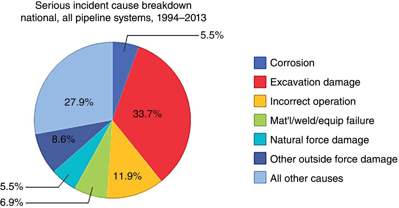
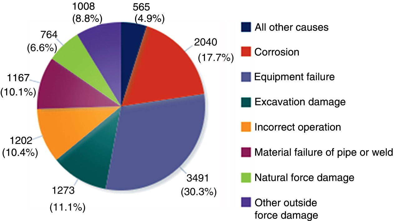
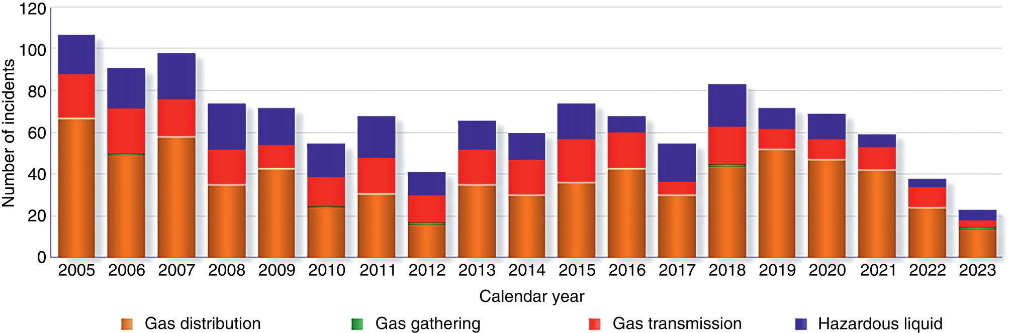
57.2 Dent Formation Process and Types of Dents
57.2.1 Dent Formation Process
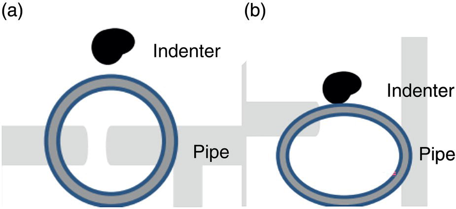
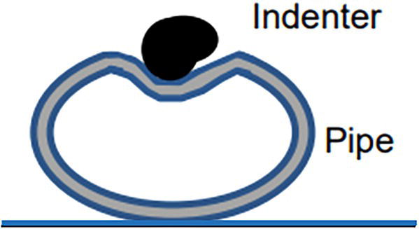
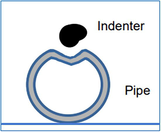
57.2.2 Common Dent Types
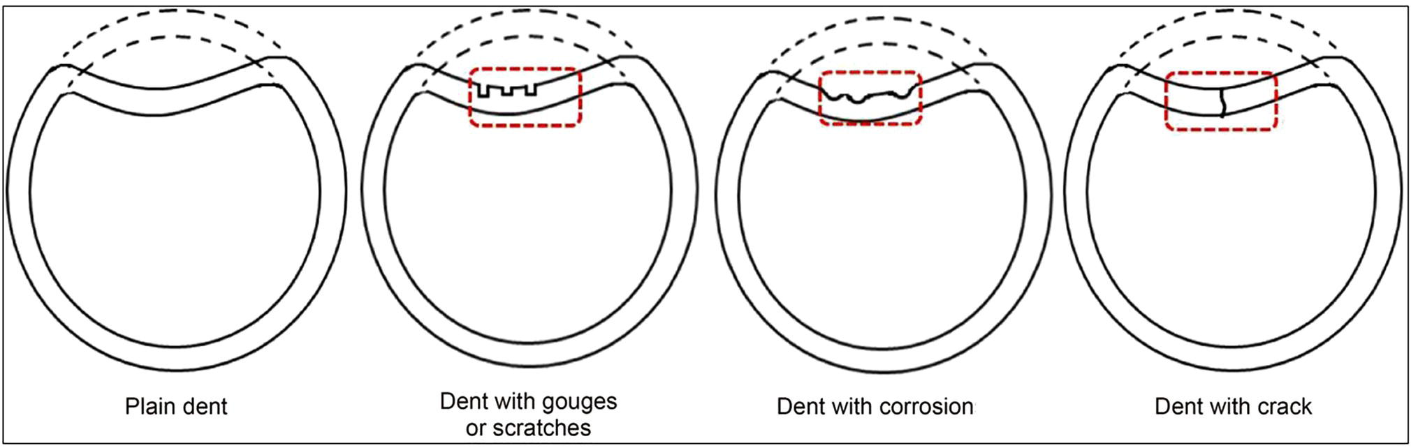
57.2.3 Coincident Features
57.3 In-Line Inspection (ILI) Technologies for Mechanical Damage Characterization [10, 11]
57.3.1 Geometry (Caliper) Sensing Technologies
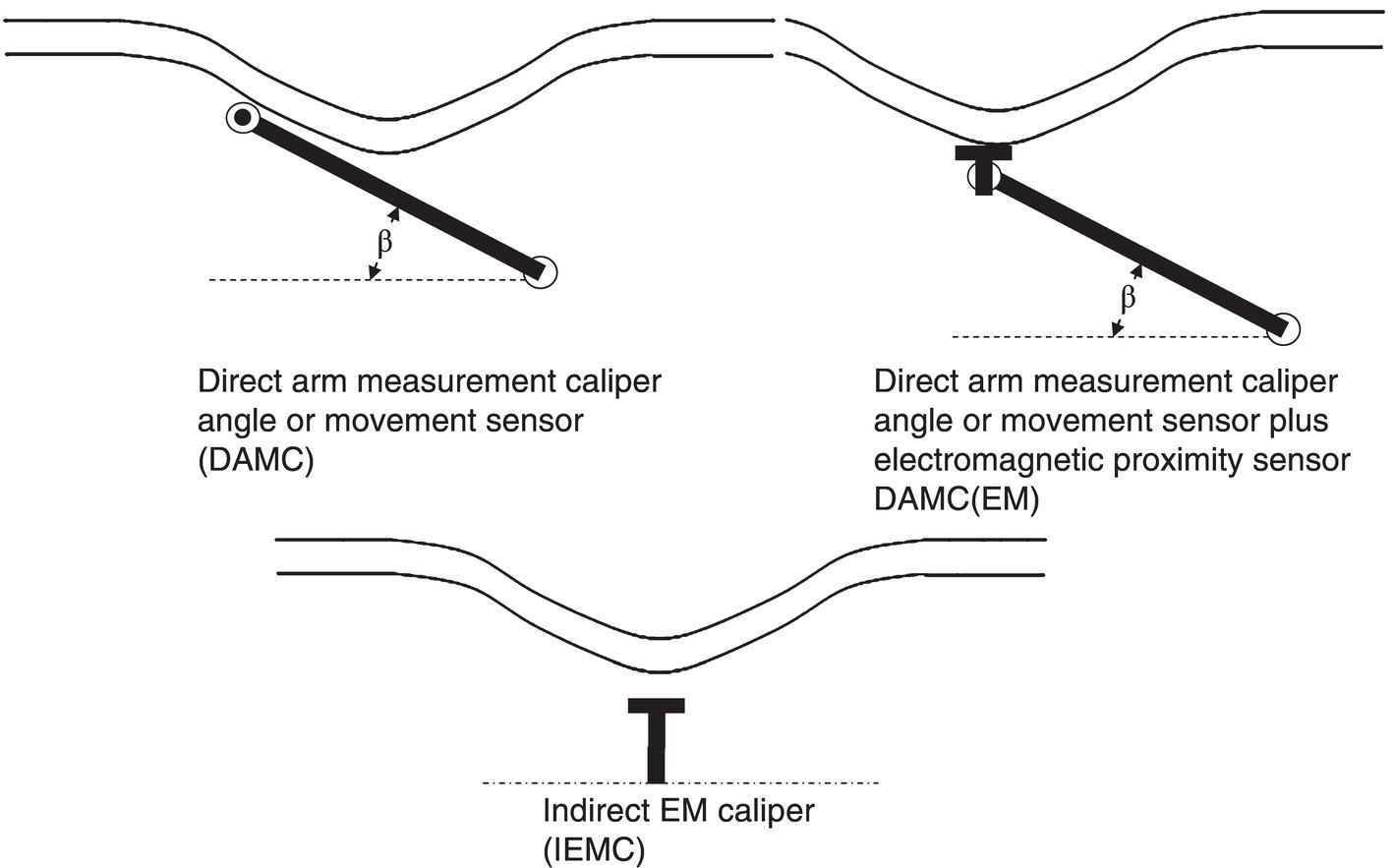
57.3.2 Coincident Damage Sensing (Dent with Metal Loss) Technologies
57.3.3 Capabilities and Performance of the In-Line-Inspection Technologies for Detection, Discrimination, and Sizing of Mechanical Damage
Generic Technology Key
Deformation Sensing Technology
Coincident Sensing Technology
Inspection Process
Caliper + MFL
Direct arm measurement caliper (DAMC)
MFL (axial magnetic field)
Two separate runs
Caliper + MFL (Circ magnet)
Direct arm measurement caliper (DAMC)
MFL (circumferential magnetic field)
Two separate runs
Caliper + MFL combo
Direct arm measurement caliper DAMC)
MFL (axial magnetic field)
One single tool, run once
Caliper (EM) + MFL
Direct arm measurement caliper (DAMC [EM]) with electromagnetic sensor
MFL (axial magnetic field)
Two separate runs
Caliper (EM) + MFL combo
Direct arm measurement caliper (DAMC[EM]) with electromagnetic sensor
MFL (axial magnetic field)
One single tool, run once
MFL (3 axes)
Tri-axial MFL Hall-3, ID/OD EM
Tri-axial MFL Hall-3, ID/OD EM
One single tool, run once
Generic Technology Type
Dent
Metal Loss
Detection
Depth
Length
Width
Detection
Depth
Length
Width
Gouge/Corrosion Discrimination
Geometry sensing technologies
Y
Y
Y
Y
Y
N
N
N
N
Caliper + MFL
Y
Y
Y
Y
Y
Y
Y
Y
N or limited
MFL (tri- axial)
Y
Y
Y
Y
Y
Y
Y
Y
Limited
57.3.3.1 Performance Measures
57.3.3.2 Dent: POD, POI, POFC, and Sizing Performance
56.6.1 Dent Sizing Performance: Vendors’ Data
Technology Type
Tolerance for Certainty = 0.8 at 95% Confidence Level
Sample Size for Validation
Limits of Detection (%OD)
Binomial Distribution Analysis (%)
Clopper-Pearson Certainty Interval Method (%)
DAMC (EM)
130a
0.5
±1.10
±1.22
DAMC (EM)
20b
0.5
±0.74
±0.74
DAMC (EM)
15c
0.5
±0.51
±0.78
MFL (3-axis)
273d
2.0
±0.78
±0.80
56.6.2 Dent Sizing Performance: Operators’ Data
 is expressed in %.
Technologies for Dents
Data Source
# of Dent Features Evaluated
Mid-range Size Caliper Specifications
Validation %D
LOD, %D
Depth Tolerance
Binomial Distribution Method
C-P Confidence Interval Method
1
DAMC(EM)
Phase I
28
0.5
±1.00
±1.60
±1.60
2
Caliper (EM) + MFL combo
Phase I
58
0.5
±1.00
±4.48
±4.65
3
Caliper + MFL combo
Phase I
17
1.0
±0.50
±1.63
1.63
4
Caliper + MFL combo
Phase II
All
135
Dents
1.00
±0.50
±1.07
±1.08
Top side
25
Dents
1.00
±0.50
±1.00
±1.20
Bottom side
110
Dents, uncorrected
2.00
±0.50
±1.10
±1.10
Bottom side
110
Dents, correcteda
2.00
±0.50
±1.32
±1.32
5
MFL (3 axis)
Phase II
All
26
Dents
0.50
±1.00
±2.40
±2.88
Top side
6
Insufficient for analysis
0.50
±1.00
NA
NA
Bottom side
20
Uncorrected
0.50
±1.00
±2.88
±3.00
Bottom side
20
Correcteda
0.50
±1.00
±0.95
±1.00
6
Caliper + MFL
Phase II
All
95
Dents
0.60
±0.80
±5.30
±5.34
Top side
1
Insufficient for analysis
0.60
±0.80
NA
NA
Bottom side
94
Uncorrected
0.60
±0.80
±5.34
±5.34
Bottom side
94
Correcteda
0.60
±0.8
±1.51
±1.52
Technologies for Dents
Data Source
# of Dent Features Evaluated
Validation of Length and Width Tolerance, inch, at 80% Certainty and 95% confidence Level
Binomial Distribution Method
Clopper-Pearson Confidence Interval Method
Length Assessment
Caliper + MFL
Phase II
28
±17.00″
±17.00″
MFL (3 axis)
Phase II
12a
±14.70″
NAa
Width Assessment
Caliper + MFL
Phase II
23
±15.00″
±21.00″
MFL (3 axis)
Phase II
12a
±20.00″
NAa
56.7 Sizing Accuracy: Pull Test Data
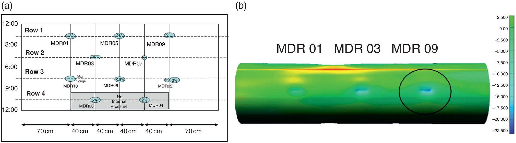
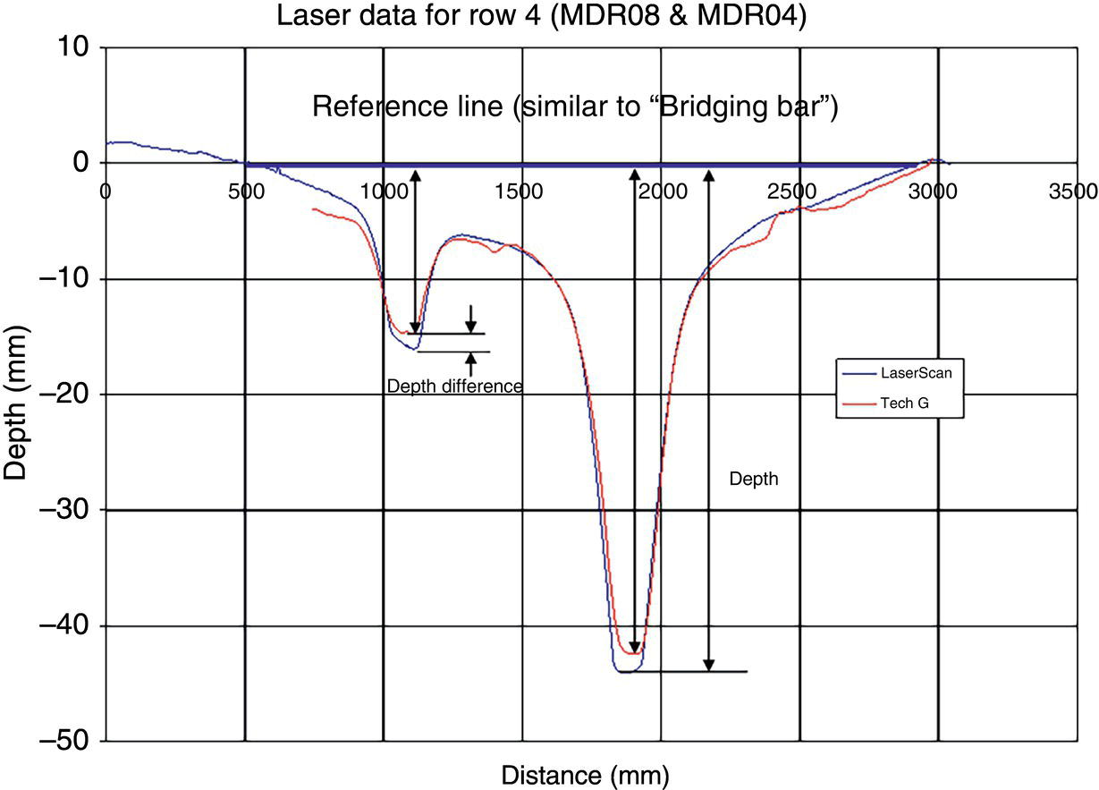
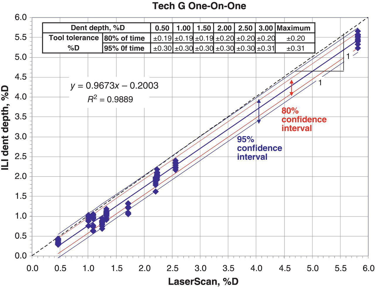
56.7.1 Sizing Accuracy: Length and Depth
57.3.3.3 Dents with Metal Loss: POD, POI, POFC, and Sizing Performance
56.7.3 Sizing Accuracy for Coincident Metal Loss
Technologies for Dents and Dents with Metal Loss
Project Phase Data Source
Total Investigations
ILI Reported DML (Exc. Based on ILI Call)
Correct Calls (Including Type of DML)
True Calls (Not Including Type of DML)
Number of Missed DML
Number of False Calls
Proportion (%)
n
x
POD
POD @ 95% Confidence Level
Binomial p, @ 95% Conf for given x, n (%)
Confidence Interval (%)
Lower
Upper
1
Caliper (EM) + MFL combo
Phase I (vendor)
138
82
27
27
18
55
60
45
27
49.0
46.7
72.3
2
Caliper (EM) + MFL combo
Phase I (vendor)
34
26
25
25
0
1
100
25
25
89.0
88.7
100.0
3
Caliper + MFL combo
Phase I (vendor)
61
58
52
49
3
6
95
55
52
89.0
86.5
98.5
4
Caliper (EM) + MFL
Phase I (vendor)
26
23
20
16
3
3
87
23
20
75.0
69.6
96.3
5
Caliper + MFL
Phase I (operator)
27
8
6
6
3
2
67
9
6
45.0
34.5
90.2
6
Caliper + MFL
Phase I (operator)
114
37
31
30
5
6
86
36
31
76.0
73.0
94.4
7
Caliper + MFL (circ magnet)
Phase I (operator)
63
56
26
22
7
30
79
33
26
67.0
63.8
89.6
8
Caliper + MFL combo
Phase II (operator)
135
135
53
53
0
82
100
53
53
94.7
94.5
100.0
9
Caliper + MFL
Phase II (operator)
94
36
33
33
0
3
100
33
33
>91.3
91.3
100.0
All
Current ILI (MFL-based) MD technologies
Combined all (1–12)
719
466
278
262
42
188
87
320
278
83.5
83.4
89.9
Technologies for Dents and Dents with Metal Loss
Project Phase Data Source
Total Investigations
ILI Reported DML (Exc. Based on ILI Call)
Correct Calls (Including Type of DML)
True Calls (Not Including Type of DML)
Number of Missed DML
Number of False Calls
Dent with Metal Loss Performance
POI
Proportion (%)
n
x
POD @ 95% Confidence Level
Binomial p, @ 95% Conf for given x, n (%)
Confidence Interval (%)
Lower
Upper
1
Caliper (EM) + MFL combo
Phase I (vendor)
138
82
27
27
18
55
100.0
27
27
89.9
89.5
100.0
2
Caliper (EM) + MFL combo
Phase I (vendor)
34
26
25
25
0
1
100.0
25
25
89.1
88.7
100.0
3
Caliper + MFL combo
Phase I (vendor)
61
58
52
49
3
6
94.2
52
49
88.4
85.8
98.4
4
Caliper (EM) + MFL
Phase I (vendor)
26
23
20
16
3
3
80.0
20
16
66.0
59.9
92.9
5
Caliper + MFL
Phase I (operator)
27
8
6
6
3
2
100.0
6
6
65.1
60.7
100.0
6
Caliper + MFL
Phase I (operator)
114
37
31
30
5
6
96.8
31
30
90.8
85.6
99.8
7
Caliper + MFL (circ magnet)
Phase I (operator)
63
56
26
22
7
30
84.6
26
22
72.7
68.2
94.6
8
Caliper + MFL combo
Phase II (operator)
135
135
53
53
0
82
100.0
53
53
94.5
94.5
100.0
9
Caliper + MFL
Phase II (operator)
94
36
33
33
0
3
100.0
33
33
>91.3
91.3
100.0
All
Current ILI (MFL-based) MD technologies
Combined all (1–12)
719
466
278
262
42
188
94.2
278
262
91.2
91.4
96.4
Technologies for Dents and Dents with Metal Loss
Project Phase Data Source
Total Investigations
ILI Reported DML (Exc. Based on ILI Call)
Correct Calls (Including Type of DML)
True Calls (Not Including Type of DML)
Number of Missed DML
Number of False Calls
POFC
(%)
n
x
POFC @ 95% Confidence Level
Binomial p, @ 95% Conf for given x, n (%)
Confidence Interval (%)
Lower
Upper
1
Caliper (EM) + MFL combo
Phase I (vendor)
138
82
27
27
18
55
67.1
82
55
75.6
57.6
75.6
2
Caliper (EM) + MFL combo
Phase I (vendor)
34
26
25
25
0
1
3.8
26
1
17.0
0.2
17.0
3
Caliper + MFL combo
Phase I (vendor)
61
58
52
49
3
6
10.3
58
6
19.4
4.6
19.4
4
Caliper (EM) + MFL
Phase I (vendor)
26
23
20
16
3
3
13.0
23
3
30.4
3.7
30.4
5
Caliper + MFL
Phase I (operator)
27
8
6
6
3
2
25.0
8
2
60.0
4.6
60.0
6
Caliper + MFL
Phase I (operator)
114
37
31
30
5
6
16.2
37
6
29.5
7.3
29.5
7
Caliper + MFL (circ magnet)
Phase I (operator)
63
56
26
22
7
30
53.6
56
30
65.1
41.8
65.1
8
Caliper + MFL Combo
Phase II (operator)
135
135
53
53
0
82
60.7
135
82
67.8
53.3
67.8
9
Caliper + MFL
Phase II (operator)
94
36
33
33
0
3
8.3
36
3
2.4
2.3
20.2
All
Current ILI (MFL based) MD technologies
Combined all (1–12)
719
466
278
262
42
188
40.3
466
188
29.5
36.6
44.2
Technologies for Dents with ML
Data Source
# of Dent Features Evaluated
Validation at 80% Certainty and 95% confidence Level, %wt
Binomial Distribution Method
Clopper-Pearson Confidence Interval Method
DAMC (EM), DAMC+MFL, DAMC(EM) + MFL combo, DAMC_MFL(circ),
Phase I and Phase II
Phase I 56, and Phase II 3
±12.0
±13.0
57.3.3.4 Closing Remarks
57.4 Technologies for In-Ditch Mechanical Damage Characterization
57.4.1 In-Ditch LaserScan Technology
57.4.1.1 Hardware: 3D LaserScanner
Technical Specifications
Model 1
Model 2
Weight
1.25 Kg (2.75 lb)
980 g (2.1 lb)
Dimensions
172 × 260 × 216 mm (6.75 × 10.2 × 8.5 in)
160 × 260 × 210 mm (6.25 × 10.2 × 8.2 in)
Measurements
25,000 measures/s
18,000 measures/s
Laser class
II (Eye-Safe)
II (Eye-Safe)
Resolution in Z axis
0.05 mm (0.002 in)
0.1 mm (0.004 in)
Accuracy
Up to 40 μm (0.0016 in)
Up to 50 μm (0.002 in)
ISO
21 μm + 100 μm/m
20 μm + 200 μm/m
Depth of field
30 cm (12 in)
30 cm (12 in) 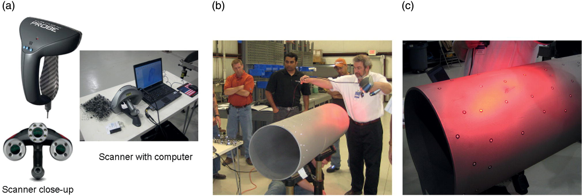
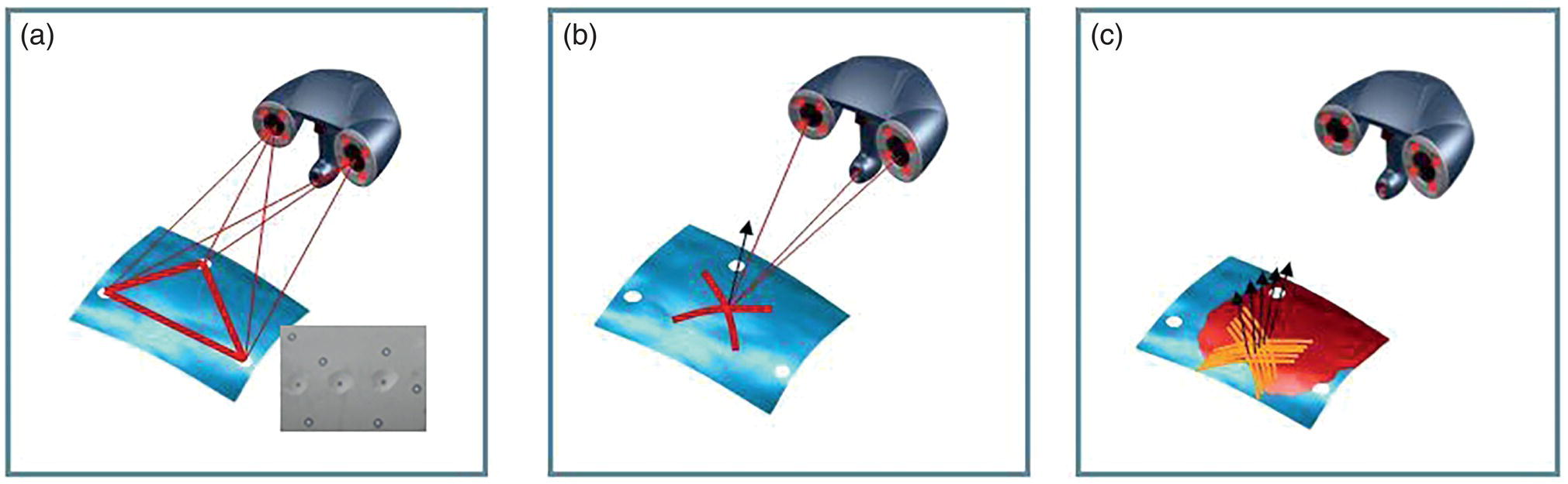
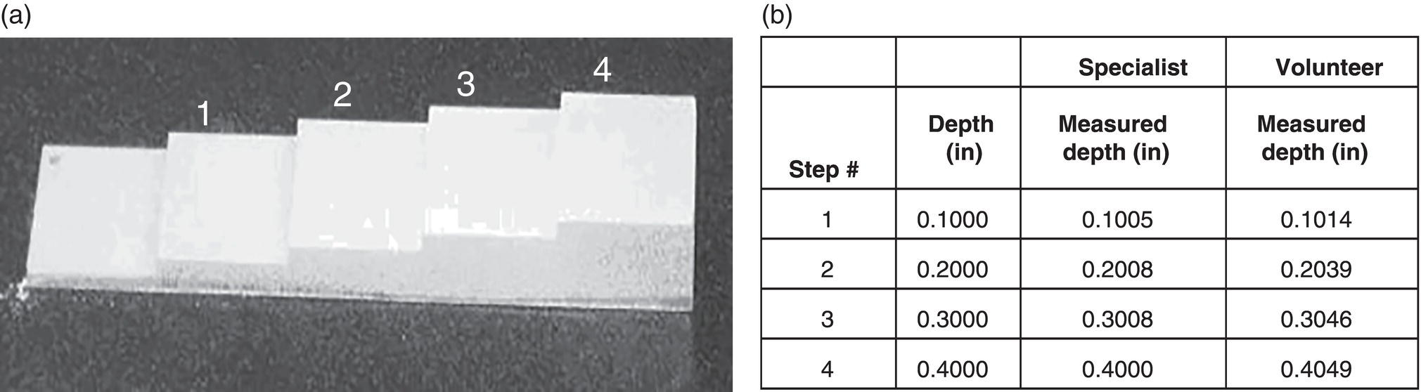
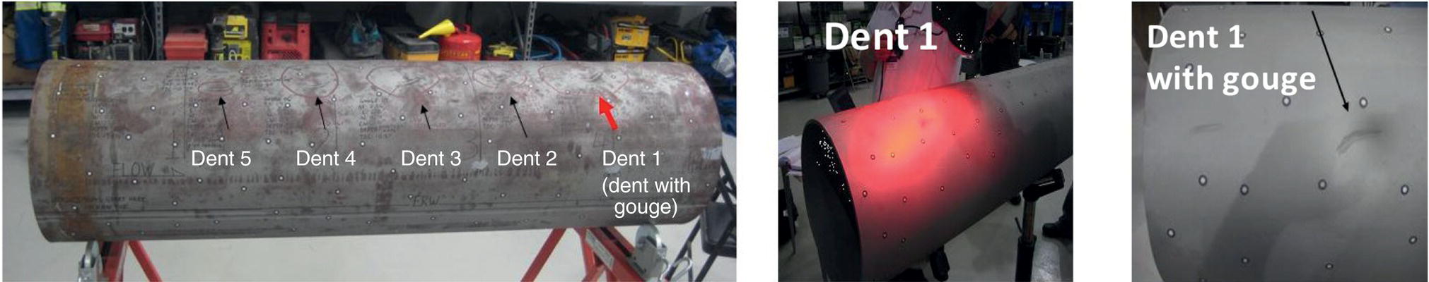
57.4.1.2 Data Processing
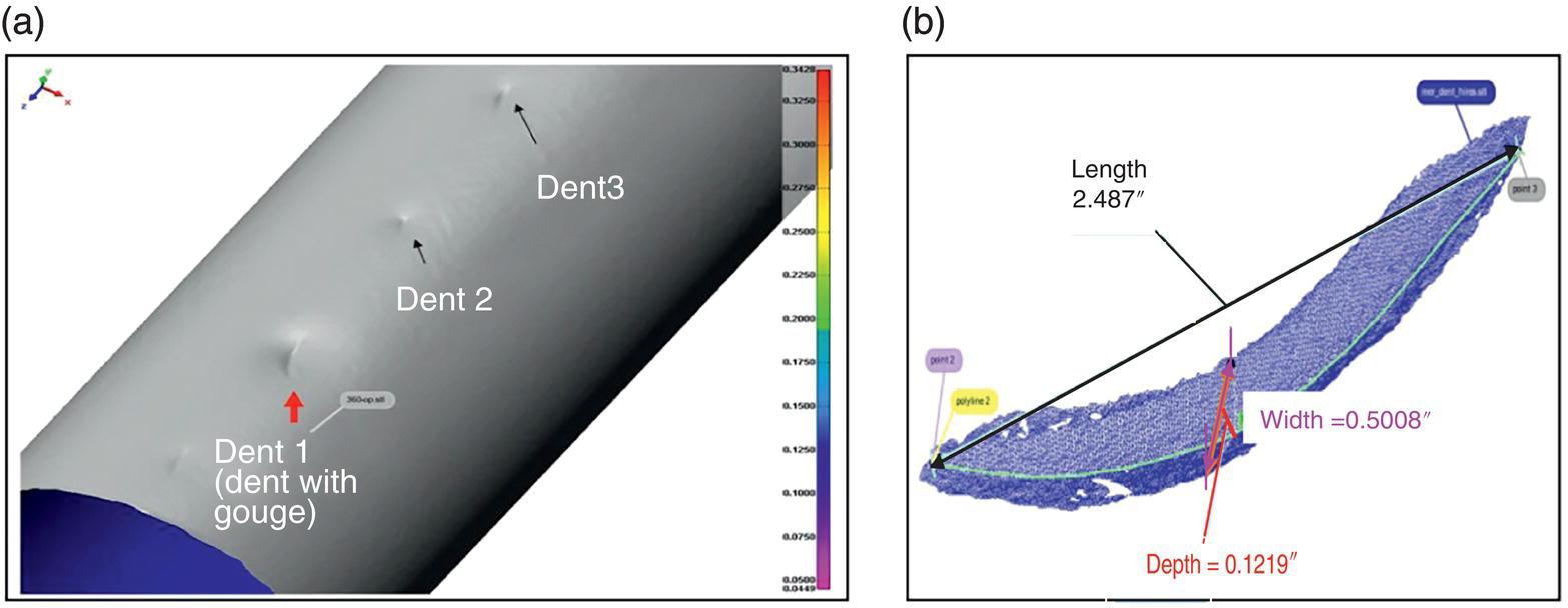
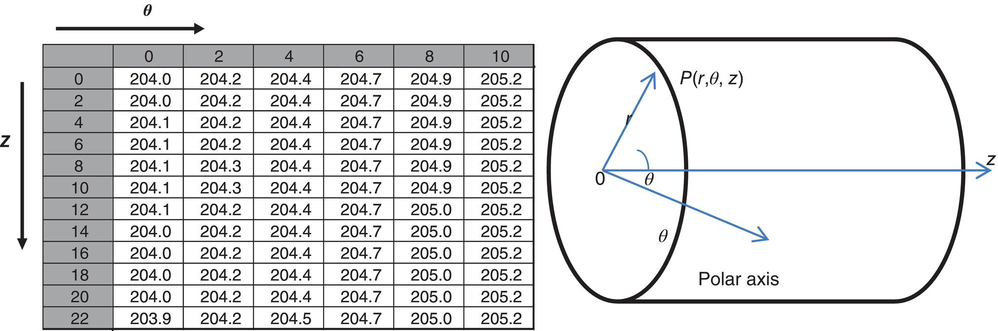
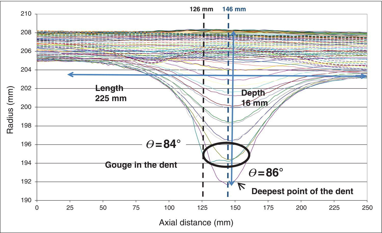
57.4.2 Application of the Improved In-Ditch Measurement Technology
57.4.2.1 Calibration of Depth-Based ILI Technologies for Mechanical Damage Evaluation [25]
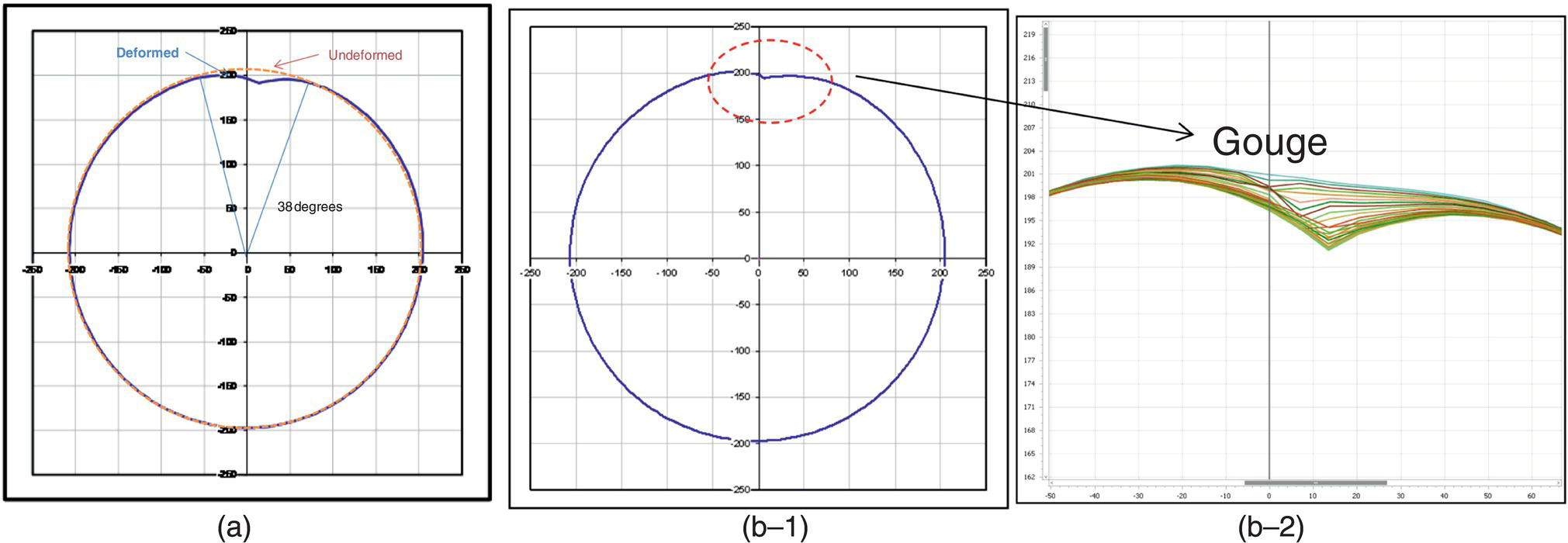
57.4.2.2 Better Evaluation of the Depth-Based Tool Performance for ILI Runs

57.4.2.3 Better Evaluation of Strain-Based Tool Performance for ILI Runs
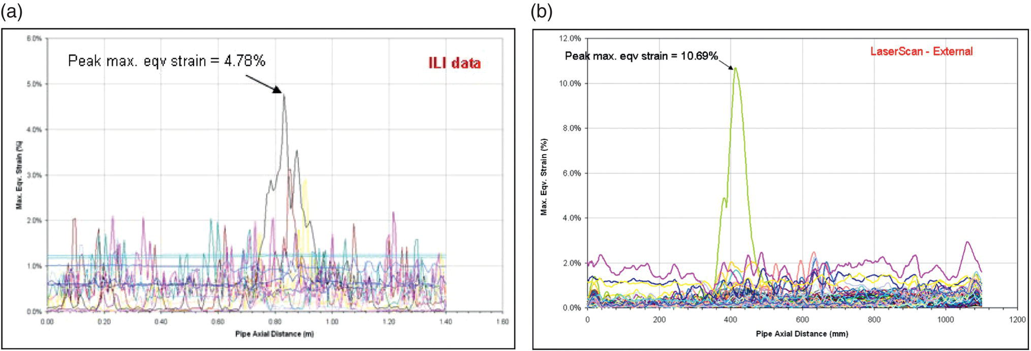

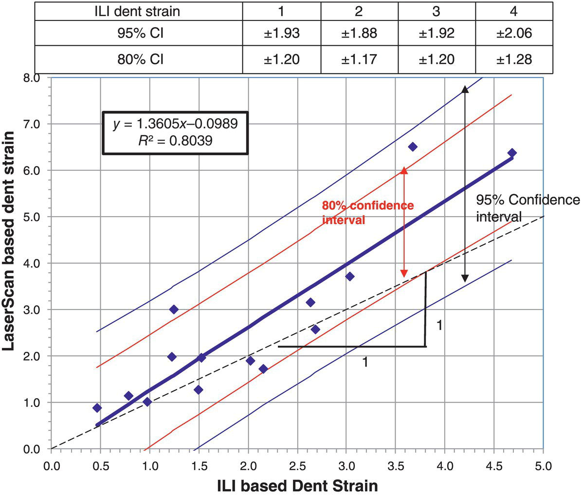
57.5 Assessment of Severity of Mechanical Damage
57.5.1 Regulatory and Industry Standard Guidance
57.5.2 Depth-Based Dent Severity Assessment
Anomaly
49 CFR 192 Condition
49 CFR 195 Condition
A dent that has any indication of metal loss, crack, or a stress riser
Immediate
Upper 2/3 of the pipe—immediate
Lower 1/3 of the pipe—60-day
A dent with depth greater than 6% of the nominal pipe diameter
Upper 2/3 of the pipe—1 year
Upper 2/3 of the pipe—immediate
Upper 2/3 of the pipe—monitoreda
Lower 1/3 of the pipe—180-day
Lower 1/3 of the pipe—monitoreda
A dent with a depth greater that 3% of the nominal pipe diameter on the upper 1/3 of the pipe
Not defined
60-day
A dent with a depth greater that 2% of the nominal pipe diameter on the upper 2/3 of the pipe
Not defined
180-day
A dent with depth greater than 2% of the nominal pipe diameter that affects pipe curvature at girth weld or at a longitudinal weld.
1-year Monitoredb
180-day
Feature
Failure Mode
Safe Limit
Mitigation
Plain, unrestrained dents (anywhere on OD)
None
6% OD: deeper up to 6% strain in pipe body. 4% strain in welds
Repair coating if excavated: monitor for corrosion if not excavated
Rock dents
Corrosion, SCC
External mechanical damage, gouges, scrapes, cracks, or SCC in dents
Rupture
None
Cut out
Low cycle fatigue
Sleeve
Grind out
Internal (pig passage) mechanical damage
None
None
None
Dents affecting ductile girth welds or seam welds
Fatigue
2% OD: deeper per analysis, subject to 4% max strain limit
Cut out
Dents on acetylene welds and brittle seams
Brittle fracture
None
Dents with metal-loss corrosion
Rupture
6% OD and metal loss per corrosion criterion
Sleeve
Dents with grind repair
Rupture
4% OD and metal loss per grind criterion
Published Guidance
Top of Line Dents (8–4 o’clock)
Bottom of line Dents (4–8 o’clock)
Plain Dent
Dents with Cracks/Gouges
Dents at Welds
Dents with Corrosion
Plain Dent
Dents with Cracks/Gouges
Dents at Welds
Dents with Corrosion
CSA Z662-03 (2005)
Up to 6% OD
Not allowed
Up to 2% for >NPS 12″ or up to 6 mm for <NPS 12″
As per ASME B31.G up to max depth of 40wt%
As for top of line dents
AS2885.3 (2001)
Up to 6% OD
Not allowed
Not allowed
Detailed assessment allowed
As for top of line dents
ASME B31.8 a(2003)
Up to 6% OD or unlimited if strain <6%
Not allowed
Up to 2% OD or unlimited if strain <4% for ductile wields (no safe limit for brittle welds)
As per ASME B31.G limits
As for top of line dents
ASME B31.4 b(2004)
Up to 6% OD
Not allowed
Not allowed
External corrosion<87.5% RWT required for design i.e. <12.5 wt. Internal corrosion as per ASME B31.G
As for top of line dents
API 1160 b(2001)
Up to 2% OD for 12a NPS (6.35MM <12″ NPS)
Not allowed
Not allowed
Not allowed
Up to 6% OD
Not allowed
Investigate/mitigate within 6 months
Investigate/mitigate within 6 months
PDAM (2003)
Up to 7% OD (unconstrained) Up to 10% OD(constrained)
Method Provided
Not allowed
Not AJ lowed
Up to 6% OD (unconstrained)
Method provided
Not allowed
Not allowed
DOT Liquid Rule (Part 195) b(2000)
1. Up to 6% OD (immediate condition) 2. Up to 3% OD for NPS? 12a or >6.35MM for NPS <12″ (60 day condition) 3. Up to 2% OD (180 day condition)
Not allowed (immediate condition)
Up to 2% OD (180 day condition)
Not allowed
Up to 6% OD
Not allowed (60 day condition)
Up to 2% OD (if >180 day condition)
Not allowed (60 day condition)
DOT Gas Rule (Part 192) a(2001)
1. Up to 6% OD for 12″ NPS or 12.7 mm for <12″ NPS (1 year condition) 2. Monitor dents >6% OD with acceptable strain levels
Not allowed (immediate condition)
1. Up to 2% for NPS 12a or up to 6.35 mm for <NPS 12″ (1 year condition) 2. Monitor dents >2% OD with acceptable strain levels
Not allowed
Monitor dents >6% OD
Not allowed
1 Up to 2% for NPS 12a or Up to 6.35 mm for <NPS 12″ (1 year condition) 2. Monitor dents >2% OD with acceptable strain levels
Not allowed
57.5.3 Static Strain-Based Dent Severity Assessment
57.5.3.1 Static Strain Calculation Equations Recommended by ASME B31.8
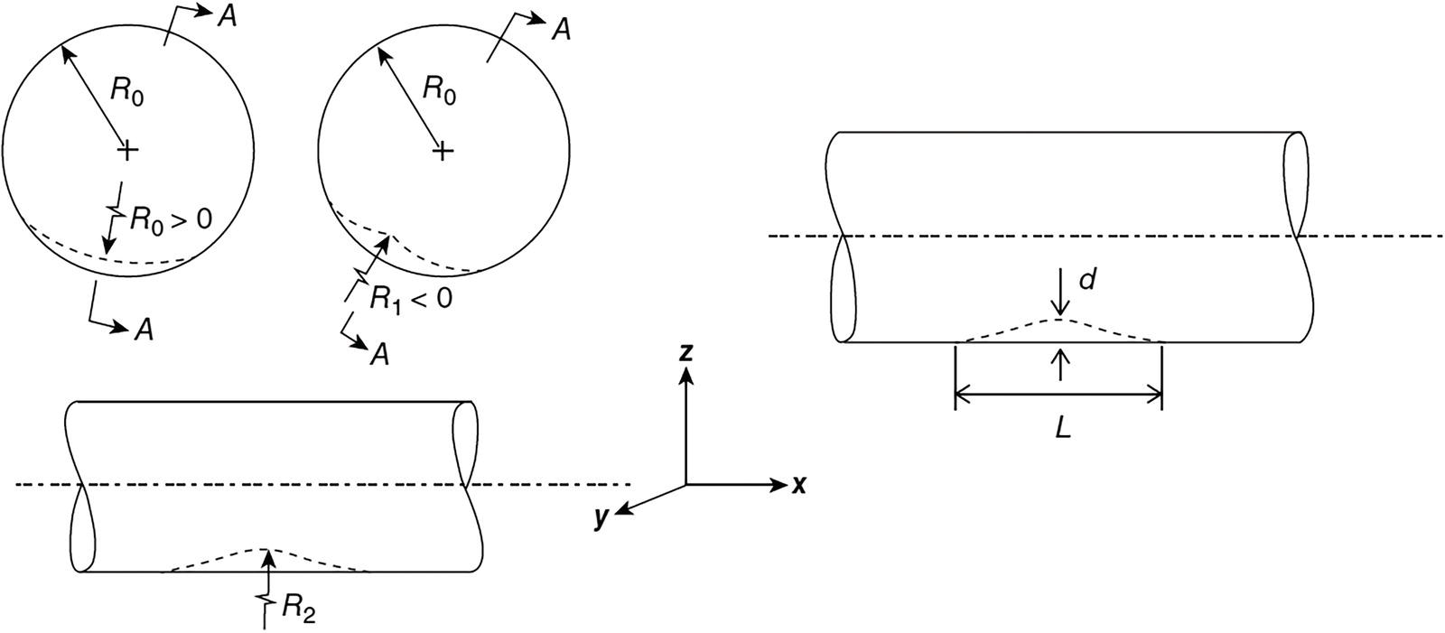
 where e1 = ε1, e2 =ε2 + ε3, e3 = 0 without having a preceded constant 2/3, or can be thought of as analogous to von Mises stress for a plane stress condition,
 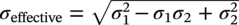 where σ3 = 0.
 [35].
[35].
57.5.3.2 Improved Static Strain Calculation Methods
Lukasiewicz Method
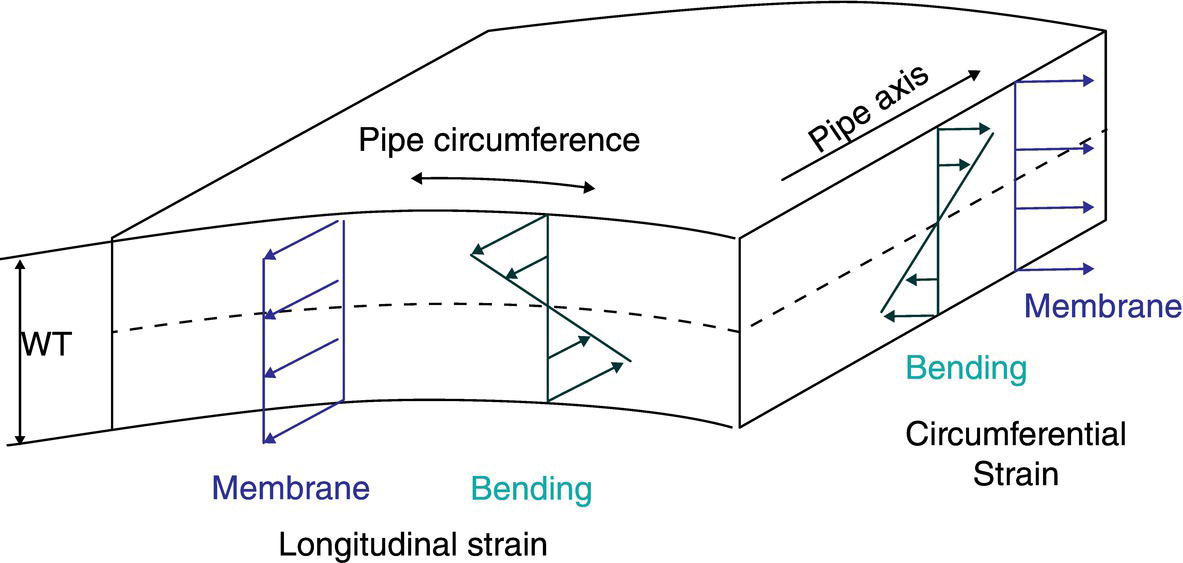
 and
and  , can then be calculated from the curvature of the radial displacement w in the axial x and circumferential y directions (see Figure 57.25).
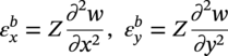
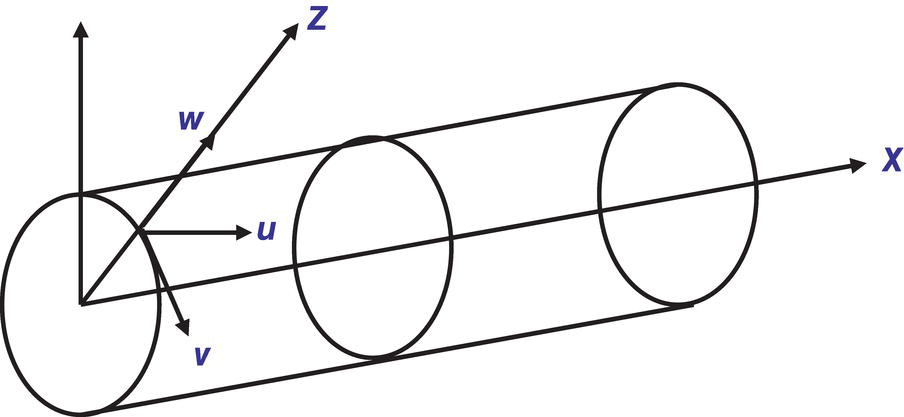
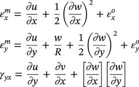
 and
and  are the membrane strains in the axial (x) direction and the circumferential (y) direction, respectively.
 and
and  are the initial strains due to the pressure in the pipe, thermal expansion, etc.
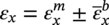
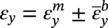
 ), and (2) a sign difference in the mid-term εxεy. These differences could result in a significant discrepancy in the calculated effective strain value. Czyz et al. [34] demonstrated that the difference in effective strain can be more than 50% with the assumption that
  = 0. Further comparison [34] was made using the three-case data provided by Baker [17]. Again, the comparison assumes γxy = 0. The results showed that ASME B31.8 Equation (57.8) underestimates the effective strain by a factor of up to 1.8 and 2 for external and inner surfaces, respectively, which is significant.
Blade Energy Partners Simplified Mode [35, 41, 58, 59]
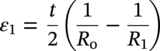 and
and 

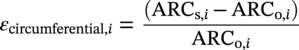
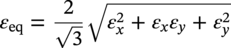
Dent Depth, %OD
Maximum Eqv. Strain
% of error = (Blade Strain-FEA Strain)/FEA Strain (%)
Blade’s Dent Analyzer Tool (%)
FEA (%)
3.0%
11.9
11.6
2.6
6.0%
22.2
25.1
−11.4
9.0%
24.6
26.5
−7.3
12.0%
29.6
29.7
−0.3
15.0%
30.1
31.3
−3.9
Re-bound
31.5
31.3
0.5
Average
−3.3
Stdev
5.3
57.5.4 A Combined Approach to Evaluate Dent with Metal Loss
57.5.4.1 Static Dent Strain-Severity-Based Criterion
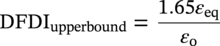
Case
εeq (%)
Upper-bound DFDI
Prediction
Excavation
Prediction-Excavation
1
10.20
0.6
Possible crack
Through wall crack
Positive-positive
2
15.00
0.8
Possible crack
Through wall crack
Positive-positive
3
16.90
0.9
Possible crack and gouge
Gouge
Positive-positive
4
13.00
0.7
Low confidence of possible crack
ID crack
Positive-positive
5
31.00
1.7
Crack with MD
MD
Positive-positive
6
17.60
1
Possible crack
ID/OD crack
Positive-positive
7
11.50
0.6
Possible crack
Through wall crack
Positive-positive
8
6.80
0.4
Not crack
No crack but 6% “ML”a caused by sitting on rock
Negative-negative
9
7.10
0.4
Not crack
No crack but 16.4% “ML”a caused by sitting on rock
Negative-negative
10
10.50
0.6
Not crack
No crack but 12% “ML”a caused by sitting on rock
Negative-negative
11
9.90
0.5
Not crack
No crack but 16% “ML”a caused by sitting on rock
Negative-negative
12
5.00
0.3
Not crack
No crack but 36% corrosion
Negative-negative
13
9.00
0.5
Not crack
No crack but 10% “ML”a caused by sitting on rock
Negative-negative
14
7.80
0.4
Not crack
No crack but 15% corrosion
Negative-negative
15
3.60
0.2
Not crack
No crack but 37% corrosion
Negative-negative
57.5.4.2 MFL-Signal-Criterion
57.5.4.3 Illustration of the Effectiveness of the Approach: Case Study
57.5.5 Dynamic Strain-Based Dent Severity Assessment
57.5.5.1 Rate and Temperature-Dependent Damage Criteria
 is equivalent plastic strain in each increment and
  is rate-dependent failure strain, as defined in Equation (57.19):
 is plastic strain rate, and σm/σeq is stress triaxiality.
57.5.5.2 Dynamic Versus Static FEA for Dent Formation
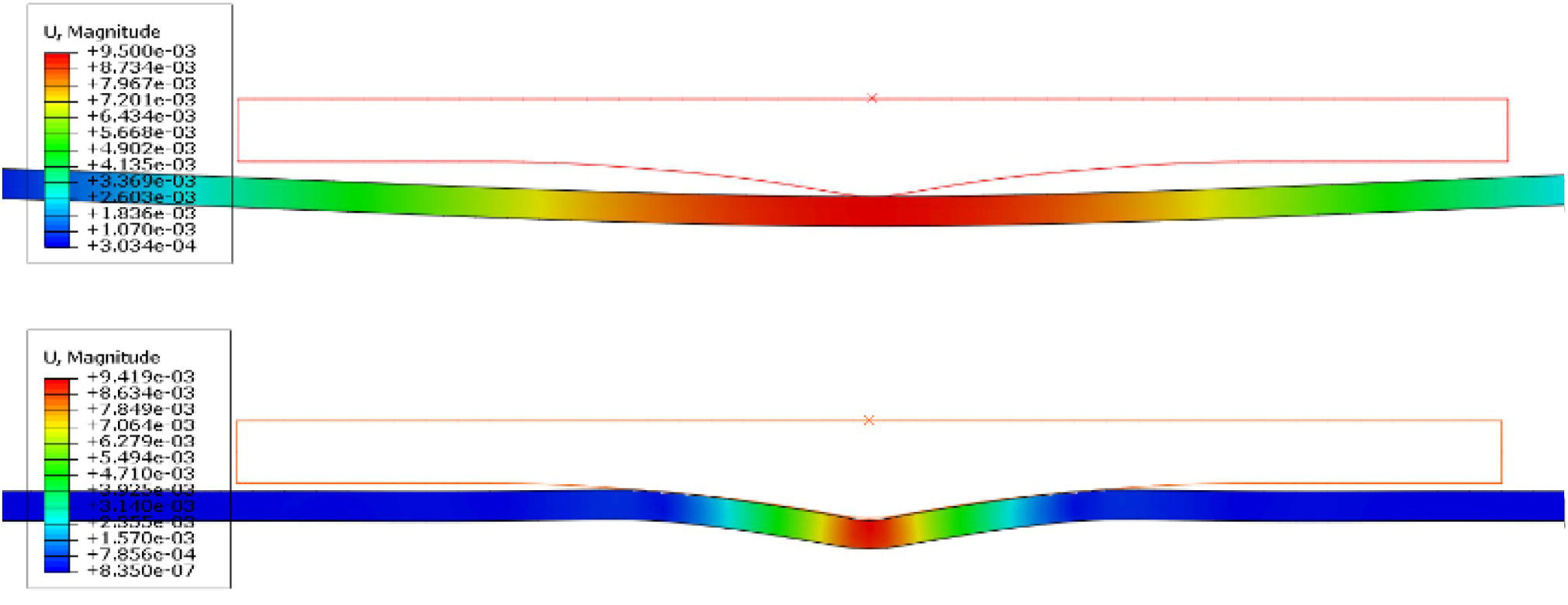
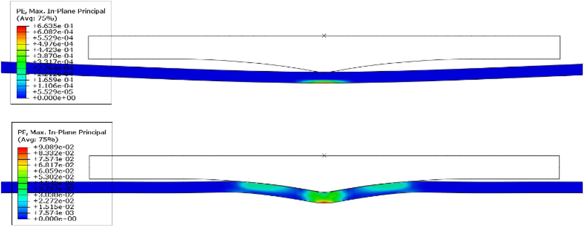
57.5.5.3 A Multi-Element Dent Assessment Approach
57.5.5.4 Closing Remarks
57.5.6 Fatigue-Based Dent Severity Assessment
57.5.6.1 Level 1 Assessment: Dent Geometry Severity Ranking Approach
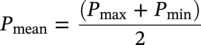
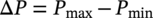

57.5.6.2 Level 2 Assessment
Level 2 Assessment—BMT/PRCI Approach
Level 2 Assessment—EPRG/API 579 Approach
57.5.6.3 Review of the Scientific Basis of the EPRG 2000 Model

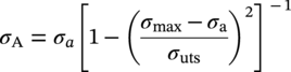
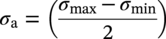
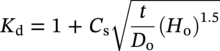
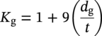
57.5.6.4 Improvement of the EPRG 2000 Equation and Validation
57.5.6.5 Execution of the Modified EPRG Model: Excel Based Software
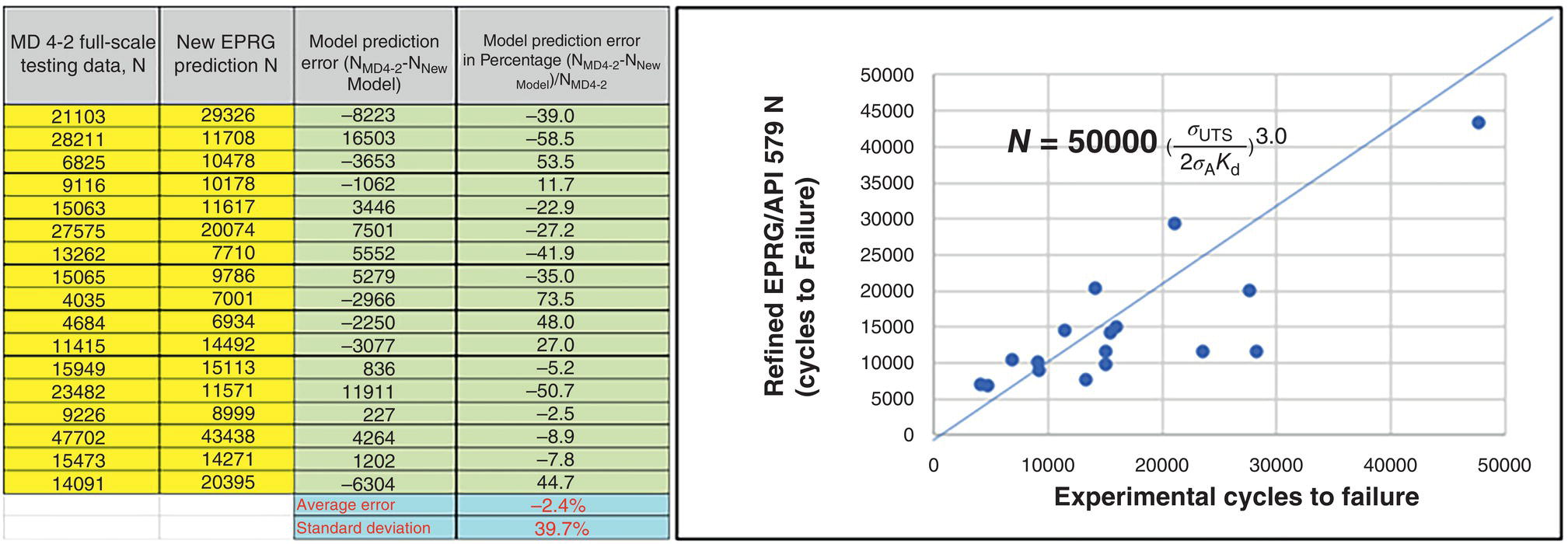
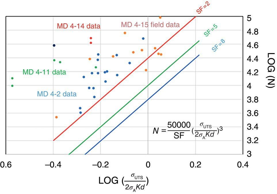
57.5.6.6 Level 3 Dent Fatigue Life Assessment
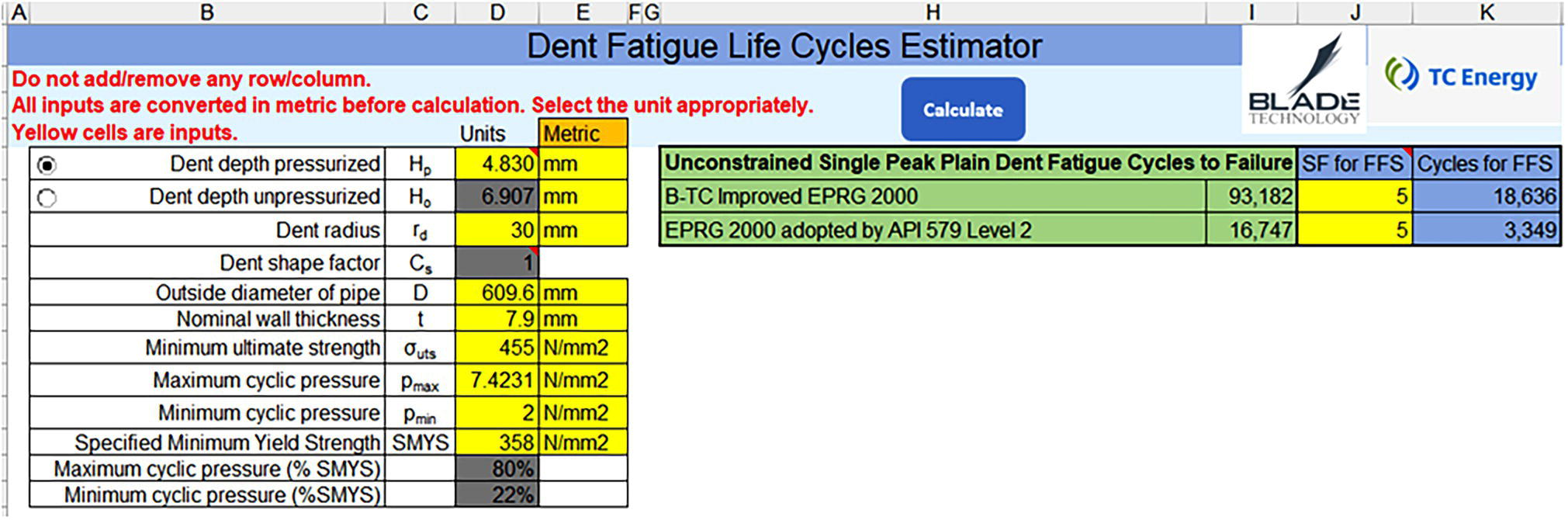
57.5.6.7 Comparison of the Improved EPRG Equation with BS 7608 Class D and FEA Model for Fatigue Life Prediction
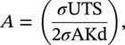 which is the opposite used by the API RP 1183 plot. In addition, the API RP 1183 plot only includes two sets of test data, i.e., M 4-2 and MD 4-11 data with two lines: model prediction and model prediction minus one standard deviation (1 st dev). Therefore, two changes are made to the modified EPRG plots for comparison, accordingly.
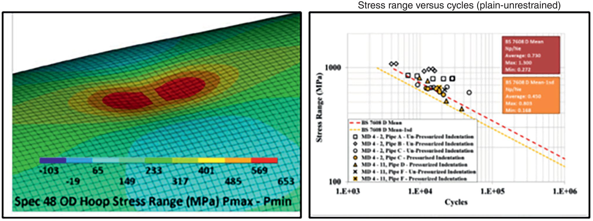
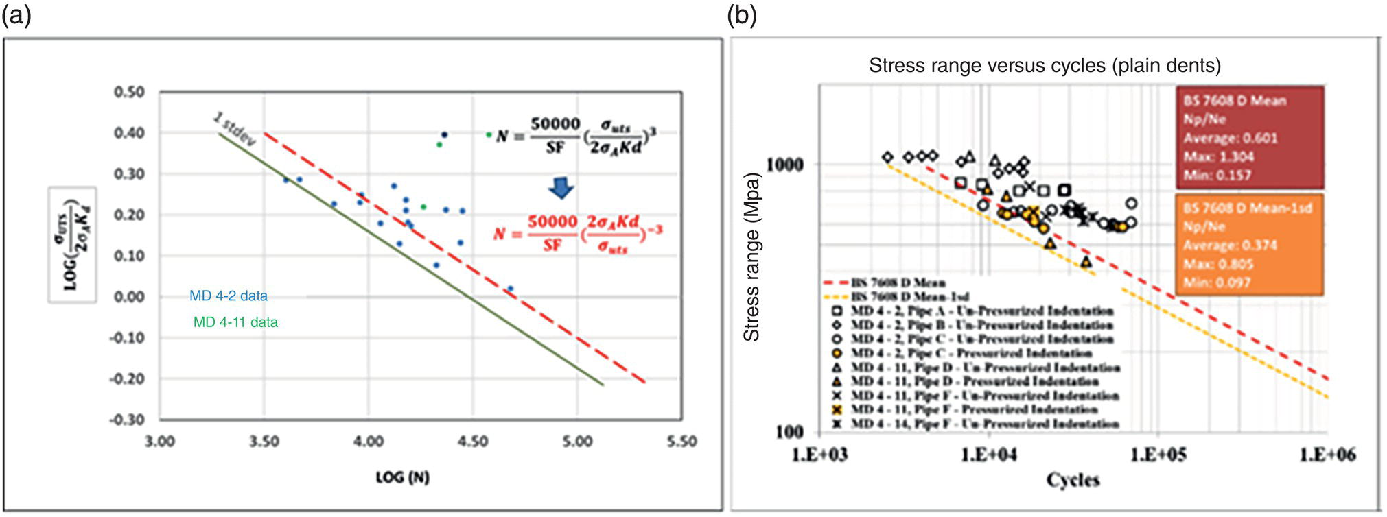
57.6 Mitigation and Repairs
57.6.1 Improved Strain-Based Dent Severity Criteria—Alternatives
57.6.1.1 Criterion Based on Ductile Failure Damage Indicator (DFDI)
 , and the material’s critical strain, εo:
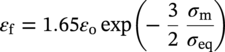
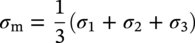
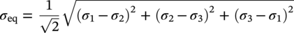
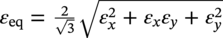 (i.e., Equation (57.12) in Section 57.5.3) and D is the ductile failure damage indicator ranging from 0 (undamaged) to 1 (cracking). By the definition, ductile failure or failure of dent (cracking) will occur when D > 1. In order to calculate the DFDI, finite element analysis should be conducted to extract three principal stresses and the equivalent plastic strain at every node on the dent deformation region. However, it is not practical to conduct FEA for all reported dents in the pipeline. Most recently, the present authors developed simplified DFDI equations [1, 2, 60, 61] which do not use FEA result and also validated against FEA prediction. Following are the simplified DFDI and SLD equations.
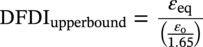
57.6.1.2 Criterion Based on Strain Limit Damage (SLD)

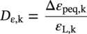
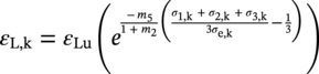
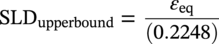
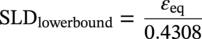
57.6.1.3 Specified Minimum Engineering Criterion
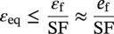
57.6.2 Repairs
57.7 Continued Challenges
References
Note
Mechanical Damage in Pipelines: A Review of the Methods and Improvements in Characterization, Evaluation and Mitigation
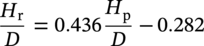
(57.2)


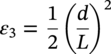
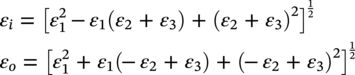
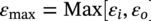
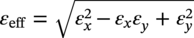
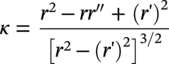
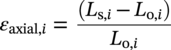
(57.11)
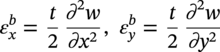
(57.13)
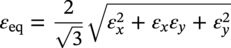
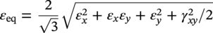
(57.16)
(57.17)
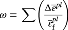
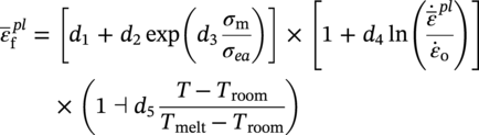

(57.21)
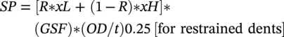


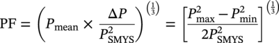

(57.27)
(57.28)
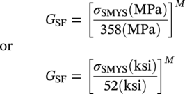
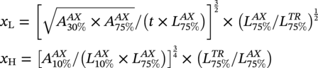
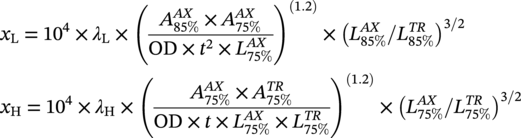
(57.32)
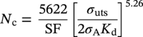
(57.34)
(57.35)
(57.36)
(57.37)
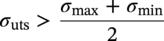
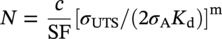

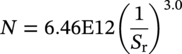
(57.42)
(57.43)
(57.44)
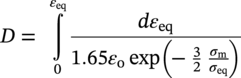
(57.46)
(57.48)
(57.49)
(57.50)
(57.51)
(57.52)
(57.53)