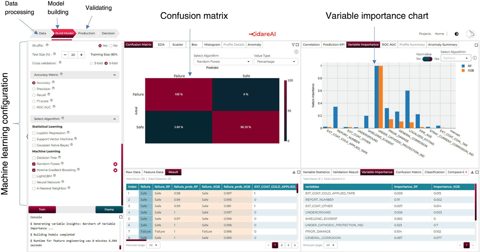
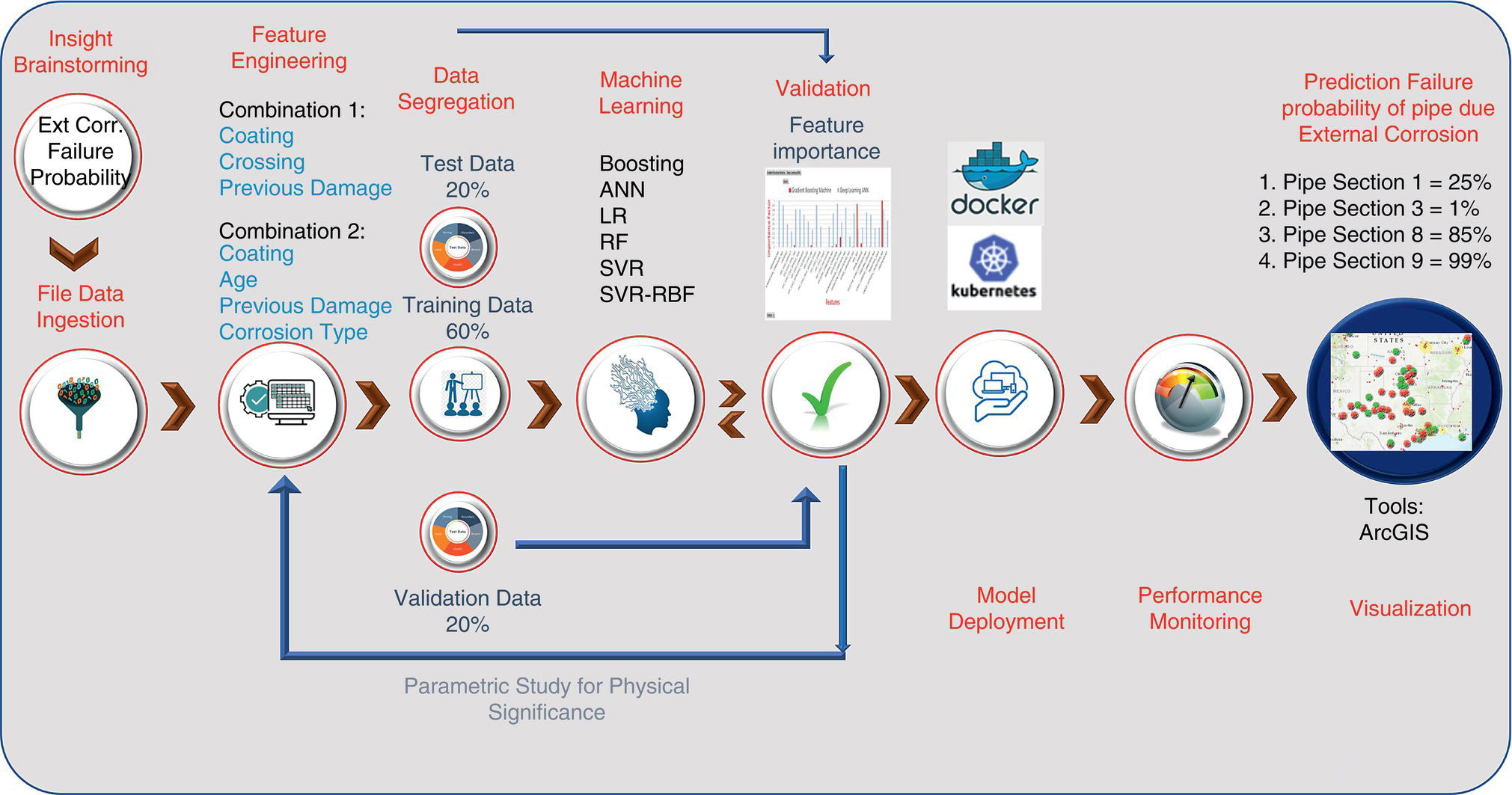
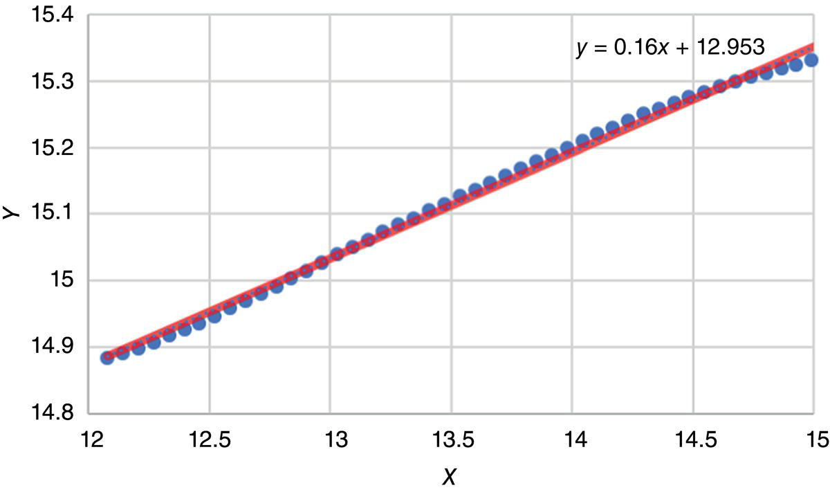
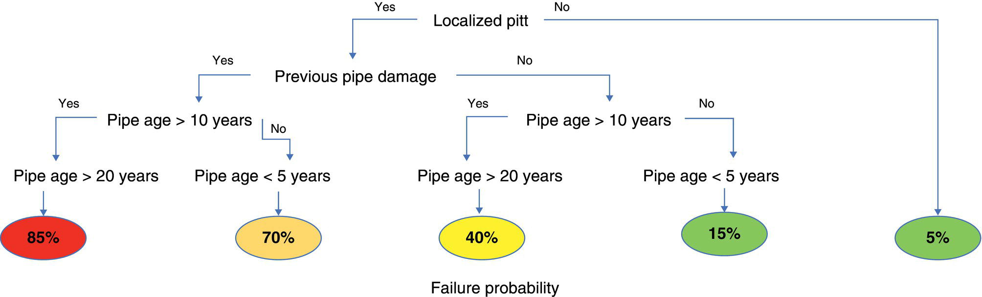
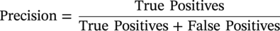
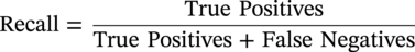
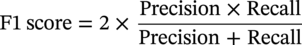
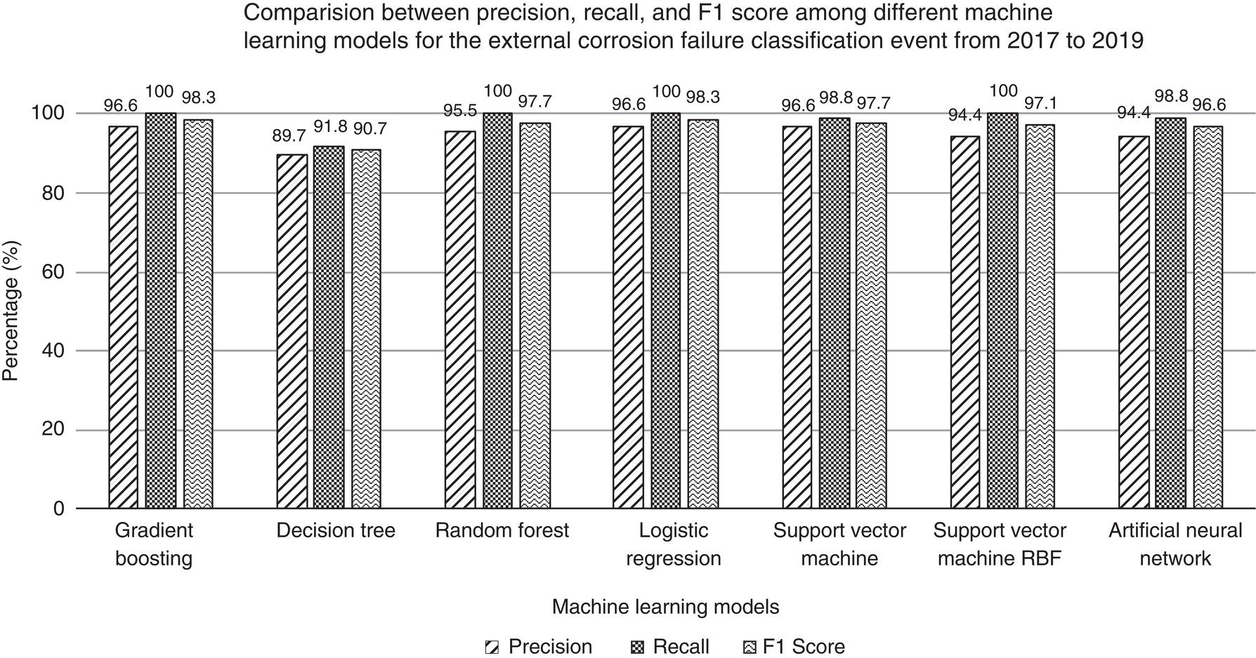
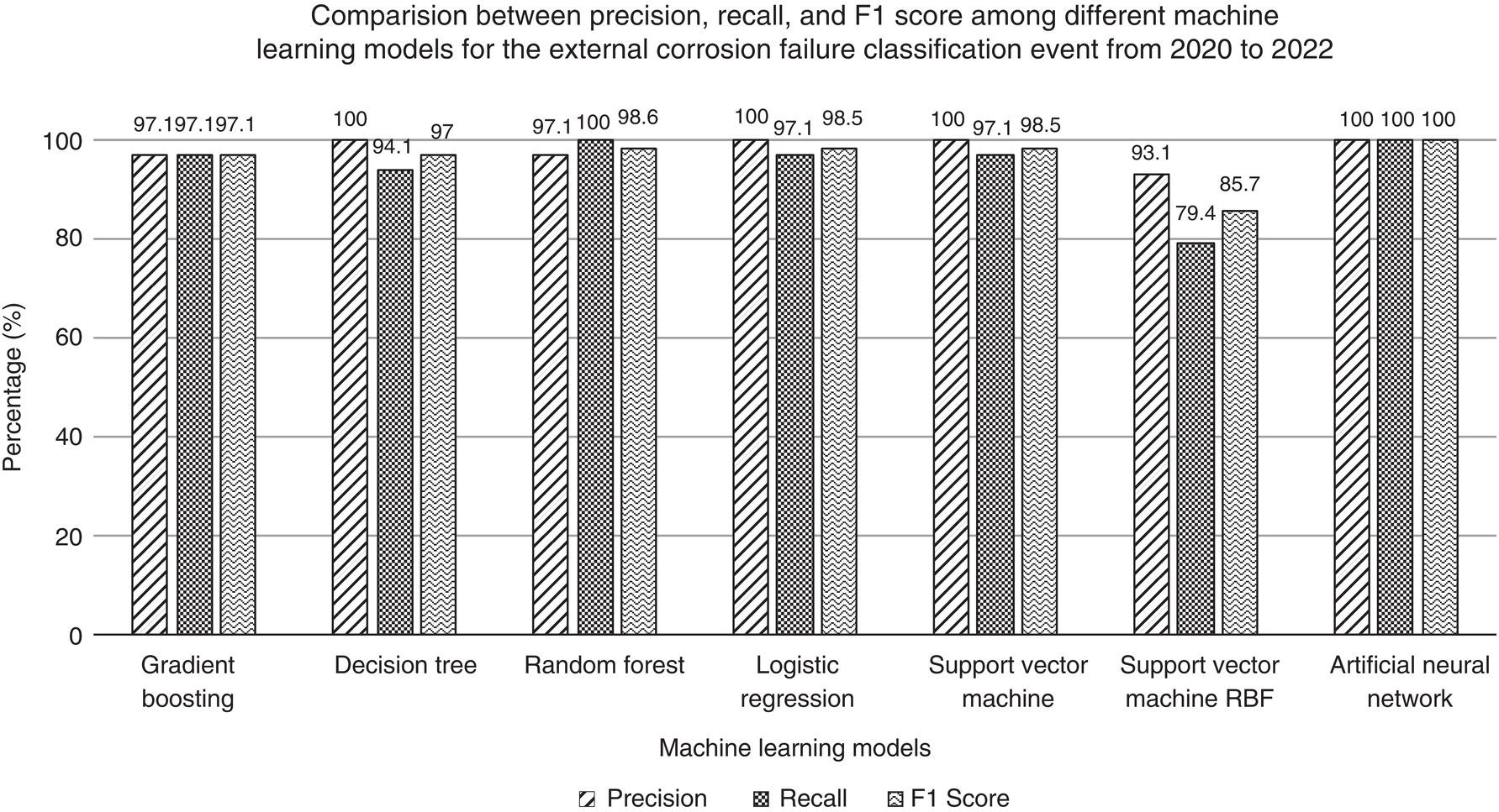
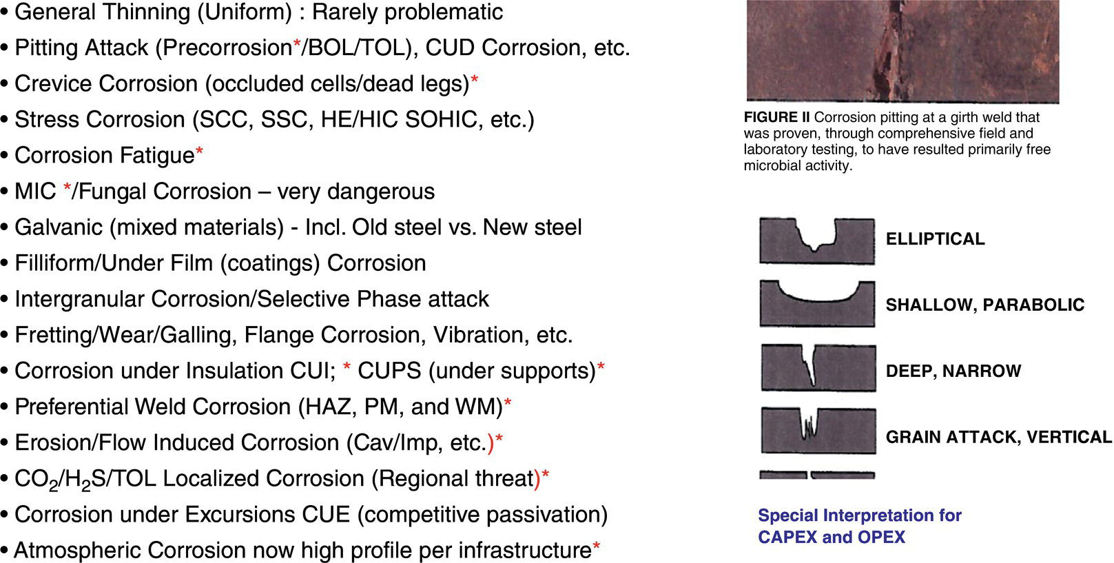
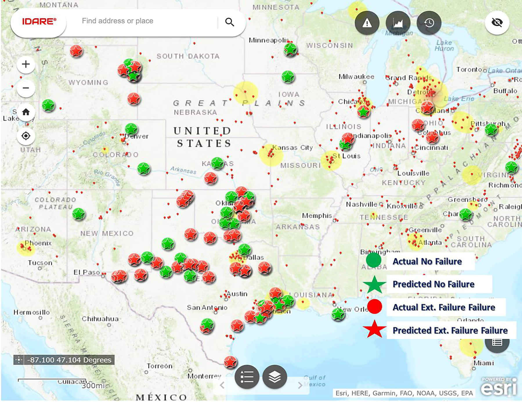
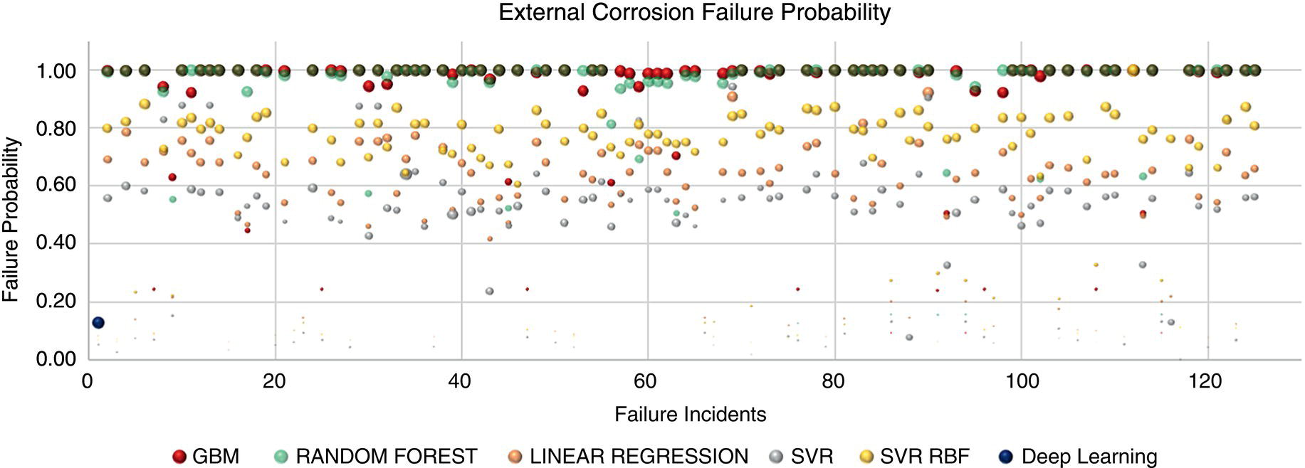
Khairul Chowdhury1 Binder Singh2 and Shahidullah Kawsar1 1IDARE LLC, Houston, TX, USA 2PragmaticaGGS, Cypress/Houston, TX, USA In the early days of corrosion engineering maturation, Fontana and Greene [1] from the Ohio State University and Rensselaer Polytechnic Institute, respectively, described the eight forms of corrosion, with many subgroupings. Expansion of knowledge and the use of new materials, welding techniques, surface treatments, new coatings, inhibitors, and exposure to more aggressive environments, etc. have led to recognition of over 18 corrosion mechanisms, each with its own characteristics and possible solution options. In addition, corrosion monitoring and inspection techniques have evolved to address difficult situations. In Table 4.1, techniques, methodologies, and adapted tools are summarized, and the risks and roles of AI-ML are annotated for each technology. After the realization that many engineering failures were in fact related to corrosion phenomena, the global drives toward improved mechanical integrity management led to the creation of corrosion management, later expanded to corrosion and integrity management (C&IM). Since, this is primarily a prevention or life cycle repair/retrofit exercise, the driving force was always the cost or return on investment (ROI); hence, the favored route of assessment is to mitigate risks without expensive testing, field trials, or data mining, a formidable challenge that has led to extracting, and “culling” data across assets and even industries to redeploy on a particular project. Most judgments are made by practical experience and fundamental understanding of the dominant corrosion mechanisms, with advanced corrosion failure risk assessment and existing computer techniques. The impact of AI-ML in this regard has thus become self-evident, with a natural evolution to machine intelligence (MI). The ability and feasibility of artificial intelligence and machine learning (AI-ML) techniques to leverage characteristic inspection data are powerful, leading to prediction of corrosion failures via mimicking practical experiences. In this chapter, the applications of computer-based analytical techniques in corrosion science are presented and discussed for the direct benefit of the rapidly growing disciplines of corrosion and integrity management [Refs. 2–5], including the best practice of full life cycle integrity management. Qualitative risks related to external and internal corrosion of pipelines were examined using six different AI and ML algorithms leveraging existing PHMSA Hazardous Liquid Accident reports. The importance of insights and governing mechanisms for corrosion-related failures were identified utilizing key AI-ML algorithms. Where feasible semiquantitative risk assessments were used to perform a “calibration check” on the findings. For the best utilization of learning algorithms like gradient boosting, deep learning, support vectors, random forest, decision trees, and logistic regression, singular corrosion mechanistic pipe failure can be predicted with 97% accuracy. In practice, the combination of “When and Where” remains a challenge that can be better appreciated as the AIML feedback loop self-improves after the first iteration. Importantly, since AI-ML has no “emotional” content, lessons learned (LL) are better identifiable and applied without negative human factors interference; nevertheless, the human touch must be “mandated” to fine-tune, sift, and explore data trends so that errors do not overturn the benefits of evidence and relevant experience. The AI-ML process is automated in a cloud-based web application format to help predict failures from raw characteristic data of accident reports along with corrosion SME verification or field validation. High accuracy and reliability of failure prediction demonstrate that the use of AI will enable decision-makers to provide speedy and more confident interpretation of corrosion risks. As AIML capabilities are developed, the need for human engagement will diminish to smaller-scale oversight. Table 4.1 Corrosion Monitoring Selection General Guide Most techniques are project specific and “in line” and also possibly utilized via bypass loop. Legend: generally Good √ Not so good × Debatable √×. a N/A Not Applicable—sometimes difficult to justify. Note 1: Probes/coupons must be placed at least 10 diameters downstream and at least 3–5 diameters upstream of any fittings/valves, discontinuities, etc. to minimize flow interference. Note 2: Most techniques can be tested in the lab and adapted in the field. Always vital to use a meaningful control. The work that is now being done worldwide will form the basis or platform for future efforts, and in that regard just as the data scientists must be well versed and qualified in the subject matter, so must the corrosion experts. Inadequacies in that regard will lead to misinterpretation and dangerous misappropriation. Such proper SME engagement will always be the check and balance against outlying, over-fitting, and under-fitting data; and the value of continuous learning may be the biggest single advantage. The literature on corrosion science, corrosion engineering, corrosion testing, and integrity management is vast, though most of the pertinent information and data remains in the “libraries” of private companies due to competitive advantage and IP retention. Some of this information is disseminated by various joint-industry projects (JIPs) and the “not-for-profit” societies such as AMPP, IMECHE, IMAREST, ASME, SPE, DNV, LR, ABS, and BV. Most of that information is available in the public domain through relevant topical papers and web pages and a selection is presented in the references and bibliography of this chapter [1–35]. However, readers should be aware that web pages, while valuable, are prone to be changed. Likewise, the history and evolution of AI-ML is a massive collection of papers and articles, official and unofficial. These are best listed as contact points to eliminate the possibilities of nonproductive direction. There are also many researchers who have been using machine learning algorithms to advance corrosion knowledge. Image recognition machine learning models have been used to detect corrosion in certain cases. Luca et al. [29] used computer vision technique to detect corrosion from images of structures mostly applicable for bridge inspection. Nash et al [11] investigated the impact of dataset size on deep learning for automatic detection of corrosion of steel assets. Ortiz et al. [12] proposed a defect detection approach comprising a microaerial vehicle. In many studies, machine learning has been used to explore mechanisms that affect corrosion of steel pipelines, although the use of AI in corrosion started as early as the 1980s. Hernandez et al. [13] evaluated artificial neural networks (ANNs) for predicting the corrosion inhibition offered by crude oils as a function of several of their properties. Vancoille et al. [14] investigated the assessment of corrosion and related risk behavior in oil refinery operation based on practical experience and a basic understanding of the prevailing corrosion mechanisms. Lajevardia et al. [16] assessed the capability of an ANN for estimating the time to failure by SCC of Type 304 stainless steel (UNS No. S30400) in an aqueous chloride solution. An ANN was used to predict corrosion loss of structural carbon steel in the atmospheric environment; i.e., temperature, relative humidity, air pollution by sulfur dioxide, and exposure time. Although there are uses of AI to predict corrosion-related phenomena for steel, neural networks are most commonly used. Mohd et al. [41] studied machine-learning-based classification for pipeline corrosion with Monte Carlo probabilistic analysis. Geovanni et al. [42] investigated a transfer-learning approach for corrosion prediction in pipeline infrastructure. In this study, the effectiveness of neural networks in predicting corrosion-related phenomena was also investigated and compared with other machine learning methods. Most machine learning methods require an extensive amount of data to achieve a predictive ability. In this chapter, a data science technique is presented that has the ability to predict with high accuracy using very low-resolution, unstructured data. The use of advanced but now recognized approaches of BAST, ALARP, and ISD can be used as guidelines to prevent and control corrosion and integrity threats before any serious damage is done to the asset, facility, equipment, component, or feature [6, 20, 22, 24]. The combined disciplines of AI-ML and corrosion are in a growth mode, and it is recognized that the development of AI-ML technologies for predicting corrosion performance will provide significant benefits across all industries. In order to provide data-driven decision making and generate actionable intelligence, an automated codeless intelligent predictive analytics computation system, known as idareAI, has been utilized. The idareAI engine is an autonomous engine configurable for solving different decision-making problems for different disciplines. Figure 4.1 shows a schematic of the codeless machine learning engine and how it works. The engine includes a complete suite for data ingestion from various data sources, data cleanup processing, and a comprehensive suite of machine learning algorithms to provide extensive insights and data visualization digital twin for visualizing insights. AI-ML is prone to influence via relatively small changes in conditions and so it is important to work with SMEs, e.g., in corrosion, structural, metallurgical, and flow assurance. Figure 4.1 Steps of machine learning followed through automated machine learning engine. In order to generate corrosion failure insights from the low-resolution accident reports, a comprehensive methodology was followed to incorporate subject matter expertise, physical mechanism, and data governance. At least 50 parametric studies were performed to understand the importance of characteristics of a pipe section over external or internal corrosion failure. The solution methodology follows advanced steps of feature engineering of predictive analytics for failure detection. Note: * Ideally by training, qualification, and experience. As per schematics, the first step is to understand the type of data, i.e., structure or unstructured followed by the physical understanding of the data with relation to the problem. The data are separated for training, testing, and validation. Several machine learning models are developed to understand how features are related to the insights. Then several cross-validations are performed by investigating the performance based on existing features. If the feature importance and performance of the algorithm failed to incorporate essential physical mechanism or subject matter expertise understanding, new features are created to capture the physics and human experience. Figure 4.2 shows the process of achieving data-driven insights from the AI-ML system. Figure 4.2 Methodology for data-driven decision-making using machine learning. To estimate probability of failure (PoF) by external corrosion and internal corrosion, several supervised machine learning algorithms of classifications were configured. The fully automated system allowed use of several machine learning classifier algorithms working in parallel to create insights for effectively predicting failure events. The following machine learning techniques were utilized: The basics of machine learning algorithms and how they make decisions are discussed in the following paragraphs. A logistic regression algorithm estimates the weight of unknown model parameters from the data and creates a linear predictor function. Such models are called linear models [8]. The detailed mathematical formulation of the linear regression model can be found in [7]. Figure 4.3 shows how logistic regression fits with actual data. Figure 4.3 Curve fitting using linear regression algorithm. Logistic regression is a machine learning classification algorithm that is used to predict the probability of a categorical dependent variable. In logistic regression, the dependent variable can be a binary variable containing data coded as 1 (yes, failure, etc.) or 0 (no, nonfailure, etc.). In other words, the logistic regression model predicts P(Y = 1) as a function of X. There are two assumptions for the logistic regression algorithm: In the logistic regression, the predicted target variable strictly ranges from 0 to 1. We can call a logistic regression a linear regression model but the logistic regression uses a more complex cost function, this cost function can be defined as the “Sigmoid function” or also known as the “logistic function” instead of a linear function. The hypothesis of logistic regression tends to limit the cost function between 0 and 1. The decision tree algorithm creates a node for each feature in the dataset, and the most important feature is assigned at the root node. Evaluation starts at the root node and goes down the tree by following the consequent node that agrees on the condition or the decision. The process stops at a leaf node that predicts the outcome of the decision tree. The perception behind the decision tree algorithm is very simple but very powerful. Decision trees require comparatively less effort to train the algorithm and they can be used to classify nonlinearly separable data and predict both continuous and discrete values. Figure 4.4 shows an example of how the decision tree algorithm works to estimate the outcome. Figure 4.4 Prediction using decision tree algorithm and how it works. A SVM is another prevalent supervised machine learning classification algorithm. A standard machine learning algorithm tries to find a margin that splits the data in such a way as to minimize the misclassification rate. An SVM is not only determining a decision boundary between the possible outputs but it can also find the most optimal decision boundary. The difference between SVM and the other classification algorithms is that SVM selects the decision boundary that maximizes the distance from the nearest data points of all the classes. The best optimum decision boundary is the one that has the highest margin from the closest points of all the classes. The closest points from the decision boundary, which maximize the gap between the decision boundary and the points are called support vectors as shown in Figure 4.5. In SVM, the decision boundary is called the maximum margin hyperplane or classifier. Figure 4.5 Prediction using support vector machine methodology. Figure 4.5 demonstrates how the hyperplane classifies failure and no failure and arranges such data on two sides. Random forest is another type of supervised machine learning algorithm. It is based on ensemble learning, which means that it can combine different types of algorithms or the same algorithm numerous times to generate a better prediction model. This algorithm combines multiple decision trees, thus resulting in a forest of trees, and hence the name random forest. The basic idea of the random forest algorithm is to choose N random records from the dataset and then based on these N records, build a decision tree. Finally, select the number of trees and continue steps 1 and 2 again. During classification, each tree in the forest predicts the label to which the new record fits. Lastly, the new record is allocated to the class that gains the highest vote. Since this approach has multiple trees and each tree is trained on a subset of data, hence the overall bias of the algorithm is decreased, and the algorithm is very stable. Figure 4.6 shows a schematic of the random forest algorithm. Gradient boosting machine (GBM) is a very popular supervised machine learning algorithm. A GBM combines the predictions from multiple decision trees to generate the final predictions. All the weak learners in a GBM are decision trees. The nodes in every decision tree take a different subset of features for selecting the best split. This means that the individual trees are not all the same and hence they are able to capture different signals from the data. In addition, each new tree considers the errors or mistakes made by the previous trees. So, every successive decision tree is built on the errors of the previous trees. This is how the trees in a GBM algorithm are built sequentially. ANN is a computing system inspired by a biological neural network that constitutes the human brain. Such systems “learn” to perform tasks by considering examples, generally, without being programmed with any task-specific rules [3]. The neural network is constructed from three types of layers (Figure 4.7): (i) Input layer: for the initial input data for training, (ii) Hidden layers: These are intermediate layers positioned between the input and output layers, where all the computations occur and, (iii) the output layers. A neural network with multiple hidden layers and multiple nodes in each hidden layer is known as a deep learning system or a deep neural network. In this example, the probability of pipeline failure by internal and external corrosion is estimated based on visible symptoms and characteristics around a pipe section. In that regard, the PHMSA accident report for a hazardous liquid pipeline failure in 2010 is considered because of the completeness of the data in that report. Failures that occurred in the pipeline due to external and internal corrosion are predicted in terms of probability when subjected to symptoms or characteristics that a pipeline section experiences. The actual position (site) and time of corrosion failure cannot be easily predicted, and so relevant screening, meaningful inspection, and rigorous monitoring are required. Once sites of pipeline failure have been identified, it is reasonable to assume that other sites with similar variables, e.g., pressure, temperature, velocity, stress, coating, and electrochemical parameters, such as Ecorr and corrosion rate, may also become a failure site. (From a wide range of resources, e.g., [6, 20, 21, 28, 29]). Figure 4.6 Prediction using random forest algorithm, showing how it creates multiple forests like decision trees. Figure 4.7 How neural networks reach a decision. Figure 4.8 On-shore pipeline hazardous liquid incident locations for pipe failure only by failure cause. To analyze, PHMSA’s 8-year incident history of Hazardous Liquids is considered [40], which PHMSA has been collecting since 1970. Though it started in 1970, PHMSA merged different reports from different times creating a pipeline incident history of 20 years. However, for analytical purposes, the most complete data formats have been chosen. Figure 4.8 shows incident locations and causes of failure of federally regulated onshore liquids pipelines in the United States since 2010. A total of 3,289 accident records with 606 feature data were reported in text and number format. Out of 3289 accidents, 615 related to pipe failure were chosen to predict the PoF due to internal and external corrosion. There are a total of eight different failure causes reported such as corrosion failure, equipment failure, material in weld or pipe failure, failure due to incorrect operation, natural force damage, excavation damage, and other outside force damage. The dataset was divided into 80% for model training, and the remaining 20% was kept as an out-of-sample final accuracy check. For external corrosion failure, the failure cause data due to external corrosion is set as “failure” and the remaining data that describes failure by other causes such as excavation damage or incorrect operations are set as “no failure” due to external or internal corrosion. For further assessing the stability of the models, new reported data from 2020 to 2022 are utilized. Failure: The asset, pipeline, or component fails to function in the manner intended; and the major reason (root cause) is corrosion related. No Failure: The asset may suffer corrosion-related integrity damage, but an accident happens because of other reasons, such as excavation damage, equipment failure, and outside force damage, that have no relation to corrosion. In order to understand the visible characteristics that result in corrosion failure or no corrosion failure, it is important to understand the role of features relevant to the failure. To study corrosion failure, 498 features were initially considered and input into different machine learning algorithms to identify what machine learning understands from the data. By performing several iterations, most ML algorithms were able to identify about 12–42 features that have an impact on corrosion-related failure. However, there were three new features created, such as pipe age, above ground, and prior damage, which had not been directly included in the dataset. By including these three additional features, the accuracy of the algorithm was improved significantly. Therefore, such a feature engineering selection process reduces data uncertainty. Finally, 27 features out of 42 features are considered for the final deployment of the machine learning analytics. Figures 4.9 and 4.10 demonstrates the significance of features that led to an external corrosion pipe failure accident. As per the analysis, pipe previous damage, pipe age, existence of cathodic protection (CP), localized pitting, and type of external coating performs governing roles in pipe failure due to external corrosion. For internal corrosion pipe age, water acid indicator, microbiological corrosion, and localized pitting in the pipe bottom location are governing internal corrosion-related pipe failure and accidents. Noting that flow/erosion-corrosion, and top of line corrosion (TOL) are also plausible, though less common. However, the feature importance chart demonstrates how variants are different machine learning algorithms in identifying governing features that cause failures. Figure 4.9 Relative importance to external corrosion failure of different conditions around a pipe section, identified using several machine learning models. Figure 4.10 Relative importance to internal corrosion failure of different features around a pipe section, identified by several machine learning models. Table 4.2 illustrates the top five most important pipeline variables for different machine learning algorithms. Clearly, the relative importance of the different variables depends on the machine learning algorithm that is used. Table 4.3 illustrates that pipe age is the most important for random forest and gradient boosting algorithm, whereas cathodic protection is most important for decision tree and SVR, and neural network assessed localized pitting to be the most important. Localized pitting and cathodic protection are assigned top five importance by all the machine learning algorithms. Caution should be used and the help of an SME should be sought for deciding on the best model for data-driven decision-making. Precision is a metric that indicates how well the model predicts two classes (failure and no failure), whereas recall indicates how well a class is being classified. If the precision is high for one class, the model can be trusted when it predicts that class. High recall for a class indicates that the class is well understood by the model. F1 score is a weighted harmonic average between precision and recall. The definitions of the three metrics, precision, recall, and F1 score, are presented in Equations (4.14.3), respectively. Figure 4.11 shows the comparison of precision, recall, and F1 scores among machine learning models for internal corrosion. The logistic regression and the SVM with radial basis function both showed the highest 100% recall in predicting failure due to internal corrosion. Figure 4.12 shows the comparison of precision, recall, and F1 scores among machine learning models for external corrosion failure events from 2017 to 2019. The GBM, random forest, logistic regression, and the SVM with radial basis function showed the highest, 100%, recall in predicting failure due to external corrosion. Figure 4.13 shows the comparison between precision, recall, and F1 scores among all the machine learning models for external corrosion failure events from 2020 to 2022. The random forest and the ANN showed the highest 100% recall in predicting the failure due to external corrosion. Historical data, including about 600 accidents that result from the failure due to external and internal corrosion, are used to predict the PoF by these modes. Such prediction is challenging because of the complexity of a large number of discrete corrosion mechanisms, which can be characterized as illustrated in Figure 4.14. The only mode or mechanism that can be satisfactorily predicted is probably general or uniform corrosion. All the others are localized and unpredictable although understanding is increasing rapidly as researchers and practitioners consolidate findings and develop more data and insights into localized corrosion. Table 4.2 Top 5 Important Variables Assessed Using Different ML Algorithms Table 4.3 Confusion Matrix of Predicted Events Compared with the Actual Number of External Corrosion Failure Events and Accuracy of Each ML Model, 2017 through 2019 Source: Data from Ref. [40]. Figure 4.11 Comparison of precision, recall, and F1 score among different machine learning models for internal corrosion failure prediction. The various types of cracking phenomena are complex and difficult to quantify at the source up to and at the time of crack initiation, but once initiation has started the concepts of fracture mechanics can be applied for crack propagation. Material stress intensity (K), fracture toughness (K1c) threshold, and suitable KPIs can be generated. The inter-related subjects of fracture mechanics, engineering criticality assessment, and fitness for service may benefit the most from AI-ML in the future. In all instances, a “calibration check” on the findings is advisable, and often as intimated earlier is best done by both verification and validation (V&V) ideally using alternative theory, experimental (lab), project observations, data cull/mining, and field confirmation. The configured and refined machine learning models were utilized for 85 out of the sample of 125 accidents. Out of 125 accidents, 85 were due to external corrosion, and the remaining, due to other reasons, were designated as “no failure.” The predictions of those failure cases are portrayed in the map shown in Figure 4.15. Importantly, we may identify nonconformance to regulation as a failure, and this will impact the AI-ML. Table 4.3 illustrates the confusion matrix of the predicted events from 2017 to 2019 compared with the actual reported external corrosion failures. The confusion matrix shows how many events are predicted accurately compared with actual events. Figure 4.12 Comparison of precision, recall, and F1 score among different machine learning models for external corrosion failure prediction, 2017 to 2019. Figure 4.13 Comparison between precision, recall, and F1 score among different machine learning models for the external corrosion failure prediction event from 2020 to 2022. Table 4.4 illustrates the confusion matrix of the predicted events from 2020 to 2022 compared with the actual reported external corrosion failures [40]. The confusion matrix shows how many events are predicted accurately compared to actual events for different machine learning models. ANNs performed very well, showing 100% accuracy in predicting failure and nonfailure events. Predictions of failures that subsequently happen are termed as true positives, and the other three detection classes are listed in Table 4.5. Figure 4.14 Listing (>18) of major corrosion mechanisms (pipe external and internal), those asterisked are considered the most challenging in the energy/pipeline industries. Most can be modeled or simulated, and perhaps all can be decided using AI-ML. Typical pitting morphology profiles [Adapted per NACE (now AMPP) and ASTM] are also annotated. Figure 4.15 Superimposed results of external corrosion failure prediction on actual out-of-sample cases. A star on a circle indicates a correct prediction. Table 4.4 Confusion Matrix of Predicted Events Compared with the Actual Number of External Corrosion Failure Events and Accuracy of Each ML Model, 2020 through 2022 Source: Data from Ref. [40]. Table 4.5 Class Terminology of Predictions Table 4.6 demonstrates the machine learning models such as GBM, random forest, and simple statistical models like logistic regression that can be used to predict failure due to internal corrosion with more than 95% accuracy. However, the deep learning ANN model was not performing well for internal corrosion classification as popular as it is for image recognition. For internal corrosion, the accuracy rate for predicting failure (maximum 95.7%) is lower than the accuracy rate for predicting external corrosion failure. One reason for the difference in accuracy rate may be the greater complexity of internal corrosion mechanisms since the contacting fluids are usually heterogeneous (multiphase), and sites for water wetting are difficult to predict, and often dynamic (flowing). For internal corrosion, GBM, random forest, and logistic regression models provide good prediction, although the ANN prediction error is as high as 10%. The unique localized corrosion and cracking mechanisms, such as pitting, crevice corrosion, PWC, SCC, SOHIC, HE, CUE, CF, UDC, CUI, and CUPS, need to be addressed by the SME. As data are accrued, AI-ML should help define these and possibly other mechanisms. Improved materials’ selection and PWHT practices may also be better rationalized to the benefit of pipeline designers [Refs., e.g., 20, 26, 32, 34]. Noting, we may reasonably differentiate UDC as internal (inside) the pipe, and thus a function of the flow regimes. Hence, the need for a flow assurance type SME. On the other hand, CUD may be related to external mechanisms outside the pipe, and therefore by way of example a function of the atmospheric, sea water or soil side interactions—(all including pollution—airborne, water, soil, wet wind velocity,* etc.). This will become more apparent as sea waters, hydrocarbons, geology, and climate conditions are realized. Table 4.6 Confusion Matrix of Predicted Events Compared with the Actual Number of Internal Corrosion Failure Events and Accuracy of Each ML Model, 2017 Through 2019 Source: Data from Ref. [40]. Figure 4.16 shows the failure probability estimated based on the characteristic data for each incident. The data indicate that both GBM and random forest have a high probability of predicting failures where failures subsequently occurred, suggesting that decision tree-based algorithms can be used to predict events with a high level of confidence. The PoF was divided into four categories, very high (>50%), high (>40%), medium (>10%), and low (<10%), as given in Table 4.7. Note: A fifth criterion is sometimes also used, very low. Figure 4.16 Failure probability estimated using different machine learning algorithms for predicting external corrosion failure. Table 4.7 External Corrosion Failure Probabilities in 4 Categories Predicted by Different Machine Learning Models, 2021 and 2022 Source: Data from Ref. [40]. Charts such as that given in Table 4.7 can be used in decision-making support as the categories are selected using different machine learning methods. In such cases, the category selected using most machine methods poses more assurance of confidence in making decisions and also helps avoid false negatives. The biggest advantage is the speed with which decisions can be reliably made, and, since most critical decisions will have an SME oversight, the chances of serious error are minimized, perhaps even eliminated [24, 28, 35]. The power and inevitability of AI and ML are matched only by its directionality. In the technology world of today, since the concept has “no emotion” attached, its ability to help resolve major engineering challenges via collective case histories, teachings, and near misses, is immensely valuable provided clear safety, societal, and security boundaries are defined. This may be done with the physical presence of appropriate SMEs, to ensure the correct scientific principles and parameter limitations are applied. Applied properly AI-ML will not hinder the obvious creativity potential of this exciting societal change. More specifically to offshore and onshore pipeline integrity, safer more productive design and operability results can be achieved by the focused use of these techniques. The use of such will help improve all infrastructure degradation issues as the initial methodologies and models are tested, applied, curve fitting enhanced, and all continuously improved. In addition, AI-ML has a positive attribute; namely, that the thought process of coding forces better use of parameters, such as HP/HT/HV, PTVσ, and perhaps a better interpretation of corrosion potential (Ecorr) trending beyond the normal CP applications. The greatest advantages may be that science, engineering, and technology will evolve at a pace far more rapidly due simply to greater data generation, access, and applicability. The efficacy of AI-ML will be a function of the ability of the code writers, and thus to emphasize such a group must be a diverse group of professionals including software scientists working under the close tutelage of mechanical, metallurgical, corrosion, business, and regulatory specialists. Most importantly, automation and algorithms must satisfy established theory, laboratory results, field data, and anticipated evergreen regulations and wherever possible connecting verified good data (curating bad data) to real-world observations, sustainability, human factors, risk, ALARP criteria, and LL. Using an informed balance of good science and engineering, SVM, random forest, gradient boosting, deep learning, economic leverage, and prospective future offshoots thereof, we may see considerable improvements in global engineering innovation, better collaboration, and reduced IP improper use (“theft”) since the footprints of development will invariably point to the source origination. This is a major clarity of purpose for the business community, having the potential to significantly minimize such activity through better transparency. Since the subject matter is fast evolving with many generative AI driven ChatBots, questions and queries are welcomed and encouraged for future developments. The authors acknowledge the role and support of their employers past and present as well as collaborating colleagues. This paper is based on strong continued interactions with engineers and academics via many workshops and conventions. The arguments disseminated and opinions rendered are given in good faith for informational and educational purposes only. No assurances or warranties are given nor implied, the reader assumes sole responsibility in all such regards. Questions and queries are welcomed and encouraged. Note: a Debatable and often grouped together as high risk environmental or sour service cracking or fracture in the vernacular. b Envisaged to be the priority corrosion (localized dissolution) threats in pipeline engineering. c Often voluntary, but can be mandated for safety critical cases.
4
Pipeline Corrosion Management, Artificial Intelligence, and Machine Learning
4.1 Introduction
Technique
Type of Corrosion/Sampling
Electrical Conductivity (Aqueous Phase)
Accessibility
Data Generated
Commentary
General corrosion
Localized corrosion
Impingement/erosion
Process sampling
Microbial sampling
Constant
Intermittent
Intrusive
Nonintrusive
Real time
Time average
On (in) ‐line
Weight loss coupons
√
√
√
×
√
√
√
√
×
×
√
√×
Common technique. Plain, creviced, stressed, defect marked, etc. Orientation and placement critical. Can be used for nonmetallic (weight gain). AI‐ML challenging, since need lots of data.
Electrical resistance
√
×
√
×
×
√
√
√
×
×
√
√
Very good tool, generally applicable in all environments. Open to AI‐ML if sufficient data.
Ultrasonic—fixed transducer array
√
×
√
×
×
√
√
×
√
×
√
√
Powerful NDE tool, generally limited only by Access constraints. Must pick sites. Open to AI‐ML if sufficient data.
Ultrasonic portable unit
√
×
√
×
×
√
√
×
√
×
√
√×
Very good NDE tool, generally limited only by Access. Should AI‐ML friendly if sufficient data.
Scanning, mapping, signature methods
√
√
√
×
×
√
√
×
√
×
√
×
Powerful expensive techniques, some spool methodologies now rare—obsoleted (?) Most Deployed by special request. AI‐ML as above.
Electrical noise (EN)
√
√
×
×
×
√
N/A
√
×
√
×
√
Pipelines, flowlines, risers. Care interference with other techniques. AI‐ML very complex but doable with right SME’s.
Linear polarization resistance
√
×
×
×
×
√
×
√
×
√
×
√
Useful in water phase. Typically, water cut >10% to enable water wetting at the wall. Open to AI‐ML if sufficient data.
Galvanic/potential probes(E‐t)
√×
√×
×
×
×
√
×
√
×
×
√
√
Useful in water phases for mixed materials. Care with interpretation. Open to AI‐ML if sufficient data.
Hydrogen probes
×
√×
N/Aa
√
×
√
√
√
×
×
√
×
Complex ‐Useful if embrittlement likely issue. Open to AI‐ML if unique and sufficient data.
Bacterial monitoring (MIC) (via studs or coupons)
×
√×
×
√
√
√
√
√
×
×
√
×
Place at “stagnation” water wetting sites. Often bottom of line (BOL). Care with interpretation. Open to AI‐ML if relevant data.
Bespoke field cyclic polarization
√
√
√×
√
N/A a
√
×
×
√
×√
N/A a
×√
Can be time staggered. Difficult but productive results if field conditions reconciled. AI‐ML valuable if plenty data.
Thermal imaging
×
×
×
×
×
×
×
×
√
√
√
√
In reality to supplement other data. Constantly being improved. Care with findings. Has prospects to give very valuable AI‐ML.
4.2 Background
4.3 Analysis Tool: Automated Predictive Analytics Computation Systems
4.3.1 Solution Methodology Using Machine Learning
4.3.1.1 Logistic Regression
4.3.1.2 Decision Tree
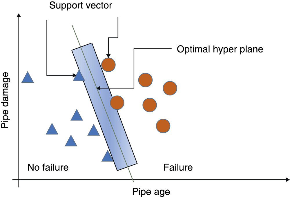
4.3.1.3 Support Vector Machine
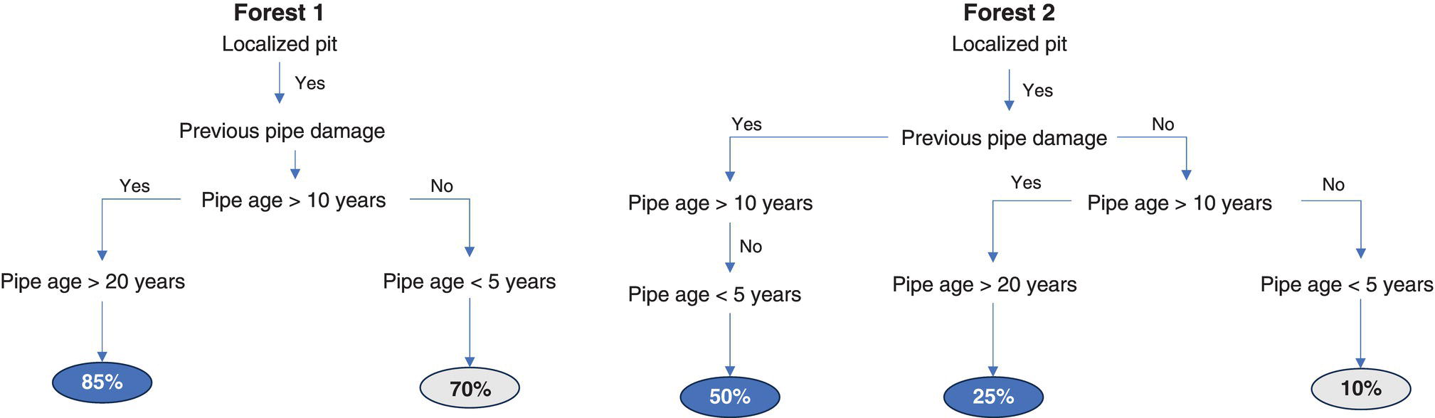
4.3.1.4 Random Forest
4.3.1.5 Gradient Boosting Machine
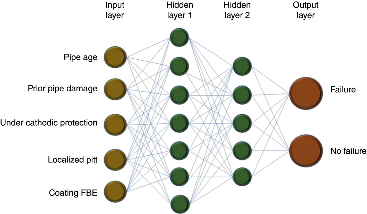
4.3.1.6 Deep Learning Artificial Neural Network
4.4 Problem Example: Predicting Failure by External and Internal Corrosion
4.4.1 Historical Data
4.4.1.1 Feature Engineering
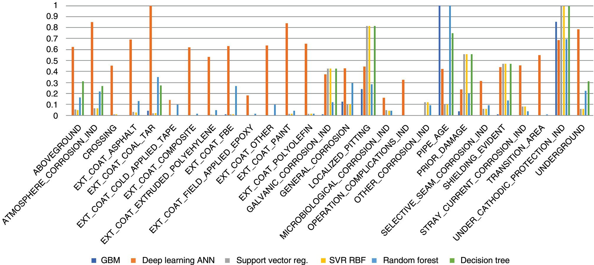
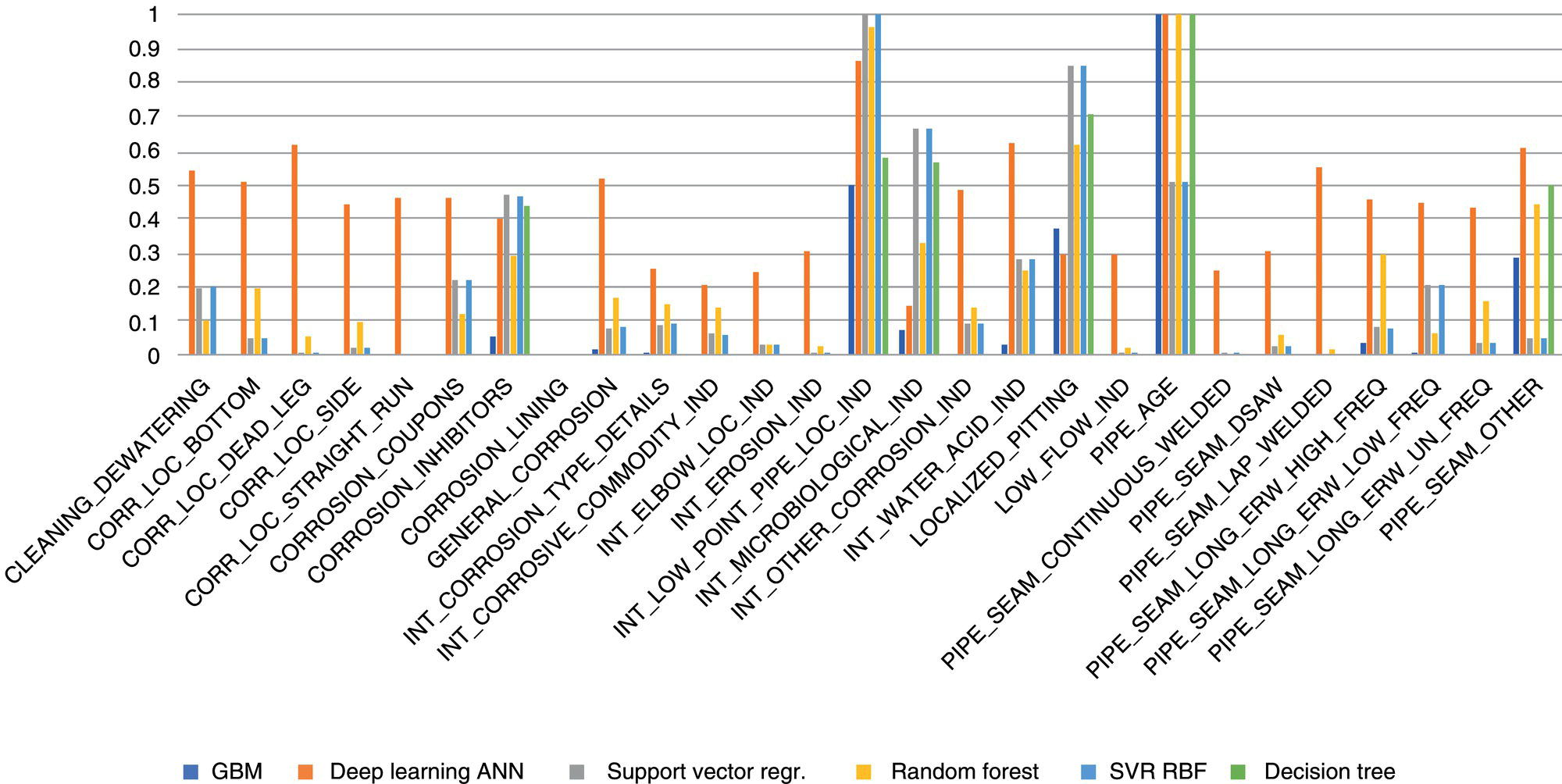
4.4.2 Analysis and Intelligence
Rank
Gradient Boosting
Random Forest
Neural Network
Decision Tree
SVR
1
PIPE_AGE
PIPE_AGE
LOCALIZED_PITTING
UNDER_CATHODIC_PROTECTION_IND
UNDER_CATHODIC_PROTECTION_IND
2
UNDER_CATHODIC_PROTECTION_IND
UNDER_CATHODIC_PROTECTION_IND
EXT_COAT_COAL_TAR
LOCALIZED_PITTING
LOCALIZED_PITTING
3
LOCALIZED_PITTING
EXT_COAT_COAL_TAR
GALVANIC_CORROSION_IND
PIPE_AGE
PRIOR_DAMAGE
4
GENERAL_CORROSION
GENERAL_CORROSION
SELECTIVE_SEAM_CORROSION_IND
PRIOR_DAMAGE
SHIELDING_EVIDENT
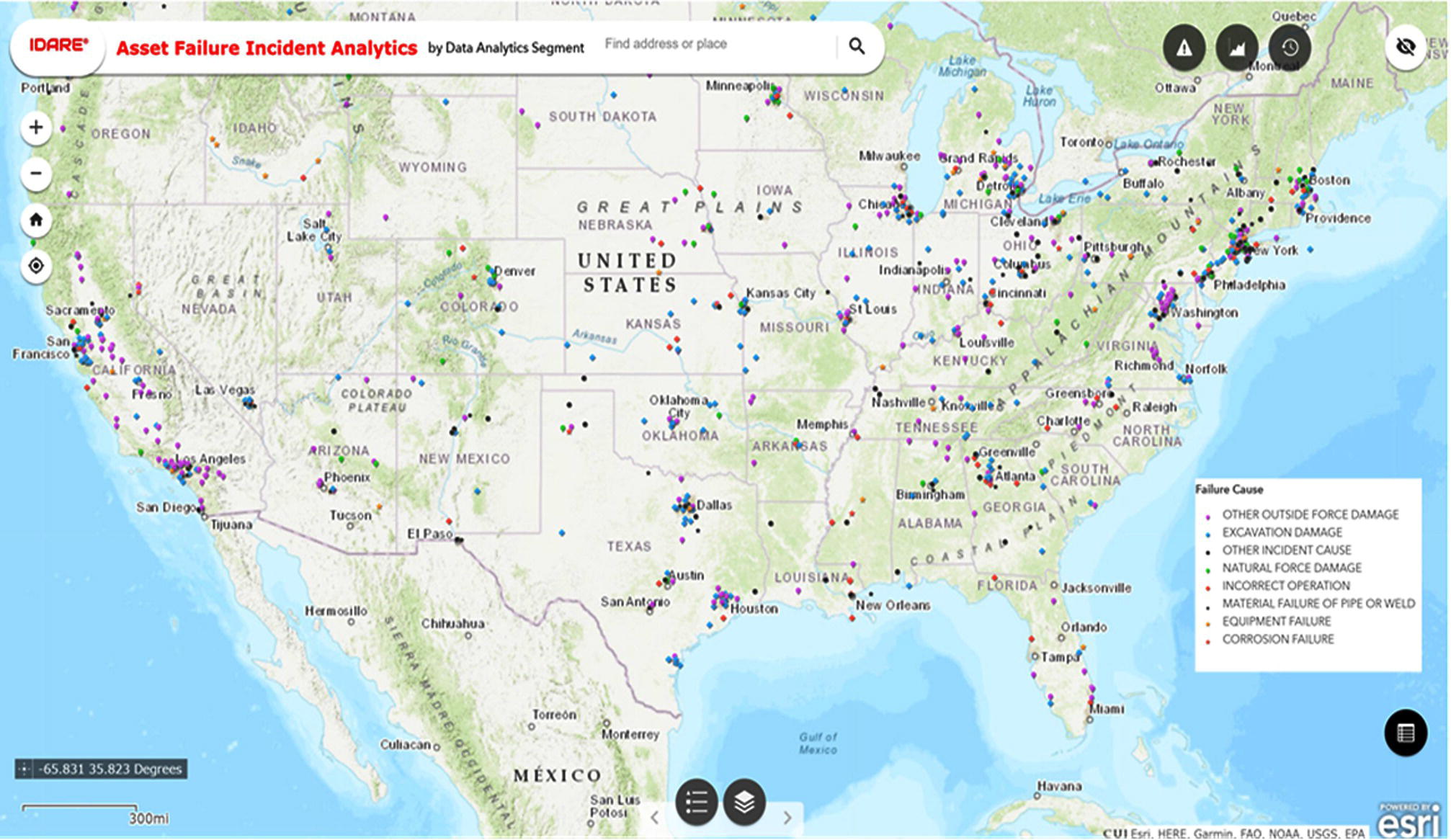
5
EXT_COAT_COAL_TAR
LOCALIZED_PITTING
UNDER_CATHODIC_PROTECTION_IND
SHIELDING_EVIDENT
GALVANIC_CORROSION_IND
Actual
Predicted
Gradient Boosting Machine
Decision Tree
Random Forest
Logistic Regression
Support Vector Machine
Support Vector Machine RBF
Artificial Neural Network
No failure
No failure
37
31
36
37
37
35
35
No failure
Failure
3
9
4
3
3
5
5
Failure
No failure
0
7
0
0
1
0
1
Failure
Failure
85
78
85
85
84
85
84
Total event
125
Accuracy
97.6%
87.2%
96.8%
97.6%
96.8%
96.0%
95.2% 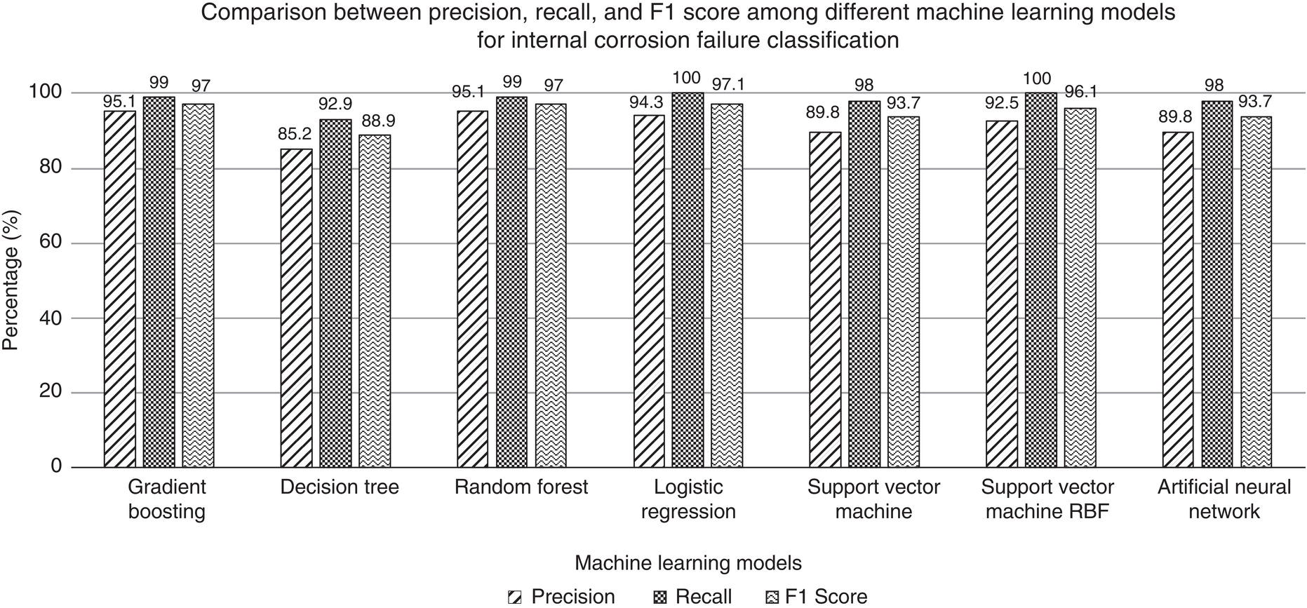
Actual
Predicted
Gradient Boosting Machine
Decision Tree
Random Forest
Logistic Regression
Support Vector Machine
Support Vector Machine RBF
Artificial Neural Network
No failure
No failure
55
56
55
56
56
54
56
No failure
Failure
1
0
1
0
0
2
0
Failure
No failure
1
2
0
1
1
7
0
Failure
Failure
33
32
34
33
33
27
34
Total events
139
Accuracy
97.8%
97.8%
98.9%
98.9%
98.9%
90.0%
100%
Actual
Predicted
Class
No failure
No failure
True negatives
No failure
Failure
False positives
Failure
No failure
False negatives
Failure
Failure
True positives
Actual
Predicted
Gradient Boosting Machine
Decision Tree
Random Forest
Logistic Regression
Support Vector Machine
Support Vector Machine RBF
Artificial Neural Network
No failure
No failure
35
24
35
34
29
32
29
No failure
Failure
5
16
5
6
11
8
11
Failure
No failure
1
7
1
0
2
0
2
Failure
Failure
98
92
98
99
97
99
97
Total event
139
Accuracy
95.7%
83.5%
95.7%
95.7%
90.6%
94.2%
90.6%
Incident Number
Multi Linear
GBM
Linear Regression
RANDOM_FOREST
SVR
DEEP_LEARNING_ANN
SVR_RBF
DT
20200019
Low risk
Low risk
Low risk
Low risk
Medium risk
Low risk
Medium risk
Medium risk
20200025
Medium risk
Low risk
Medium risk
Low risk
Low risk
Medium risk
Low risk
Medium risk
20200031
Low risk
Low risk
Low risk
Low risk
Low risk
Low risk
Medium risk
Medium risk
20200035
Very high risk
Very high risk
Very high risk
Very high risk
Very high risk
Very high risk
High risk
Very high risk
20200037
Very high risk
Medium risk
Very high risk
Very high risk
Very high risk
High risk
High risk
Medium risk
20200051
Low risk
Low risk
Low risk
Low risk
Low risk
Low risk
Medium risk
Medium risk
20200055
Low risk
Low risk
Low risk
Low risk
Low risk
Low risk
Low risk
Medium risk
20200067
Low risk
Low risk
Low risk
Low risk
Low Risk
Low risk
Low risk
Medium Risk
20200070
Low risk
Low risk
Low risk
Low risk
Low risk
Low risk
Medium risk
Medium risk
20200073
Low risk
Low risk
Low risk
Low risk
Low risk
Low risk
Medium risk
Medium risk
20200101
Low risk
Low risk
Low risk
Low risk
Low risk
Low risk
Low risk
Medium risk
20200107
Low risk
Low risk
Low risk
Low risk
Low risk
Low risk
Medium risk
Medium risk
20200110
Low risk
Low risk
Low risk
Low risk
Low risk
Low risk
Low risk
Medium risk
20200112
Low risk
Low risk
Low risk
Low risk
Low risk
Low risk
Medium risk
Medium risk
20200113
Very high risk
Very high risk
Very high risk
Very high risk
Very high risk
Very high risk
Very high risk
Very high risk
20200117
Very high risk
Very high risk
Very high risk
Very high risk
Very high risk
Very high risk
Very high risk
Very high risk
20200120
Very high risk
Very high risk
Very high risk
Very high risk
Very high risk
Very high risk
Very high risk
Very high risk
20200123
Very high risk
Very high risk
Very high risk
Very high risk
Very high risk
Very high risk
High risk
Very high risk
20200125
Very high risk
Very high risk
Very high risk
Very high risk
Very high risk
Very high risk
Very high risk
Very high risk
20200126
Low risk
Low risk
Low risk
Low risk
Low risk
Low risk
Low risk
Medium risk
20200131
Low risk
Low risk
Low risk
Low risk
Low risk
Low risk
Low risk
Medium risk
20200136
Medium risk
Low risk
Medium risk
Low risk
Low risk
Low risk
Medium risk
Medium risk
20200176
Low risk
Low risk
Low risk
Low risk
Low risk
Low risk
Low risk
Medium risk
20200195
Low risk
Low risk
Low risk
Low risk
Low risk
Low risk
Medium risk
Medium risk
20200201
Medium risk
Low risk
Medium risk
Low risk
Low risk
Medium risk
Low risk
Medium risk
20200219
Very high risk
Very high risk
Very high risk
Very high risk
Very high risk
Very high risk
Very high risk
Very high risk
20200236
Low risk
Low risk
Low risk
Low risk
Low risk
Medium risk
Medium risk
Medium risk
20200237
Low risk
Low risk
Low risk
Low risk
Low risk
Low risk
Low risk
Medium risk
20200244
Very high risk
Very high risk
Very High risk
Very high risk
Very high risk
Very high risk
Very high risk
Very high risk
20200249
Medium risk
Low risk
Medium risk
Low risk
Medium risk
Low risk
Medium risk
Medium risk
20200253
Low risk
Low risk
Low risk
Low risk
Low risk
Low risk
Medium risk
Medium risk
20200256
Low risk
Low risk
Low risk
Low risk
Low risk
Low risk
Medium risk
Medium risk
20200272
Very high risk
Very high risk
Very high risk
Very high risk
Very high risk
Very high risk
Very high risk
Very high risk
20200323
Low risk
Low risk
Low risk
Low risk
Low risk
Low risk
Low risk
Medium risk
4.5 Conclusion
Acknowledgments
Abbreviations
ALARP
As Low as Reasonably Practicable
AI-ML
Artificial intelligence machine learning (aka Machine Intelligence MI)
BAST
Best available safe technology
BOL
Bottom of Line, contrast to TOL top of line – both internal mechanisms.
CCT
Critical crevice temperature
CIM
Corrosion and integrity management
CP
Cathodic Protection
CF
Corrosion Fatigue
CRA
Corrosion resistant alloy.
CUE
Corrosion under Excursions (nonsteady, upset, outside design envelope) Related to situational risk.
CUI
Corrosion under insulationb
CUPS
Corrosion under pipe supports
Ecorr
Corrosion potential (Water phase wetted parameter)
FAC
Flow Assisted Corrosionb (Or FILC: Flow Influenced Localized Corrosion)
FSSL
Fail-Safe-Safe-Life (A life cycle integrity KPI)
GHSC
Galvanically induced hydrogen stress cracking.
HSEQ$
Health safety environment quality revenue
HAZ
Heat affected zone.
HE
Hydrogen embrittlement
HIC
Hydrogen induced cracking.
HP/HT/HV
High pressure/high temperature/high velocity.
HRC
Rockwell hardness, C-scale.
HSC
Hydrogen stress cracking.
ISD
Inherently safe design
NDE
Nondestructive examination.
K
Stress intensity factor
K1c
Critical stress intensity factor
KPI
Key performance indicator
PRE
Pitting resistance equivalent
LL
Lessons learned
MIC
Microbially influenced corrosionb
MOC
Management of change
ppm
Parts per million (usually w/w basis).
PINC’s
Prospective (potential) incidents of noncompliance
PWC
Preferential weld corrosionb
PWHT
Post weld heat treatment.
PTVσ
Pressure, temperature, velocity, stress
PHSSSR
Project, health, safety, security, societal, risk (adapted from OilField approach)
RAPP
Re-Appraisal (design review per life cycle degradation)
RBI
Risk-based inspection.
SCCa
Stress corrosion cracking.
SOHICa
Stress-oriented, hydrogen-induced cracking.
SSCa
Sulfide stress cracking.
UDC
Underdeposit corrosion (internal pipe) and equivalent CUD (external pipe)
V&V
Verification (often theoretical) Validation (often practical)
3PR or TPVc
Third-party review (or verification)
References
Pipeline Corrosion Management, Artificial Intelligence, and Machine Learning
(4.1)
(4.2)
(4.3)