Shawn Kenny1 and Paul Jukes2 1Department of Civil and Environmental Engineering, Carleton University, Ottawa, Ontario, Canada 2Pond & Company, The Woodlands, TX, USA Hydrocarbon products, such as oil, natural gas, and natural gas liquids, are transported from the production field to hubs, batteries, tank farms, and facilities via gathering lines or flow lines. Feeder lines or laterals transport the hydrocarbon products to long-distance transmission pipelines that may cross national or international boundaries and extend over tens to hundreds of kilometers in length. In Canada, there is over 100,000 km of transmission line ranging in diameter from 101.6 mm to 1212 mm [1], whereas in the United States, the natural gas transmission pipeline network is more than 480,000 km [2]. These transmission pipeline systems navigate through regions with varied terrain units, topography, physical environment, geology, and, for onshore pipelines, hydrological characteristics. Energy pipelines are typically buried, particularly within urban onshore areas and shallow water offshore regions, to mitigate risk from potential damage due to external force arising from geohazards, natural processes, and anthropogenic activities that may impact mechanical integrity. The external forces are transmitted through the soil and impose geotechnical loads on the buried pipeline. The soil forces and relative soil displacement may be developed through environmental conditions (e.g., soil self-weight and groundwater), operational loading conditions (e.g., pipe self-weight and thermal expansion), anthropogenic activities (e.g., subsidence due to subsurface mining, mechanical damage, and blasting), and natural geohazards (e.g., slope instability, seismic fault movement, and offshore ice gouging). As shown in Figure 13.1, a complex relationship exists between the coupled pipeline/soil system with respect to the demand (i.e., loads and hazards), response (i.e., pipeline/soil interaction, load transfer, and load effects), and capacity (i.e., pipeline mechanical resistance and integrity). As an illustrative example, in the context of ice gouging hazards for offshore pipelines, Kenny et al. [3] present a more detailed discussion on each element within this relationship. For buried pipelines, the system demand (i.e., loads and hazards) is primarily related to anthropogenic activities and natural events. The processes and mechanisms governing system demand are not addressed in this chapter where the technical issues involve complex physics within multidisciplinary fields of expertise. The treatment of external force and geohazards is examined in greater detail within other chapters of this book (e.g., mechanical damage) and other publications [4–19]. For pipelines in frontier regions, such as deep water and Arctic locations, there are unique geohazards that include strudel scour, permafrost-related thaw settlement or frost heave, and offshore ice gouging [20–42]. For small deformation loading events, the system response is primarily governed by equations of equilibrium (i.e., primary loading conditions) with the soil and pipeline system capacity (i.e., mechanical response) dominated by elastic behavior. Current guidelines, codes, and standards provide significant advice on engineering practice to assess the system demand and capacity for stress-based design of pipeline systems [43–49]. Natural geohazards, such as long-term slope movement, landslides, seismic fault movement, and offshore ice gouging, may result in pipelines experiencing large deformations with local plastic strain response that may be associated with mechanisms such as buckling, fracture, and plastic collapse. Laws of compatibility govern the system response and capacity, which is associated with secondary loading events, where limited guidance is provided in current engineering practice [46–49]. These large deformation geohazards drive technology development programs to assess system response and capacity. The development of serviceability and ultimate limit states or other mechanical performance acceptance criteria is not addressed in this chapter with reference to other publications for guidance [3, 38, 41, 50–72]. The consequences of pipeline failure have varying significance that is dependent upon the product type (e.g., oil, natural gas, and gas liquids), pipeline diameter and wall thickness, operating pressure, and location [73–78]. The system demand and system response are not dependent on the product type or consequences and risk level. Figure 13.1 Relationship among system demand, response, and capacity for a buried pipeline system. The response of surficial or partially buried pipelines is an important design element for the offshore environment that has received significant attention over the last decade due to increasing operational pressure and temperature requirements for pipeline transportation systems. The design challenges with pipe/soil interaction and pipe mechanical response have been the subject of research programs and joint industry projects [48, 79–85]. A recent handbook provides a comprehensive overview of the technical issues, reference to supporting publications, and guidance on engineering practice for offshore surface-laid risers and flow lines [33]. Although the key parameters influencing the response of surficial and partially embedded pipeline/soil interaction events have been established, the topic remains an area of current interest and research. These reference publications provide a comprehensive discussion and technical guidance on the subject matter that is not addressed in this chapter. This chapter is specifically focused on the system response elements, as shown in Figure 13.1, for fully buried pipelines. The discussion addresses how engineering tools may be used to estimate the effects of geotechnical loads on buried pipelines (i.e., pipeline/soil interaction, load transfer, and soil failure mechanisms), for long-term ground movement events, and predict the pipeline mechanical response (i.e., geotechnical load effects). Other important factors influencing pipeline/soil interaction events (e.g., effects of loading rate, pore water pressure, and interface behavior) are also highlighted in this discussion. As a prelude to this primary discussion expanded upon later in this chapter, aspects of geotechnical engineering that support pipeline/soil interaction analysis are highlighted in Section 13.2. The use of physical modeling techniques at full scale, large scale, and reduced scale (i.e., centrifuge), which is primarily focused on the soil mechanical response and failure mechanism, is reviewed in Section 13.3.2. A basic understanding of physical modeling techniques is required as this underpins the development and advancement of engineering tools to assess pipeline/soil interaction events and system response. Engineering practice using analytical tools (Section 13.3.3.1) and structural numerical modeling procedures (Section 13.3.3.2) to assess geotechnical load effects on buried pipelines, with reference to current practice documents [43–46], is examined. Further guidance on how to improve the current state of the practice (Section 13.3.3.2) through incremental refinement is presented in Section 13.3.4. An overview of emerging trends in advanced numerical simulation of pipeline/soil interaction events, addressing system response, is provided in Section 13.3.5. Linked with these refinements and advancements, in the computational simulation of pipeline/soil interaction events, is the incorporation of more robust but technically challenging constitutive models that imposes greater requirements on the input data, field programs, laboratory testing, and skill sets for the analysis and interpretation of numerical pipeline/soil interaction simulations. In reference to recent studies, guidance on the application and refinement of common soil constitutive models within this numerical simulation framework is presented in Section 13.3.6. Finally, a high-level outlook on the integration of advancements in the state of the art to become an improved state of the practice is discussed in Section 13.3.7. From this perspective, a key goal of this chapter is to establish a progressive narrative, where as an outcome the reader develops an appreciation and understanding of how the current state of the practice (Section 13.3.3) is in a state of the change that is evolving from an idealized structural modeling basis (e.g., Winkler-type foundation model) toward a more robust and comprehensive technology framework (Sections 8.3.4–8.3.7). The primary motivation was the need to develop advanced engineering solutions that address the conservatism and technical uncertainty in current practice, while satisfying governing constraints (e.g., logistics and economics) for energy pipeline transportation systems in harsh frontier environments, such as deep water and Arctic regions. The integration of conventional geotechnical engineering practices (i.e., field, laboratory, and analysis studies) with recent advances in computational software and hardware platforms has provided this technology framework to improve the state of the practice for assessing geotechnical load effects on buried pipelines. Although current engineering practice continues to principally serve the needs of industry, in this chapter, it is argued that refinements to this technical approach are needed. Advancements in the state of the practice will occur through a technology framework that incorporates laboratory testing, physical modeling, and advanced computational modeling procedures, which are explored in this chapter. The need for advanced user skill sets to pursue this technology path is recognized; however, it is expected that these outcomes from the emerging applied research and development activities will ultimately be formulated within a practical design framework. For example, the approach used to develop the load resistance factored design (LRFD) philosophy used for offshore pipelines and geotechnical structures could be adopted [49, 86–89]. This technology framework and advancement in the current state of the practice will provide industry with a sound technical basis to develop practical engineering solutions with reduced uncertainty and improved confidence in predictable, reliable outcomes. In order to conduct the pipeline system response analysis, the geotechnical conditions along the pipeline route must be established and assessed through site characterization that includes desktop studies, remote sensing, reconnaissance, and field investigations. The current state of the practice integrates data and knowledge from the disciplines of remote sensing, terrain analysis, pipeline routing, geotechnical engineering, and geohazard management to achieve successful engineering design solutions [8, 15–20, 90–96]. A detailed discussion is presented in these cited references, where the primary objectives are to identify the preferred pipeline route that evaluates and balances other factors and constraints that include cost, crossing of water bodies and infrastructure, potential environmental impact, and land use. The pipeline route assessment and selection involves multidisciplinary fields of study that must assess the biological, physical, geophysical, geotechnical, hydrological, and socioeconomic environments. The site characterization and geotechnical engineering studies must be linked with the geophysical and geotechnical surveys in order to establish the engineering parameters for use in analysis and design. The scope and level of detail required is dependent on the pipeline engineering design requirements related to the pipeline location (i.e., onshore, offshore, water or shore crossing, and facility approaches), route length, expected variability in soil conditions, geohazard characteristics (i.e., type, magnitude, and impact), and project-level design philosophy (i.e., stress-based or strain-based design) [96–101]. These activities may also be influenced by other factors related to project execution (e.g., lack of data, uncertainty, and long lead times) and operational strategies (e.g., monitoring, assessing, and mitigating geohazards) [8, 10, 53, 93, 94]. Furthermore, the planning, logistics, work scope, level of detail, resource requirements, and cost increase with the pipeline engineering project gates or phases associated with concept selection, front-end engineering design (FEED), and detailed design activities. In the following subsections, a brief overview of the key factors that influence pipeline routing, site characterization, and geotechnical investigations in support of pipeline system response analysis is reviewed. This discussion highlights the major considerations for conventional or standard pipeline engineering projects and identifies key elements that are required to address specific geohazards and special design considerations (e.g., deep water and northern harsh environments). Reference to other authoritative studies and engineering practice is also provided. Similar to other linear infrastructure in the civil built environment (e.g., highways and transmission lines), geotechnical site characterization and geohazard assessment are integral components of the route planning and selection process and pipeline engineering design activities [8, 10, 15–17, 90, 91, 93, 94, 96–98, 102]. The reader is directed to these comprehensive references for a more detailed discussion on the importance of pipeline route selection for offshore and onshore pipelines and the important connection with geotechnical investigations and geohazard assessment in support of pipeline engineering analysis, design, and construction activities. One of the primary outcomes is to support effective decision-making in pipeline engineering design with respect to safety, economics, and pipeline security and integrity. As discussed by Palmer and King [94], significant technical, logistical, and economic issues can be realized through uninformed or misinformed engineering decision-making based on poor quality or lack of data. In the route planning and selection process, geotechnical site characterization is integrated with knowledge from other scientific disciplines including meteorology, hydrology, surficial geology, seismology, physiography, biology, and zoology, and other factors related to public safety, land use, and sustainability. One of the key issues when selecting an optimal pipeline route is to establish an alignment that mitigates terrain effects and impact of geohazards on pipeline design, construction, and operations within the permitted right of way. Furthermore, the development of construction, operational, and integrity management plans may also be influenced by these geotechnical considerations. For example, the pipeline route may pass through regions with sensitive clays, ground subsidence or acid rock drainage due to mining activities, active slope failures, seismic fault zones and soils with liquefaction potential, limited seasonal access (e.g., muskeg), or permafrost for northern pipelines. Although there are common requirements, onshore and offshore pipeline systems present unique challenges and constraints during surveying and route planning activities that must account for the pipeline life cycle [8, 10, 15–17, 19, 90, 91, 93, 94, 96, 102]. The vast majority of onshore and offshore pipeline systems are resting on the ground (seabed surface) or fully buried with a soil cover above the pipeline crown. The pipeline may be embedded or buried within the soil to address requirements for flow assurance (e.g., thermal resistance), operational loads (e.g., global buckling), and external forces due to wave and current loads (e.g., on-bottom stability), to afford protection from natural hazards (e.g., slope movement, ice gouge events, frost heave, and thaw settlement), outside force (e.g., fishing gear and anchor impact), and third-party damage (e.g., blasting, surface loads, excavators, and farm equipment) [10–42, 44, 46, 79–85, 96, 102]. This section is focused on the geotechnical investigations and data needed to support engineering studies on pipeline system response analysis that are used in pipeline engineering design and integrity assessment. A detailed discussion on the requirements of geotechnical surveys and investigations to support engineering analysis and design is provided in several comprehensive references and recommended practice documents [91, 93, 94, 96, 99–102]. The requirements for planning and conducting the work scope for obtaining the soil parameters used in engineering analysis and design with respect to field investigations, data acquisition and sampling, in situ and laboratory testing, and reporting are examined in detail. The primary geotechnical parameters include the physical and strength parameters for clay or cohesive soil (i.e., particle size distribution, Atterberg limits, unit weight, and undrained shear strength) and sand or noncohesive soil (i.e., particle size distribution, unit weight, relative density, and internal friction angle). For conventional stress-based pipeline design, there is typically limited scope on special considerations in the pipeline routing, site characterization, and geo-technical investigation activities. Conventional engineering practices can be used with successful outcomes realized in the engineering design and pipeline operations [12, 19, 33, 45–47, 49, 99–101]. However, for large deformation, displacement-controlled pipeline response mechanisms (e.g., global buckling and ratcheting) and geohazards (e.g., long-term slope movement, frost heave, thaw settlement, seismic fault movement, liquefaction, and offshore ice gouging), where strain-based design methods are typically used, a more comprehensive geo-technical investigation framework is required [10, 15, 29, 42, 45, 46, 48, 96–102]. For these large deformation geohazards, the type, spatial variability and intensity, and influence on pipeline mechanical response have a significant impact on the need and requirements for site characterization studies and geotechnical investigations in support of pipeline/soil system response analysis. The characterization of geotechnical conditions and assessment of geohazards should not be confined to a focused corridor, such as the pipeline right of way but also assess the surrounding region and terrain units that may affect the pipeline mechanical integrity. A number of factors require thoughtful and practical assessment that will enhance decision making and provide a sound basis for pipeline design, project execution, and operational pipeline integrity management. These factors include an evaluation of the data type (e.g., index properties and laboratory tests), level of detail (e.g., quantity, model or data uncertainty, and spatial variability of soils), and significance of any geohazard (e.g., frequency, system demand, or load intensity) that drive the requirements for geotechnical site characterization and field investigations in support of pipeline engineering design activities. The importance of geotechnical investigations for defining the geotechnical and geophysical attributes for use in conducting pipeline analysis and design, such as soil type, mechanical properties (e.g., cohesion and friction angle), groundwater conditions (e.g., spatial and seasonal variation), and unique features (e.g., bedrock, aggressive chemicals, and geohazards), cannot be understated. The ultimate goal is to provide baseline data for conducting physical tests or numerical simulation to assess the geotechnical load effects on buried pipelines and predict the pipeline mechanical response. Over the past 50 years, the technical engineering approaches to assess pipeline/soil interaction events have evolved from empirical observations and idealized closed-form solutions through to a suite of advanced numerical simulation techniques. The primary goal is to estimate load effects on pipeline mechanical performance in support of engineering design and operational integrity. The advanced computational engineering tools provide a technically robust and cost-effective framework to conduct detailed investigations on pipeline mechanical response to pipeline/soil interaction events across a range of practical design parameters. These engineering tools, however, are fundamentally dependent on input data from engineering surveys to define the pipeline alignment and profile, field programs to collect route specific geotechnical conditions, laboratory tests to define parameters used in constitutive models of the engineering computational tools, and physical models to provide confidence in these numerical simulation tools. In this chapter, components of this integrated technology framework in support of pipeline engineering design are addressed in terms of an overview of the current state of the practice, evaluation of the technical requirements, advantages and constraints for each technology approach, and an assessment of the current state of the art. A physical model is typically a smaller physical copy of an object. The geometry of the model and the object it represents are often similar in the sense that one is a rescaling of the other. Similarity of pipe/soil interaction models is also required in terms of mechanical response. Mechanical and geotechnical similarity can be considered using dimension-less analysis to ensure that physical models are representative [103–105]. In other subsections within this chapter, the contributions of physical modeling studies, investigating the soil mechanical response and pipe/soil interaction mechanisms, with respect to the development of current knowledge base, formulation of existing industry practice and guidance documents, and foundation for areas of emerging research are referenced and discussed. Examples of simple elemental lateral, vertical, or axial pipe/soil interaction events, with a rigid pipe segment, are examined. The importance for integrating physical modeling studies to develop practical engineering tools in support of pipeline design, and to establish confidence in more advanced computational modeling procedures, addressing state-of-the-art pipe/soil interaction studies, is presented. For example, the historical literature indicates that the drained lateral interaction load factors for noncohesive soils, based on physical model tests, may differ significantly. Recent studies have shown that these differences can be explained by consideration of the pipe size and contribution of soil self-weight to the soil mechanical resistance. The importance of effective stress level in soil response is also an essential consideration. These issues are discussed in further detail later in this chapter. Furthermore, physical models of larger pipeline/soil interaction systems examining large-scale ground movement events, such as ice gouging, seismic fault movement, and frost heave mitigation, have provided important insight and are referenced in the discussion. For pipeline/soil interaction events when soil weight effects are important, physical modeling tests are best conducted under large, near full-scale, field-scale conditions or in reduced-scale models using a geotechnical centrifuge. There are at least three large-scale geotechnical physical modeling facilities in North America focused on pipeline testing at Queen’s University, Cornell University, and University of British Columbia [106–111]. There are a larger number of geotechnical centrifuge modeling centers with more than 100 facilities operating worldwide [33, 112, 113] with the principles of geotechnical centrifuge modeling effectively summarized in several publications [33, 114]. Physical modeling is most beneficial when complemented by other engineering studies within an integrated framework that includes field investigations, laboratory testing, and computational simulation. These concepts are reinforced in the following subsections where excellent comparisons between physical modeling and numerical simulation of pipe/soil interaction events are discussed and referenced. Analytical solutions characterizing the mechanical response of surface-laid and buried pipelines have generally evolved from the concept of a subgrade reaction [115]. The Winkler model was initially developed to examine rail/ground surface interaction problems through a linear solution relating the foundation pressure with the foundation modulus and deflection. The foundation was modeled as a series of independent or decoupled, discrete springs with specified stiffness. The Winkler model was extended through multiparameter models that accounted for the beam and soil behavior [116–121]. As discussed by Konuk et al. [120], the parameters for multiparameter models are established through knowledge of the corresponding solution to the applicable continuum problem. These structural-type models introduce simplifying assumptions, idealizations, and constraints with respect to the spatial distribution of the displacement and stress fields, which may not necessarily produce conservative results [121–124]. There exists a range of simple empirical and closed-form solutions to estimate geotechnical loads on buried pipeline [44, 46, 125–132]. These methods are constrained by the governing idealizations but provide a relatively simple engineering tool for use in preliminary engineering design iterations and as a confidence check for more rigorous and complex analysis. The engineering tools and key design parameters derived were generally associated with an assessment of the limit load as defined by the ultimate soil load capacity and yield displacement. Using numerical techniques such as finite difference and finite element methods, the Winkler model was extended to more complex, nonlinear problems with large deformations, such as the analysis of buried pipeline/soil interaction events. Engineering guidelines for the analysis of buried pipeline/soil interaction events were developed in the 1980s and have been refined through advances in research [12, 43, 45, 46]. These engineering guidelines model the pipe/soil system as a series of connected structural beam and spring elements (Figure 13.2). The analysis techniques have evolved and engineering tools have been applied to the analysis of fault movement due to seismic events, ground settlement, upheaval and lateral buckling instability, ice gouging, frost heave and thaw settlement, and riser touchdown [3, 26, 120, 133–138]. Figure 13.2 Schematic illustration of the (a) continuum pipe/soil interaction problem and (b) mechanical idealization using beam and spring structural elements. This subsection provides an overview of pipe/soil interaction models for buried pipeline systems for conventional pipeline engineering design considerations in the onshore and offshore domains. The examination of special topics, such as Arctic pipelines and surficial pipeline systems, is presented in Section 13.4. Euler-Bernoulli or Timoshenko beam theory defines the beam element behavior that may also have additional variables to account for the effects of internal pressure, thermal expansion, section ovalization and warping, and stiffness or flexibility characteristics for curved sections or elbows. The pipeline constitutive model is generally defined as isotropic, elastoplastic behavior with piecewise representation of the stress–strain relationship. The pipe plastic material response is generally defined by the von Mises yield surface with isotropic hardening rule [139, 140]. The plasticity models may also need to account for kinematic hardening, which is important for cyclic loading problems such as fatigue, ratcheting, and offshore reel-lay installation [141–143]. The soil continuum response is idealized through a series of discrete springs, which represent the generalized mechanical response of a segmented soil slice, connected to the pipe. The spring elements represent the soil force–displacement response per unit length of pipe that act on three mutually orthogonal axes to the pipeline centerline defined along the longitudinal, transverse horizontal, and transverse vertical directions. The soil spring force–displacement relationships are defined by engineering guidelines [43, 45, 46] with bilinear (i.e., elastic-perfectly plastic), piecewise multilinear, or hyperbolic functions to represent the nonlinear response characteristics. The soil spring load–displacement relationships define the ultimate load and yield displacement through geometric properties (i.e., pipe diameter and pipe springline depth), soil physical properties (e.g., adhesion, soil unit weight, and pipe/soil interface friction angle), soil strength properties (i.e., cohesion and internal friction angle), and interaction factor (i.e., bearing capacity factors). The soil spring parameters, such as yield load, yield displacement, and empirical coefficients for bearing interaction, have been primarily established through scaled physical modeling studies in uniform soil conditions [144–149]. Although it is recognized that the postpeak residual force may be less than the ultimate soil load that may be associated with strain softening mechanisms, the guidelines generally consider a constant postpeak soil force. The loading and unloading response of the soil springs traces along the same force–displacement relationship. In the following sections, the basis for soil spring formulation in the longitudinal, transverse lateral, and transverse vertical directions is examined and critiqued. Guidance on the state of the practice and state of the art in support of pipeline engineering design is discussed in Section 13.3.4. The development of emerging engineering tools for pipeline/soil interaction analysis, through research and development studies, that may advance current practice is explored in Section 13.3.5. In the following subsections, a mixed formulation is used to characterize the soil ultimate force (tu, pu, quu, and qud) as a function of strength parameters, as recommended by the industry guidance documents [43, 45, 46] for simple axial, lateral, or vertical pipe/soil interaction load events. The mixed formulation includes total stress (α-method) and effective stress (β-method) approaches. From the author’s viewpoint, the use of mixed formulation to define the soil mechanical response is not recommended. The use of effective stress formulation to represent soil mechanical response and characterize pipe/soil interaction events is recommended and considered more representative of soil behavior during pipeline/soil interaction events [14, 108–111, 148–157]. The β-method can account for undrained and partially drained loading conditions when the excess pore pressure is known or estimated. For example, in saturated cohesive soils, the friction angle is typically small (i.e., <5°); however, as the water content is decreased, the importance of the friction angle on strength mobilization will increase for the same adhesion resistance [8]. Estimates on soil axial forces were established using pile theory where the limit skin friction per unit area (fs) at the pipeline/soil interface can be expressed by the α-method (i.e., total stress response) as [150] and by the β-method (i.e., effective stress response) as The engineering guidelines [45, 46] provide a mixed formulation (i.e., combining total stress and effective stress concepts) defining the ultimate or maximum longitudinal soil force as The ultimate soil displacement is defined as 8–10 mm for stiff to soft clay and 3–5 mm for dense to loose sand [45, 46]. The axial soil load–displacement relationship is generally defined as bilinear, elastic-perfectly plastic response. The adhesion factor (α) can be estimated through back calculation from pile load tests for undrained loading conditions. In pipeline engineering design, however, drained conditions are typically assumed for axial loading events [145, 150–152]. Except for fast loading conditions (e.g., seismic fault movement and liquefaction), it is expected during axial pipe/soil interaction events that the excess pore pressures, generated by shear stress, will rapidly dissipate through a thin soil layer circumscribing the outside pipe diameter. This would result in a drained loading condition that requires effective stress analysis. For the axial response, using one-dimensional consolidation theory, the effects of load duration on drained versus undrained behavior can be assessed using the degree of consolidation at specified depth and time [151]. Although methods exist to correlate the adhesion factor and undrained shear strength (su) with effective stress state [152], other factors influence the undrained shear strength soil for pipe/soil interaction events that include soil sensitivity, strain rate effects, and reduction in the soil water content with increased pore water suction, consolidation, soil desiccation, and cementation. These factors (i.e., displacement rate effects, water content, and consolidation) may only partly account for the uncertainty and significant scatter in the adhesion values as proposed by the ALA guidelines [46]. Experimental studies and well-controlled full-scale field tests indicate significantly lower values for the adhesion factor [150, 153, 154, 158]. In addition, recent studies have indicated that slight axial misalignment (i.e., oblique pipe/soil interaction) or pipe asperity (e.g., larger diameter transition and inline valve) can increase the longitudinal soil resistance [113, 159, 160]. However, displacement rate effects may also play a role in the differences between the adhesion factors as discussed by industry guidelines [43, 45, 46]. The validity of adopting the α-method from pile theory for application to buried pipeline systems for both cohesive and noncohesive (frictional) soils, however, remains an open question [150, 154]. For pipeline designs incorporating the α-method to estimate longitudinal soil resistance, higher adhesion factors should be selected when the maximum longitudinal soil forces are important for pipe stress (e.g., von Mises stress) and stability (e.g., global buckling) analysis, whereas lower adhesion factor should be selected to determine soil strength (e.g., virtual anchor lengths for thermal expansion analysis). The effective stress parameter (β-method) is influenced by the effective normal stress state and pipe/soil interface friction angle (δ), which can vary from 0.5ϕ′ to 1.0ϕ′, and is dependent on the characteristics of the external pipe coating and surrounding soil [3, 45, 145, 161]. These friction angle estimates, however, do not account for the effects of damage, degradation, or long-term creep response of the external pipe coating material [154]. Based on direct shear box tests and comparison with field trials, axial pipe frictional load magnitude was governed by characteristics of the external pipe coating roughness and compliance with limited effect from the soil backfill conditions [150]. Pipeline coatings with a smooth and hard surface will minimize axial loads for both cohesive and noncohesive (frictional) soils. For offshore pipelines in noncohesive soil, the interface friction angle (δ) can be estimated as [152] For cohesive soils with drained loading conditions, the peak interface friction angle can be estimated as The axial soil load is also significantly influenced by the lateral earth pressure coefficient at rest (K0). The ALA and PRCI guidelines [45, 46] do not provide any recommendation on the value, but a value of 0.5 is typical with the general expression K0 = 1 − sin ϕ′ recommended. Further discussion on the determination of the lateral earth pressure coefficient at rest is presented in Section 13.3.6.2. The lateral earth pressure coefficient at rest accounts for the general stress state at the pipe springline and does not account for the actual stress state or local deformations during the pipe/soil interaction event. For loose sand conditions, axial pullout tests are consistent with industry guidelines [43, 45, 46] as expressed in Equation (3.3). In dense sand, however, the measured axial loads were significantly greater than the recommended guidelines where increased resistance was due to constrained dilation, in response to shear deformation, within a thin annular zone circumscribing the pipeline [108–111, 150, 154, 156–158, 162]. For larger diameter pipeline, the NEN 3650 [43] guideline states that the pipe self-weight and contents should also be considered when determining frictional forces during axial pipe/soil interaction events. The use of hard and smooth coatings was recommended to mitigate pipe/soil interface friction and axial loads irrespective of the soil conditions [157]. Based on the bilinear model, the maximum transverse lateral soil force per unit length of pipe segment is expressed as [45, 46] Estimates of the maximum transverse lateral soil force have been established through analytical solutions (e.g., passive earth pressure theory and strip footings), physical models (e.g., anchor plates, piles, and pipe), and numerical simulation (e.g., finite element analysis of anchors and pipe) [108, 111, 145, 146, 148, 149, 156, 160, 163–189]. For slow loading rates in cohesive material, effective soil strength parameters for noncohesive soil (e.g., sand) can be used to predict the lateral load–displacement response in cohesive soil (e.g., clay) [148, 158, 190]. The ultimate soil displacement at the peak transverse lateral soil load is expressed as a function of the pipe burial depth [45, 46]: The force–deflection relationship for lateral pipe/soil interaction events exhibits nonlinear response characteristics with strain hardening or strain softening behavior. The soil spring force–deflection relationship can be represented using bilinear, elastic-perfectly plastic behavior or hyperbolic functions through piecewise approximation [148, 149, 165, 171, 191–194]. Project-specific data including the results from physical tests or numerical simulations may also be used to establish the soil load–displacement relationship. Interpretation of the soil load–deflection response and establishing the maximum transverse lateral load and corresponding soil displacement at the peak load on a consistent basis are required. This can be achieved through definition of rational selection criteria. These criteria are established in reference to the characteristic shape of the soil load–deflection response that include (1) peak load associated with a unique maximum (e.g., classical strain softening response) or asymptote (e.g., classical strain hardening), (2) intersection of a tangent line to the strain hardening response with the ordinate, (3) intersection of tangent lines to the elastic modulus and strain hardening response, (4) secant line with a slope equal to one-quarter of the elastic modulus (k4 method), and (5) secant line with an upper load limit fraction (0.70–0.95) of the maximum peak load [167–169, 171, 191–196]. Transverse lateral pipe/soil load events involve complex interactions with dependence on parameters that include soil strength characteristics (e.g., undrained shear strength, consolidation ratio, and internal friction angle), burial depth, loading or displacement rate (i.e., drained or undrained conditions), large deformation soil behavior (e.g., strain hardening, strain softening, and dilation), interaction and contact processes (e.g., trailing edge separation or breakaway, negative or suction pressure, and infilling), trench effects (e.g., backfill properties and trench geometry), and failure mechanisms (i.e., plastic wedge formation with uplift at shallow burial depth and local punching failure with flow at deeper burial depth). These parameters will influence the maximum load, displacement at peak load, and interaction factors. The interaction factor (Nch) for cohesive soil, as defined by industry guidelines [43, 45, 46], is generally based on the work of Hansen [165], assuming undrained conditions (i.e., total stress analysis). Several studies have demonstrated the importance of loading rate, associated with time-dependent consolidation of cohesive soils, on the lateral interaction loads [113, 148, 190]. As shown in Figure 13.3, for rapid loading events, where undrained conditions prevail, the interaction factors were consistent with the immediate separation (breakaway) results of Rowe and Davis [171] but less than the estimates based on the approach by Hansen [165]. These observations are consistent with the findings of Popescu et al. [179] for physical and numerical models of pipe/soil interaction in soft and stiff clay. For slower loading rates, where drained conditions and effective stress state become more prevalent, the current state of the practice, based on total stress analysis, underestimates the load transfer to the pipe [148, 190]. Recent studies have also indicated the importance of burial depth, soil weight, and failure mechanism on the lateral bearing interaction factor [113, 190, 195–197]. Through continuum finite element simulations, the predicted transverse lateral bearing interaction factor (Nch) was consistent with the study by Hansen [165]. The key finding from these studies, however, was the contribution of the soil weight to the interaction factor for shallow buried pipelines associated with a passive wedge failure mechanism. Based on the work of Rowe and Davis [171], Phillips et al. [113] proposed a modified interaction relationship that accounted for the effects of soil weight within the passive wedge: Figure 13.3 Vertical bearing downward interaction factors. A total stress analysis was conducted with undrained conditions assumed and effective stress parameters defined at the pipe/soil interface. The coefficient β relates the effect of the soil weight relative to the vertical stress at the pipe springline and normalized with the soil undrained shear strength. The numerical studies [113, 195–197] indicate that the significance of the coefficient β diminishes at pipe springline burial depth to pipe diameter ratios (Hs/D) greater than 5, which is related to the transition in the governing failure mechanism. The coefficient β was defined as a constant value of 0.85 [113], but recent numerical modeling studies [195–197] suggest that the coefficient may be a function of the pipeline burial depth and intensity of equivalent plastic strain within the failure zone. The upper limit for the bearing factor ( For noncohesive soil, the interaction factor (Nqh), as defined by industry guidelines [43, 45, 46], is based on the work of Hansen [165] that increases with increasing burial depth ratio (Hs/D) and soil internal friction angle across the range of 20–45°. The studies by Neely et al. [167], Audibert and Nyman [168], and Popescu et al. [179] were consistent with industry guideline [43, 45, 46] estimates of the lateral bearing interaction factor for noncohesive soil. Other studies predict a reduction in the lateral bearing interaction factor by a multiplier of 0.5–0.67 [148, 172, 198, 199]. Recent studies have reconciled this issue through accounting for the effects of pipe size and soil weight [113, 138, 160, 183, 197, 200–202]. Further studies are required to provide reliable estimates of the lateral bearing factor in partially saturated noncohesive soil conditions due to the complex relationship with soil shear strength, dilation, deformation response, and failure mechanisms. In contrast to the axial and lateral soil load–displacement behavior, the vertical downward bearing and uplift response mechanisms can be characterized as asymmetric for most pipeline design burial depths. The soil load–displacement relationships account for the differences in stiffness, yield displacement, and yield load for the respective directions. The maximum transverse vertical uplift soil force per unit length of pipe segment is expressed as [45, 46] The vertical uplift soil load–displacement relationship is based on theoretical solutions, physical tests, and finite element analysis [146, 171, 172, 203]. Over the past decade, there has been significant number of studies examining the uplift behavior of partially or fully buried pipelines with respect to global instability mechanisms due to upheaval buckling [149]. The following discussion is focused on static pipe/soil interaction events that are stable from the kinematic perspective. For cohesive soil, the vertical uplift bearing factor (Ncv) was based on the theoretical solution for buried cylinders by Vesic [203], adopted by Audibert et al. [204], and is considered valid for springline depth ratios (H/D) less than 10. The vertical uplift bearing factor is bounded by finite element analysis of horizontal plate anchor with assumed immediate breakout (slip) and fully bonded conditions [45, 46]: In noncohesive soil, the vertical uplift bearing factor (Nqv) was based on physical modeling of buried pipelines and numerical simulation of horizontal plates [146, 172]: where the overburden bearing capacity factor (Nq) was based on Meyerhof [205] bearing capacity factor defined as The ultimate yield displacement is defined as for stiff to soft cohesive material and for dense to loose noncohesive soil. The vertical downward soil load–displacement relationship can be established using bearing capacity theory based on Meyerhof [205]. The relationship between soil friction angle and the overburden (Nq), cohesion (Nc), and failure wedge bearing interaction factor (Nγ) is illustrated in Figure 13.3. The maximum transverse vertical uplift soil force per unit length of pipe segment is expressed as [45, 46] The soil cohesion bearing interaction factor (Nc) is defined as where Nc = 5.14 in the limit with an internal soil friction angle of 0°. The failure wedge bearing interaction factor (Nγ) is defined as The ultimate yield displacement (Δqd) is defined as 0.2D for cohesive soil and 0.1D for noncohesive soil. Modeling is an inherent characteristic and fundamental component for engineering analysis and problem solving. Over the past 30 years, there has been significant advancement in computational hardware and software technology that has provided a technically robust, efficient, and cost-effective tool for the numerical simulation of geotechnical engineering problems including pipeline/soil interaction. The technology framework relies on laboratory tests to support the development and refinement of constitutive models and physical modeling to calibrate and verify the numerical modeling procedures [8, 33, 92, 95, 105, 206–211]. Field investigations are conducted to provide focus for these specialized studies in support of engineering design activities in order to develop practical engineering solutions. In Section 13.3.3, the state of the practice for pipeline/soil interaction analysis using structure-based modeling techniques was presented. In the following sections, engineering guidance on the use of structure- and continuum-based finite element modeling procedures for pipeline/soil interaction analysis is presented. The motivation for this discussion is to provide an overview of the inherent limitations, constraints, advantages, and future trends for each technical approach. A discussion on physical modeling studies, for research and in support of engineering design, with respect to pipeline/soil interaction events was presented in Section 13.3.2. The current state of the practice for pipeline/soil interaction analysis using structure-based numerical tools, through beam and spring elements to idealize the continuum response (Section 13.3.3.2), has served industry needs for the past three decades. Pipeline/soil interaction problems, such as fault movement due to seismic events, ground settlement, upheaval and lateral buckling instability, ice gouging, frost heave and thaw settlement, and riser touchdown, have been examined using these structural pipe/soil interaction simulation tools [14, 26, 51, 120, 127, 128, 134–137, 212–216]. In comparison with other numerical techniques, such as continuum-based finite element methods (discussed in Section 13.3.7), structure-based tools require a relatively lower degree of technical proficiency in numerical modeling, limited computational hardware resources, and less computational time for equivalent pipeline systems being analyzed. However, there exists uncertainty on the adequacy and reliability of these structure-based pipeline/soil interaction tools particularly with respect to large deformation ground movement events that may have nonmonotonic loading path or complex boundary conditions. Key factors that support this statement are highlighted in the following subsections. A primary criticism of the structural beam/spring models is the idealization of a continuum with discrete elements that represent the generalized or composite soil mechanical response. This structure-based idealization cannot provide an adequate characterization of more realistic soil mechanical response including load coupling between mutually orthogonal axes, strength behavior with respect to path dependence, pore pressure effects and strain softening and hardening, and shear-induced dilation and compaction. Some of these issues are further explored in the following subsections. The soil load–displacement relationships may be defined by bilinear, multilinear, or hyperbolic mathematical formulations with guidance provided by engineering practice documents [43, 45, 46]. The peak soil loads should be defined in terms of total stress or effective stress formulation. The criterion specifying how the peak load and corresponding yield displacement magnitude should be determined will influence the soil stiffness response [167–169, 193–197]. In general, the multilinear and hyperbolic formulations will have greater stiffness (i.e., less compliance) for subyield loading events than the bilinear counterpart. Furthermore, the hyperbolic formulation may be more representative of the constitutive behavior for soft clay and loose sand but may not provide an adequate characterization of the constitutive behavior for strain softening materials such as dense sand or stiff clay. In general, the spring formulations assume that homogenous soil conditions prevail and do not account for the trench boundary conditions and potential interaction between the pipeline within the trench backfill and the surrounding native soil. Several studies have demonstrated that the pipe diameter, pipe burial depth, trench geometry, and relative soil strength differences (i.e., between the native and backfill soils) will influence the development of peak loads, yield displacement, and failure mechanisms [111, 113, 130, 156, 217–219]. Structural beam/spring models can be tailored to simulate soil backfill and trench wall effects but only within a generalized framework or case-specific application. These idealized numerical procedures, however, cannot account for complex interactions and failure mechanisms that may occur at multimaterial interfaces such as the pipe/soil, trench boundary, or other physical barrier (e.g., geotextile). The use of physical modeling and numerical simulation techniques is needed to address these issues. The pipeline engineer will need to assess all possible design options to mitigate load effects on buried pipelines that may include engineered backfill with optimal trench configurations, preferential route alignment, low friction coatings, and geotextiles. Consideration and optimization of issues such as logistics, project execution risk, and cost will be required. There is general agreement on the general characteristics and parameters influencing the interaction factor, which include pipe diameter, pipe burial depth, soil strength, and pipe/soil interface friction factor. As discussed in Section 13.3.3.2, the interaction (i.e., bearing) factors have been derived through analytical solutions, physical models, and numerical simulations for analog problems (e.g., plate anchor) and buried rigid pipes. Although current practice has served industry needs, some assumptions and technical approaches should be reconsidered where inherent uncertainty can be addressed, leading to more reliable and predictable outcomes. Some of the key factors include the basis for the interaction factors, soil stress state (i.e., total versus effective stress conditions), pipe size and soil stress effects, local pipe/soil interface effects, and soil failure mechanisms. An overview of these factors is presented in the following paragraphs. Axial pipe/soil interaction is dominated by the interaction, load transfer, and failure mechanism developed at the local annular pipe interface with the soil. The interface behavior can be characterized by nonlinear deformation, shear-induced volume change, and excess pore pressure for undrained conditions [108–111, 132, 156, 157, 160, 200, 220]. For cohesive soil, assuming total stress analysis with undrained conditions, these effects are averaged or smeared through the use of an adhesion factor (Section 13.3.3.2). However, there is significant variation in the adhesion factor, as shown in Figure 13.4 [45, 46, 221], that may be attributed to test conditions, misalignment of the pipe axis from pure axial motion, and soil desiccation and cementation [132, 148, 149, 153, 158, 221]. For the pipeline engineer, consideration of the soil type, groundwater conditions, load obliquity, and loading rates is needed when interpreting the adhesion factor. In dense noncohesive soil, recent studies have shown that the axial resistance may significantly increase due to constrained dilation that is underestimated by current pipeline/soil interaction guidelines [108–111, 150, 154, 158]. The use of an effective stress formulation with frictional properties defining the pipe/soil interface may be more representative of longitudinal interface behavior and load transfer mechanisms [149–152, 154, 156, 157, 221–223]. Figure 13.4 Variation of adhesion factor with undrained shear strength. Figure 13.5 Interaction factors for transverse lateral pipe/soil loading events in (a) cohesive soil and (b) noncohesive soil. Recent studies have identified areas of uncertainty with the determination of lateral bearing factor (Nqh) [148, 160, 183, 196, 197]. For example, the test results reported by Trautman and O’Rourke [145, 147] are consistent with the predictions by Ovesen [198, 199] but may differ by a factor of 2 when compared with the tests by Audibert and Nyman [144], which are consistent with the model by Hansen [165]. This variability is illustrated in Figure 13.5 and may be attributed to the soil conditions (i.e., gradation, density, and friction angle), experimental procedures (e.g., data acquisition and reporting and loading rate), and boundary conditions (i.e., plate anchor versus pipe). Recent studies have attributed the differences to the effects of pipe size, soil weight, and failure mechanism [113, 138, 160, 183, 197, 200–202]. For practical range of diameters for energy pipelines, however, the scale effect, as discussed by Guo and Stolle [183], on lateral soil bearing resistance is negligible for diameters greater than 273 mm. Furthermore, as discussed in Section 13.3.3.2, for shallow burial depths, the soil weight being lifted through the lateral pipe/soil interaction has been shown to be a significant parameter on soil resistance that is associated with a passive wedge failure mechanism [113, 195–197, 340]. For deeper pipe burial depths, the failure mechanisms can be characterized by plastic flow around the pipe circumference. Uplift resistance models have generally been developed to establish peak load and mobilization distance parameters for monotonic loading conditions. A significant volume of work has been conducted on vertical uplift resistance for offshore pipelines to mitigate the effects of upheaval buckling mechanisms [48, 83, 104, 213, 222–234, 341, 342]. A complex relationship exists between key design parameters, including pipe (e.g., diameter, weight, burial depth, and interface friction) and soil (e.g., type, gradation, soil state, strength, and dilation) characteristics, with the interaction factor and mobilization distance. These parameters also influence the failure mechanism developed during the pipe/soil interaction event that may be characterized by wedge failure (vertical or inclined) with slip lines or plastic flow model. As the pipeline lifts upward, the soil may fill the void located at the pipe invert and haunches. For pipeline systems with cyclic operational loading conditions (e.g., start-up, shutdown, and restart) or variable operational parameters (e.g., transient pressure), this may result in the continued vertical upward movement of the pipe through a geotechnical ratcheting mechanism [48, 83, 149, 230–234]. In response to the operational loads and out-of-straightness imperfections, the pipe lifts vertically and, in weak cohesive or loose noncohesive soil conditions, the soil may fill the void beneath the pipe. This action prevents the pipe from returning to the initial position and results in the systematic upward creep or ratcheting of the pipe vertically through the soil column. This may lead to a sufficient loss of soil cover that results in pipe global buckling response. These recent studies have provided guidance on upheaval buckling with respect to predicting uplift resistance and mobilization distance, and the significance of geotechnical ratcheting mechanisms. As discussed in Section 13.3.3.2, conventional engineering practice for the analysis of pipeline/soil interaction events is generally performed using decoupled, structural beam/spring models. However, for pipelines subjected to multiaxial loads [235, 236] and foundations subjected to oblique or inclined loads [237–244], a coupled mechanical response along principal directions has been observed. A schematic illustration of oblique loading scenarios in three orthogonal planes is shown in Figure 13.6. The integration of shear coupling between soil springs has also been examined in past studies [123–125, 137]. As previously discussed, these structure-based parameter models (i.e., Winkler-type foundation) cannot account for the complex soil mechanical response with respect to strength evolution (e.g., peak stress, residual stress, and dilation), load and stress path dependence, and deformation mechanisms and strain localization effects. Figure 13.6 Definition of relative attack angles for oblique loading in (a) vertical–axial plane, (b) vertical–lateral plane, and (c) lateral–axial plane. One of the primary goals for investigating load coupling effects during oblique pipeline/soil interaction events is to improve the current basis of the structural beam/spring models. As discussed in Section 13.3.3.2, structural models provide a relatively simple and cost-effective tool that is well suited for pipeline/soil interaction studies involving a large parameter matrix or probabilistic framework [3, 26, 30, 245]. For these problems, the use of more robust computational tools, such as continuum finite element methods, would be limited to a select number of design cases that must be identified through screening analysis with specified assessment criteria. There exists uncertainty, however, on the use of this idealized structural model to simulate complex stress paths, load transfer processes, and failure mechanisms for problems with severe nonlinear behavior involving contact and strain localization [3, 120, 133, 216, 246]. Enhanced structural models can be developed using macroelements or refined spring elements that account for the effects of mechanical load and displacement coupling [138, 247, 248]. These coupled formulations define the soil yield envelope, in terms of the peak load and yield displacement within the three orthogonal planes (i.e., vertical–axial, lateral–axial, and vertical–lateral). Load coupling effects are incorporated within the soil spring formulation through knowledge on the shape of the peak load and yield displacement failure envelopes for specific design conditions, such as pipe diameter, pipe burial depth, soil type and strength properties, and attack angle. For macroelements, parameters defining the shape of the yield surface and plastic potential function or flow rule must also be established. Physical models, which may be integrated with numerical simulations to extend the parameter database, provide the basis to define the nonlinear soil response due to soil deformations, material behavior, and load coupling. Another goal for investigating soil load coupling effects is to gain confidence in advanced computational tools, such as continuum finite element methods, to simulate demanding and multifaceted problems, such as ice gouging that involves complex load paths, pipe trajectories, failure mechanisms, clearing processes, contact mechanics, and interface behavior [196, 216, 220, 246, 249–252]. Confidence in these advanced simulation tools can be established through the calibration and verification of problems with reduced complexity, such as 2D oblique pipeline/soil interaction events, through laboratory testing and physical modeling [113, 138, 159, 160, 196, 197, 211]. Early studies on the effects of oblique loading on soil mechanical response for pipeline/soil interaction events were based on analytical solutions (e.g., limit load analysis) [253] that were complemented by analog events (e.g., inclined plate anchor) [167, 238]. More recently, an increasing number of studies have investigated the load coupling effects during oblique pipeline/soil interaction events. These studies have focused on pipeline-specific configurations using physical models and numerical simulation tools aimed at the advancement of current practice. Key technical aspects and outcomes from these investigations with respect to oblique load effects on the soil mechanical response are highlighted and referenced in this section. Buried pipelines may experience oblique loading in the vertical–axial and vertical–lateral planes due to physical processes such as upheaval buckling, soil liquefaction, frost heave, and slope movement. The effect of load coupling in the vertical–axial plane has not been systematically examined, particularly with respect to the axial interface behavior, and requires further study [138, 247, 248]. The primary requirement is the advancement of appropriate soil constitutive models and physical testing for the verification of numerical simulation tools. Figure 13.7 Failure envelope for oblique vertical–axial pipe/soil interaction in noncohesive soil for H/D = 2 and f = 0.5 unless otherwise noted. A recent study on oblique vertical–axial pipe/soil interaction in cohesive soil was conducted using continuum finite element modeling procedures [138, 200]. Through examination of the peak loads developed, a two-phase failure envelope, related to the loading angle or attack angle, was observed (Figure 13.7). The linear segment (dashed lines) was associated with low attack angles and failure within an annular layer at the pipe/soil interface that was influenced by the increased normal stress with oblique loading (Section 13.3.3.2). For low attack angles, less than 10°, the axial soil strength and interface properties governed the soil failure mechanism with an increase in the axial resistance by a factor of 1.25. The nonlinear response was related to bearing failure and work done in lifting the soil mass that resulted in a decreased vertical resistance by a factor of 0.8 at low attack angles. The general characteristics of the vertical–axial interaction curve are consistent with recent studies by Cocchetti et al. [247, 248]. For pure vertical bearing interaction, the peak resistance was consistent with previous studies on horizontal anchor plates and dependent on soil strength parameters (i.e., friction angle and dilation angle) [234, 254, 255]. The numerical study, conducted by Daiyan [138, 200], observed the oblique vertical–axial failure envelope expanded with increasing soil friction angle (ϕ = 35°, 40°, and 45°), pipe/soil interface friction factor (f = 0.5 and 0.8), and burial depth ratio (H/D = 2, 4, and 7). Across the range of parameters investigated, an expression defining the nonlinear response of the oblique vertical–axial failure envelope was defined: where Nqv90 is the interaction factor for pure vertical uplift condition. Results from this numerical parameter study require physical tests for calibration and verification of the simulation procedures. A greater volume of literature exists for vertical–lateral pipeline/soil interaction in cohesive soil, where Nyman [253] first proposed a mathematical expression defining the effects of load coupling. A limit load analysis was conducted, based on the analog problem for inclined anchor plates [237], where an expression was developed for the peak soil resistance (puθ) in the oblique loading direction (θ) measured from the vertical axis with the interaction factor (β) defined as The peak lateral soil restraint (pu) was based on Hansen [165] bearing capacity factor, and the peak vertical load (qu) was based on Vesic [203] uplift breakout factor. The solution accounts for passive wedge mechanism that is applicable for shallow pipe burial depths. The ultimate oblique displacement was defined as a constant percentage of the springline burial depth with the pipe motion assumed collinear with the oblique load vector. A recent study suggests that this assumption may be best suited for deep pipe burial conditions [138]. As shown in Figure 13.8, a number of studies using continuum finite element methods have confirmed the hypothesis proposed by Nyman [253] and extended the knowledge base for buried pipelines subject to oblique vertical–lateral interaction scenarios in cohesive soil [138, 195–197, 256]. The normalized interaction factor relates the interaction factor determined for each attack angle examined divided by the normalizing parameter as defined by pure vertical uplift (Ncv, Nqv) or pure lateral (Nch, Nqh) pipe/soil interaction. Discrete points within the failure envelope, illustrated in Figure 13.8, were established based on the peak or yield lateral and vertical uplift soil force for each attack angle (θ), as shown in Figure 13.9. The results suggest that nonlinear coupling effects are more prominent at attack angles greater than 15° [195–197, 256]. This observation compares well with numerical simulations of oblique pipeline/soil interaction events in loose sand where a critical attack angle of 30° was observed [228]. However, further work is required to better delineate the critical attack angle that is associated with a change in the soil failure mechanism. Alternate expressions defining the upper and lower bound yield surfaces (Figure 13.8) for oblique vertical–lateral interaction in cohesive soil have also been developed, which can be characterized by nominal elliptical and circular forms [256]. The transition from an elliptical to circular failure surface was found to be dependent on the pipe diameter, pipe burial depth, and soil shear strength profile with depth, particularly at shallow embedment depths [178, 195–197, 256]. For deeper pipe burial depths, the influence of soil shear strength profile on the shape of the failure surface was only observed for oblique attack angles greater than 45° [195–197]. Overburden coefficients (βh, βv) were also established that relate the nonlinear interaction factor behavior with pipe embedment (H/D) and overburden pressure to strength (γH/su) ratio [195–197]. These effects were attributed to the shape of the failure surface and size or intensity of the plastic strain field as a function of the burial depth (i.e., H/D ratio) and attack angle (θ) with potential influence of the soil undrained shear strength. Figure 13.8 Normalized vertical–lateral oblique loading failure envelope in cohesive soil unless otherwise noted. Figure 13.9 Normalized load–displacement relationship for (a) lateral and (b) vertical bearing as a function of the attack angle (θ) in cohesive soil. Based on the mobilized uplift and lateral force response (Figure 13.9), the upper bound lateral (Nch) and vertical (Ncv) bearing factors are consistent with current engineering practice (Section 13.3.3.2). The observed variability on the mobilized peak soil force of up to 120%, as shown in Figure 13.8, may be attributed to those measures used to evaluate the yield condition as discussed in Section 13.3.4.2. In general, the peak load occurs between displacement having 10% and 15% of the pipe diameter, which is consistent with current engineering guidelines [45, 46]. Correspondence between the interaction factors [i.e., lateral (Nch) and vertical (Ncv)] and failure mechanisms (i.e., shallow and deep) with respect to the pipe embedment (H/D) ratio, overburden pressure to strength (γH/su) ratio, and pipe loading angle of attack (θ) was also established [195–197]. Similar to the observations for pure lateral loading, as discussed in Section 13.3.3.2, the failure mechanism for oblique loading at shallow burial depth was characterized by a passive wedge with surface heave and work done through vertical lifting of the soil wedge weight. At deeper burial depths, the failure mechanism was associated with soil flow around the pipe circumference. Studies have also examined oblique vertical–lateral pipeline/soil interaction in noncohesive soil with research outcomes and failure envelopes similar to the previous discussion on cohesive soil [228, 257–260]. In these studies, the ultimate soil resistance increased with oblique attack angles within the range of 30°–45° (Figure 13.10). These observations suggest that, for practical values of soil imperfection profiles, upheaval buckling mechanisms are dominated by the vertical soil uplift resistance [149, 228]. For limited numerical modeling studies, there is general consistency in the failure envelope response (Figure 13.11). A comprehensive physical test program is required to calibrate and verify the numerical simulation tools. In developing the yield envelopes for vertical–axial interaction plane, consideration of scale effects in the physical model, with respect to determination of the peak soil resistance and mobilization distance to yield, is required [226, 227, 261]. Figure 13.10 Variation of normalized resultant force during vertical–lateral oblique loading in noncohesive soil. Figure 13.11 Interaction factors for vertical–lateral oblique loading in noncohesive soil. In reference to the previous discussion in this section on oblique pipeline/soil interaction events and two-phase failure envelopes, similar observations and conclusions may be formulated for oblique lateral–axial loading events in cohesive [113, 138, 160, 220] and noncohesive [138, 201, 202, 258, 259] soils. An earlier study by Kennedy et al. [128] reported that the effective axial resistance increased with lateral soil pressure that was accounted for through the pipe/soil interface friction factor. Based on reduced-scale centrifuge tests and numerical simulations, an expression defining the lateral–axial yield envelope was developed (Figure 13.12) [113]: where Nqh90 is the interaction factor for pure lateral loading. The finite element analysis assumed undrained conditions with an effective interface friction angle of 20°. The yield envelope for lateral–axial interaction (Equation 13.21) has a similar form to the failure surface for vertical–axial interaction (Equation 13.18). Figure 13.12 Lateral–axial oblique loading failure envelope for cohesive soil. The interaction diagram (Figure 13.12) illustrates that large axial resistance may be developed at low attack angles (<10°) where the failure mechanism is controlled by shear and pipe/soil interface properties. As discussed by Phillips et al. [113], confidence in the observed failure envelope was developed through comparison with direct physical evidence and correspondence with similar interaction diagrams for suction caissons. For larger attack angles, generally greater than 30°, the failure mechanism was controlled by lateral bearing interaction, which may be shear through the soil mass or flow around the pipe circumference (see Section 13.3.3.2). Lateral–axial failure envelopes have also been developed for noncohesive soil based on reduced-scale centrifuge tests and numerical parameter studies using continuum finite element methods [138]. The numerical parameter study examined the influence of soil friction angle (ϕ = 35°, 40°, and 45°), interface friction factor (f = 0.5 and 0.8), and pipe embedment ratio (H/D = 2 and 4). A user subroutine was developed to account for the mobilization of the soil strength parameters (Figure 13.13), including the soil friction angle and dilation angle, in terms of the soil plastic strain response and potential function (i.e., flow rule) that can account for strain softening response [138, 195, 207, 211, 262, 263]. The mathematical expression developed by Phillips et al. [113] (Equation 13.21) defining the nonlinear response of the lateral–axial failure envelope for cohesive soil was also found to be representative for noncohesive soil as shown in Figure 13.14. Recent studies have highlighted the need to reexamine the effects of pipe/soil interface properties and contact formulation on the coupled lateral–axial soil response, particularly for low attack angles [160, 220]. As shown in Figure 13.15, for attack angles less than 70°, the normalized axial reaction force exhibits sensitivity with the defined soil shear stress limit at the pipe/soil interface. The normalized axial load was observed to double when the interface shear stress varied from a fraction of the undrained shear strength (i.e., τmax = 0.5su) to a condition where the interface shear stress was equal to the static interface friction coefficient multiplied by the applied normal stress (i.e., τmax = μσn). The studies conducted by Phillips et al. [113] and Seo et al. [159] are consistent with the interface defined by a static interface coefficient (i.e., τmax = μσn). The lower bound failure envelope (Figure 13.15) was established using a clay sensitivity, St = 2, that corresponds to a normalized axial load, Ny max = π/4, with an adhesion factor of 0.25, consistent with current practice [46]. In these numerical investigations [160, 220], a void on the trailing (leeward) face of the pipe due to the relative lateral displacement of the pipe through the soil mass was observed. The soil constitutive model was defined by elastic–plastic behavior with von Mises yield criterion that did not account for the effects of tension cracking, slumping, consolidation, and repeated desiccation/saturation cycles during long-term interaction events. These factors may result in greater circumferential contact between the pipe and soil that would tend to facilitate load transfer processes and increase pipe axial loads. In addition, there exists some uncertainty on the mobilized normal and traction forces generated during oblique pipeline/soil interaction events due to element formation, interface properties, and contact mechanics implemented within the numerical algorithms [160, 220]. Based on these observations, conceivably, a family of interaction curves may exist for oblique loading scenarios that may be influenced by other design factors including burial depth, soil type, soil strength, pipe coatings, and trench configuration. Figure 13.13 Mobilization of soil strength parameters with plastic strain. Figure 13.14 Lateral–axial oblique loading failure envelope for noncohesive soil with heavy pipe configuration at an embedment ratio H/D = 2 and interface friction factor f = 0.5. As highlighted in this section, significant insight into the soil mechanical coupling response during oblique load events has been acquired through physical modeling and numerical simulation investigations. Key parameters have been identified that include characteristics of the design conditions (e.g., pipe diameter, burial depth, and pipe/soil interface properties), soil parameters (e.g., type, strength properties, and stress history), load event (e.g., angle of attack, relative pipe trajectory, and small or large deformation), and modeling basis (e.g., element formulation, contact mechanics, and pipe/soil interface behavior). However, further investigations should be conducted to provide completeness across a wider parameter range, address other factors not yet examined (e.g., effective stress and pore pressure, load path, loading rate), and reduce uncertainty on the significance of these parameters with respect to the effects of load coupling on soil behavior, load transfer response, and failure mechanisms. The largest data gap exists in the vertical–axial oblique loading plane for cohesive and noncohesive soils, whereas the greatest discrepancy between research studies exists for lateral–axial oblique loading in noncohesive soils. Figure 13.15 Effect of peak friction angle and burial depth on lateral–axial oblique loading failure envelope for noncohesive soil with normal pipe configuration at an embedment ratio H/D = 2 and interface friction factor f = 0.5. Furthermore, additional studies are needed to establish those design conditions and parameters where the use of conventional structure-based pipeline/soil interaction models may be effective, and where the application of more complex simulation tools (e.g., continuum finite element modeling procedures) is required. From the perspective of pipeline engineering projects, resolving these questions within academia or applied research institutions is a much needed first step where the outcomes can then be augmented by industry through joint industry projects. The use of advanced numerical modeling procedures will impose additional requirements in terms of resource commitment, planning, and logistics to support input from subject matter experts, field programs, laboratory testing, and physical modeling investigations. From this perspective, there will be a need for a comprehensive integrated program of research that includes laboratory tests to refine constitutive models and physical tests to validate numerical simulation tools. The idealized soil spring formulation does not account for the effects of loading rate or strain rate on soil behavior, such as the influence on stiffness, strength, consolidation, dilation, and excess pore pressure [113, 148, 158, 264]. Laboratory tests have demonstrated that the soil stiffness and undrained strength typically increase with strain rate or loading rate and can be influenced by other factors such as soil physical properties (e.g., gradation, plasticity index, and mass density), soil type and state (e.g., NC clay, dense sand, saturated or dry conditions, and frozen or unfrozen soil), and loading conditions (e.g., confining pressure, effective stress path, and pore pressure) [265–270]. These effects of increased forces with pulling speed have been observed through investigations of offshore submarine ploughs used to construct pipeline trenches [271–273]. However, strain rate effects on soil mechanical behavior are a complex process where interpretation of laboratory tests for application in full-scale problems may not yield conservative results and may not be representative of in situ soil behavior with respect to strength evolution, failure mechanisms, interface behavior, and effective stress path [148, 158, 266–268, 274]. For example, physical modeling studies on the axial pullout indicated that slow loading rates (0.5 mm/h) resulted in a 25% higher load relative to faster loading rate (10 mm/h) [158]. A series of reduced-scale centrifuge test sex tended these observations to lateral loading in cohesive soil where the maximum loads at slow loading rates (0.0095 m/day) could be 2.5 times greater than the measured peak loads at faster loading rates (0.74 m/day) [148]. The behavior was attributed to the relationship between loading rate and dissipation of excess pore pressure [113, 148, 190, 264, 275]. Through coupled finite element analysis for cohesive soil, Phillips et al. [113] extended these observations and related the effect of loading rate and transition from undrained to drained behavior to the pipe diameter, relative movement rate, and coefficient of consolidation (Figure 13.16). Figure 13.16 Effects of loading rate on the peak lateral force in cohesive soil. Similar observations on increasing soil load with strain rate were observed in reduced-scale centrifuge tests of lateral loading in saturated dense sand [274]. The dilative behavior caused an increase in the soil volume that resulted in negative pore pressure with larger effective stress, which in turn results in greater applied loads on the pipeline. These effects were also observed through axial pullout tests on dense sand due to constrained dilation [110, 111, 184]. Recent studies have illustrated deficiencies in the structural beam/spring modeling approach for pipeline/soil interaction problems that are primarily associated with relatively large soil deformations, multiaxial loading events, and complex loading paths. In comparison with physical models and continuum finite element analysis, the uncoupled soil spring formulation fails to account for realistic soil behavior that may result in conservative and nonconservative estimates of soil loads and pipe deformations [3, 120, 138, 159, 160, 216, 221]. These studies have shown that for multiaxial load events, such as pipe/soil interaction with combined axial, lateral, and vertical soil deformations, a complex interaction develops where the failure envelope reduced soil capacity due to the load coupling (see Section 13.3.5.1). For ice gouge problems, arguments have been formulated that a superposition error primarily accounts for the observed discrepancy between the structure-based and continuum-based numerical simulation tools [133]. Other studies suggest that the discrepancy can be attributed to errors in load coupling [3, 138, 252]. Furthermore, the soil spring model does not account for the effects of stress history and stress path on soil type (e.g., normally consolidated versus overconsolidated cohesive soil) and stress state (e.g., plane strain versus triaxial stress state). The discussion presented in the following paragraphs is intended to provide guidance on the issues of pipe diameter (i.e., size) and scale (i.e., laws of similitude) effects. While the emphasis is focused on pipeline/soil interaction events, these issues affect a range of engineering problems in materials science, concrete design, geomechanics, and ice mechanics [276–284]. Pipe size effect refers to physical models with varying pipe diameter conducted at 1 g, while other parameters (e.g., burial depth, soil density, and friction angle) are held constant [144, 147, 183, 187, 257–259]. Model scale effects arise when there are differences between the reduced dimensional scale physical model, conducted in the geo-technical centrifuge at an artificial gravity using laws of similitude, and the prototype [113, 190, 201, 261, 285]. These factors of size and scale may affect strength evolution and limit forces (i.e., equilibrium and interaction factors), kinematics (i.e., mobilization displacement and failure mechanism), and strain localization mechanisms (e.g., shear band). If these factors are not properly addressed, the model behavior may not adequately represent prototype conditions, with incompatible results as an outcome. These concepts are discussed in the following paragraphs in order to provide a basis for interpreting and evaluating results from physical and numerical modeling investigations. In physical modeling of soil/structure interaction problems, there are potential scale effects that result from the relationship among soil grain size relative to the minimum structure dimension (e.g., pipe diameter), thickness (width) of the soil rupture zone or shear band, and mobilization distance that is associated with changing rates of dilation through the evolution from peak strength to critical state conditions [210, 286]. Consequently, the stress (i.e., forces) developed across the localization (e.g., shear band) and the associated relative displacement and mobilization (i.e., kinematics) for this mechanism may not be adequately represented in the physical model, with respect to size or scale, for the corresponding prototype conditions. Examination of all factors, including strength evolution, mobilization distance, kinematics, propagation of instabilities, and strain localization mechanisms, is required to demonstrate consistency between the model and prototype [190, 261, 284, 285]. In pipe/soil interaction problems, the key issue for consideration is the proportional relationship between the soil grading curve, characterized by the mean particle size (d50), and the pipe diameter [284, 287]. To address model scale effects, when comparing the results from full-scale to reduced-scale physical models, the ratio of mean grain size (d50) to minimum structural dimension should be at least 10, as discussed in Section 13.3.2. Randolph and House [286] state that where discrete rupture surfaces are formed, with dilation followed by strain softening, the required ratio of minimum structural dimension to shear bandwidth to achieve an asymptotic response applicable to full-scale structures is approximately 20. Several studies suggest that the shear band thickness ranges from 8d50 to 20d50 [188, 189, 210, 288]. In the context of model scale issues with respect to load transfer effects and evolution of failure mechanisms, to adequately assess the shear band evolution, assuming a composite d50 of 0.6 mm, the minimum structural dimensions should range from 96 to 240 mm. A recent study by Guo and Stolle [183] observed that the lateral bearing interaction force decreased with increasing pipe diameter for a constant burial depth (H/D). A parameter study was conducted, using finite element methods, to examine the effects of pipe diameter and model scale, which were termed size effect and model effect, respectively. The lateral bearing interaction factor decreased across the range of 19.7, 10.8, and 9.9 for pipe diameters of 33, 330, and 3300 mm, respectively. Studies conducted by Audibert and Nyman [144], Hsu et al. [257–259], and Trautman and O’Rourke [147], however, did not observe any scale effect for pipeline diameters across the range of 150–610 mm. The minimum grain size used in these studies satisfied the criteria as defined by Randolph and House [286]. Further insight is provided in Section 13.3.4.2, discussion by Peek [287], and closure by Guo and Stolle [183] on the concepts of size versus model scale effects in reference to pipe dimension, soil stress state, and laws of similitude. Conversely, through numerical modeling investigations, Badv and Daryani [187] observed similar effects on lateral bearing interaction factor due to a variation in the pipe diameter as discussed by Guo and Stolle [183]. For an increase in the pipeline diameter, from 0.3 to 2.0 m, the lateral bearing interaction factor decreased by a multiplier of 0.7, based on Ref. [187]. In comparison, for the same relative change in pipe diameter, then Guo and Stolle [183] would estimate the interaction factor to be reduced by a multiplier of 0.92. Based on the study by Guo and Stolle [183], there is a significant increase in the lateral bearing interaction factor for smaller pipe diameter (e.g., <50 mm) where the interaction factor may be two times the corresponding factor for a 330 mm diameter pipe. However, for practical ranges of energy pipeline diameters, say 150–1200 mm, the expected variation in the lateral bearing factor, estimated by Guo and Stolle [183], would be from 12 to 10. This is a relatively minor variation in the interaction factor, due to pipe size effects, that is more consistent with the historical physical evidence. The relationships established by Badv and Daryani [187] and Guo and Stolle [183] are based on numerical simulations. Finite element simulations based on conventional, local constitutive models cannot account for scale effects. Furthermore, mesh-based numerical simulations are influenced by size effects associated with the mesh topology (i.e., element type and mesh density) that may influence limit loads, kinematics, failure mechanisms, strain localization, and propagation of instabilities [210, 211, 288]. To address these issues in numerical simulations, several techniques have been developed that include simplified mathematical approaches (e.g., local perturbations or imperfections), tailored constitutive models (e.g., strength evolution with shear strain), and localization limiters based on enriched continuum models such as nonlocal models (e.g., averaging or smearing effects and fracture) and gradients of internal variables (e.g., strain gradient theory) [207, 208, 262, 276–280, 288–301]. For pipe/soil interaction events, there remains considerable uncertainty where further investigations are required to evaluate the effects of pipe size and scale for physical models and numerical simulation tools. Over the last decade, more complex and robust computational mechanics tools (e.g., finite difference, finite element, and mesh-free methods) have been used to solve problems in geomechanics and pipeline engineering. These numerical modeling procedures can provide a robust and cost-effective tool for conducting parameter studies to expand the knowledge base. However, calibration and verification of the simulation tools with a physical basis is paramount in order to establish confidence. A central requirement for these computational tools is the constitutive model defining the stress–strain behavior of the pipeline and soil. In this section, the technical basis and fundamental characteristics of major constitutive models, used in numerical simulation of pipeline/soil interaction events, are examined. The focus here is to inform the reader and provide sufficient information for the selection of an appropriate soil constitutive model for application in engineering practice, when using these more advanced computational tools, with respect to estimating geotechnical loads and load effects on buried pipelines. Reference to classical studies, which formed the technical basis, and more recent investigations, which have advanced the state of the practice, is presented. To support these goals, guidance on the engineering requirements for the determination of mechanical properties and constitutive model parameters based on soil index tests and laboratory investigations is provided. In addition to solving laws of equilibrium (i.e., forces) and kinematics (i.e., compatibility), numerical simulations of soil mechanical behavior require constitutive models to quantify the relationship between stress and strain. A constitutive model defines the physical behavior of a continuous medium, in mathematical terms at a defined scale (i.e., microscopic or macroscopic), consistent with empirical data and physical laws. Identification of governing constitutive parameters forms a basis for mathematical characterization of these concepts defining material behavior. The goal is to implement realistic, robust yet efficient constitutive models within a numerical framework to evaluate load effects, deformation response, and governing mechanisms during pipe/soil interaction events. For the practicing engineer, a balance is required among factors that include complexity of the soil constitutive model (i.e., number of independent parameters defining relationship between stress and strain), quantity and type of field or laboratory test required to establish these constitutive parameters, relative accuracy and computational efficiency of the implemented constitutive models to simulate realistic soil behavior, and expected sources of information characterizing soil conditions and properties along the pipeline route through field investigations during the design process. A range of supporting fundamental knowledge in the field of soil mechanics and technical experience on pipe/soil interaction events are not addressed in this section as they are presented in comprehensive detail within this chapter and other authoritative references. In addition, the treatment and discussion of materials science, mechanics, closed-form solution, approximate methods (e.g., equilibrium stress field and limit load analysis), and soil behavior to load and deformation are examined in detail within other resources, including textbooks, conferences, journals, guidelines, standards, and engineering handbooks [8, 44–46, 48, 92, 95, 105, 139, 206, 302–315]. Classical solutions for determining the stress and deformation response in soils have applied the theory of elasticity (e.g., Hooke’s law) to solve engineering design problems for structural elements such as footings, retaining walls, foundations, and excavations [8, 105, 206]. The general form of the elastic constitutive relationship relating stress with strain is where [D] is the total stress stiffness (constitutive) matrix. For an isotropic material, only two independent elastic constants are needed to define the constitutive matrix [D], which becomes symmetric. In geotechnical engineering, the elastic shear modulus (G), which relates the change in shear stress with shear strain, and bulk modulus (K), which relates changes in mean stress ( are often used to define the soil elastic behavior. The Poisson’s ratio (v) can also be determined using Typical values of Poisson’s ratio include 0.5 for saturated soil with undrained loading conditions for total stress analysis, range of 0.2–0.4 for cohesive soil in drained loading conditions, 0.3–0.4 for dense cohesionless soil in drained loading conditions, and 0.1–0.3 for loose cohesionless soil in drained loading conditions [8]. There exists some evidence to consider the Poisson’ s ratio as isotropic and constant for a defined void ratio [316–318]. For loose sand and normally consolidated soils, the lateral coefficient of earth pressure at rest (K0) can be defined as [8, 319] where the effective stress friction angle, ϕ′, is obtained from a triaxial test with the confining pressure equal to the in situ horizontal ground stress. The coefficient of earth pressure at rest for dense sand and over consolidated cohesive soils, the lateral coefficient of earth pressure at rest (K0), can be defined as [8, 320, 321] where OCR is the over consolidation ratio. Based on experimental results, an alternative relationship for the lateral earth pressure coefficient at rest (K0) can be expressed as [162] Unlike the constitutive behavior of other materials (e.g., metals), the linear isotropic model provides a poor characterization of realistic elastic soil constitutive behavior. The mechanical behavior of soils is dependent on a number of physical properties, including the soil type, composition, particle size, and relative distribution of particles. The material constants and correlation between stress and strain exhibit nonlinear behavior that has a complex relationship with density (void ratio), stress history, confining pressure, shear (deviator) stress, load path, volume change, and pore pressure [8, 105, 206]. For example, several studies have demonstrated the nonlinear response of geomaterials at low strain levels [8, 322–324]. Consequently, the use of linear, elastic material constants, within elastic, isotropic constitutive models, does not provide adequate representation of realistic soil behavior. The Cauchy and hypoelastic models can be used to represent the observed nonlinear elastic response of soils. From the pipeline engineering perspective, the deformation theory of plasticity (e.g., Ramberg–Osgood relationship) used to represent the deformation response of metals is a familiar example. These models, however, do not account for deformation history to evaluate the current stress state, rate of loading, and shear-induced dilation (i.e., volume change). Although a number of hyperelastic models have been proposed, the major limitation has been the difficulty in determining the constitutive model parameters [302]. Although geomaterials may exhibit anisotropic behavior on loading, there is evidence to support the use of homogenous, isotropic constitutive models for the nonlinear elastic response [318, 325, 326]. For hypoelastic models, the primary advantages of these model formulations include the mathematical simplicity, as related to numerical coding and limited number of constitutive parameters, and practicality of determining model parameters using standard geotechnical tests. In a hypoelastic model proposed by Janbu [327], the constrained soil elastic modulus can be defined as that accounts for the effects of confining pressure. The constrained modulus coefficient, K0, and exponent, n, can be derived through triaxial tests examining the logarithmic relationship between the normalized elastic modulus (E/pa) and normalized confining pressure (σ3/pa). The slope represents the exponent, n, and the constrained modulus is determined as the elastic modulus where σ3/pa = 1. In the absence of triaxial test data, the parameters can be established through direct shear box tests and consolidation tests. The parameters may also be estimated based on soil type and in situ density with reference to available published data. The constrained modulus should be determined from the loading–unloading curve rather than the initial loading response that may be influenced by nonlinear behavior [8, 193]. Approximate value for the constrained modulus, K0, is 2000–3000 for dense sand, 1000–2000 for medium sand, and 500–1000 for loose sand [8]. The exponent, n, can vary from 0.4 to 0.7 for noncohesive soil, with a typical value of 0.5, whereas an exponent of 1.0 is used for normally consolidated cohesive soil [8]. Although widely used, the Janbu model [327], as presented in Equation (13.29), is technically restricted to static load events with axisymmetric triaxial stress state for drained conditions. In addition, the conservation of energy principle is not satisfied for cyclic loading events and closed stress loops [328]. This latter issue has more significance for the cyclic loading of soils. A number of other hypoelastic models have also been proposed for geomaterials [318, 329, 330]. Lade and Nelson [318] proposed an isotropic hypoelastic relationship to predict the elastic modulus of noncohesive material that satisfies the principle of conservation of energy for closed stress loops or strain paths. The elastic modulus, E, was a function of the mean normal stress ( The Poisson’s ratio for this model is assumed to be constant. Examining the logarithmic relationship between the normalized elastic modulus (E/pa) and stress invariants For cohesive soils, knowing the undrained shear strength (su), overconsolidation ratio (OCR), and plasticity index (PI), the shear modulus, G50, can be approximated using the rigidity index (IR) [250, 251, 332] The shear modulus at 50% of maximum shear strength, G50, can be estimated as The undrained rigidity index (IR) represents the ratio of the shear modulus to shear strength ratio that may be interpreted from triaxial stress–strain curve, pressure meter tests, and empirical relationships. The undrained elastic modulus for cohesive soils may also be defined in terms of the plasticity index (PI), overconsolidation ratio (OCR), and undrained shear strength (su), as shown in Figure 13.17 [8, 303]. where the modulus coefficient (Kc) provides an empirical correlation between the undrained stiffness and undrained strength for cohesive soils [303]. As discussed in this section, the initial elastic, nonlinear response is correlated with the confining pressure and the constitutive behavior may be described by a nonlinear, hypoelastic relationship. The stress and deformations are assumed to be fully recoverable. Guidance on methods to establish the constitutive parameters has been provided. Increasing load or deformation results, however, in irrecoverable behavior where the peak strength is proportional to confining pressure. Under these loading conditions, the stress state within the geomaterial may exceed a specified failure criterion (i.e., yielding) where the constitutive behavior can be characterized using plasticity models. The primary elements of plasticity models include the definition of a yield function, plastic potential function or flow rule, and hardening or softening rules. Other primary considerations for classical plasticity theory include the yield stress being independent of hydrostatic pressure (i.e., mean stress), incompressible behavior (i.e., no volume change), material response does not exhibit different yield strengths as a function of loading sense (i.e., Bauschinger effect), and plastic response is not influenced by the loading rate. These concepts have been integrated within constitutive models (e.g., von Mises and Tresca) that have been primarily developed for ductile metals where significant experience and literature are available [139, 304]. Figure 13.17 Correlation factor to estimate the undrained elastic modulus for cohesive soils. If the material behavior is assumed to be isotropic, then the yield function can be described as with respect to the principal stress (σ1, σ2, and σ3) or stress invariants (I1, J2, and J3). The general characteristics of the classical von Mises and Tresca plasticity models, including the yield function, flow rule, and hardening rules, are illustrated in Figure 13.18 and discussed in the following paragraphs and subsections. The yield function, defined in terms of stress invariants or components, characterizes the stress condition and state parameters (e.g., perfect plasticity, strain, or work hardening response) for plastic material behavior that is associated with the intersection of the stress path with the yield surface (Figure 13.18a). The flow rule is a function defining the postyield incremental plastic strain direction vector for a defined stress state. For most problems in metal plasticity, the plastic potential function is assumed to be the same as the yield function (i.e., the yield and plastic potential function surfaces coincide). This is known as an associated flow rule where the plastic strain increment vector is normal to the yield surface and the plastic strain is along the same direction as yielding, which is also known as the normality condition (Figure 13.18b). The plastic potential function governs dilatancy where most geomaterials use a nonassociated flow rule to control excessive plastic, shear-induced volume change [8, 33, 206]. For non-associated flow, the plastic strain increment is normal to the potential surface that is no longer normal to the yield surface and does not coincide with direction of yielding. The hardening or softening rule characterizes the evolution of the yield surface by relating the state parameters, as defined in the yield function, with the plastic strain increment and quantifying the scalar multiplier in the plastic potential function, which defines the magnitude of the plastic strain components. If the yield surface remains fixed in space (i.e., perfect plasticity), the state parameters are constant. The hardening or softening rules may be related to accumulated plastic strain or work done. Uniform expansion of the yield surface is defined by isotropic rules, and translation of the yield surface is defined by kinematic rules (Figure 13.18b). Mixed hardening rules integrate both characteristics. For geomaterials, early studies focused on the extension of these elastic, perfectly plastic models, which were developed for ductile metals, to solve nonlinear plastic deformation problems. A comprehensive discussion on the stress–strain behavior of geomaterials, for drained and undrained loading conditions, and the estimation of soil strength properties through laboratory tests and empirical correlations with field measurements and site characterization is provided in textbooks and handbooks [8, 33, 92, 95, 206]. The mechanical behavior of soils (e.g., peak strength values, strain hardening and strain softening, and dilation) and the relationship with other parameters (e.g., mean stress, deviatoric stress, void ratio, pore pressure, and soil state) are also presented. Figure 13.18 (a) Yield surfaces for von Mises and Tresca plasticity models in three-dimensional principal stress space and (b) von Mises yield surface in two-dimensional principal stress space. Based on this review, it can be realized that the relatively simple elastic, perfectly plastic constitutive models developed for ductile metals do not adequately address many elements of realistic soil behavior [8, 33, 105, 206, 305–307]. Some of the key characteristics of soil mechanics not addressed by these classical plasticity models include soil strength that is dependent on pressure, soil yield accompanied by volume change (i.e., dilation and compaction) that is pressure dependent, shear induced dilative behavior that may have associated or nonassociated flow response, strain hardening and softening behavior dependent on initial soil state and pressure, different strengths in compression and tension (i.e., Bauschinger-type effect), and effects of pore pressure (i.e., multiphase behavior). The classical plasticity (i.e., strength) models can be used to solve a class of problems in soil mechanics, provided the underlying idealizations and limitations are realized. These models can be improved and enhanced to address these shortcomings to provide a more representative characterization of realistic soil behavior. The development of critical state plasticity models has provided significant advancements for the application of plasticity theory in geomechanics using numerical methods. The critical state concept accounts for postyield soil behavior to exhibit shear-induced deformation at constant effective stress state and void ratio [8, 33, 105, 206, 307]. These issues will be further explored in the following subsections with guidance on requirements to establish the constitutive model parameters, general implementation with numerical simulation procedures, and application for practical pipeline engineering problems. The classical strength models include constitutive relationships based on the von Mises, Drucker–Prager, Mohr–Coulomb, and Tresca yield criteria. Although these plasticity models consider a linear, isotropic elastic response with irrecoverable plastic deformation, the nonlinear elastic soil models presented in Section 13.3.6.2 can be incorporated. These plasticity models are developed for monotonic loading conditions without rate dependence and isotropic hardening. Early application of these elastic, perfectly plastic response models was to predict limit loads and strength capacity. In the early development of numerical procedures, however, there was preference for the von Mises and Drucker–Prager yield functions due to the smoothness of the yield surface that addressed problems with uniqueness, associated with the partial differential of the yield and plastic potential functions, at corners of the Tresca and Mohr–Coulomb yield surfaces [33, 105, 206]. Algorithms have since been developed to address this issue of uniqueness and problems with numerical convergence. In soil mechanics, there is general preference for the Tresca and Mohr–Coulomb models due to assumptions that are more consistent with geotechnical engineering practice [8, 33, 105, 206]. For example, the Tresca formulation defines a critical shear stress related to principal stress, whereas the von Mises yield criterion is based on critical distortional energy. Through consideration of different strength parameters for compressive and tensile loading conditions, the Drucker–Prager and Mohr–Coulomb yield functions are extensions of the von Mises and Tresca yield criteria, respectively. For cohesive soils, the Mohr–Coulomb criterion reduces to the Tresca yield function where the irregular hexagonal cone failure surface evolves into a regular hexagonal failure surface in principal stress space. The Tresca and von Mises models are within a total stress analysis framework, whereas the Mohr–Coulomb and Drucker–Prager models use effective stress parameters. In plasticity theory, constitutive models are generally defined by stress and strain invariants, which are quantities of the stress and tensor independent (invariant) of the coordinate system. For geomaterials, common set of stress invariants includes the mean stress (p), deviatoric stress (q), and Lode angle or deviatoric polar angle (θ), which are defined in the following expressions [33, 206]: where I1 is the first principal invariant of stress. The deviatoric stress tensor can also be defined as where δij is the Kronecker delta. The deviatoric stress invariants are defined as The Lode angle may vary between ±π/6 (±30°) and can be used in the plasticity model rather than the third invariant of deviatoric stress (J3). The principal stresses can be calculated from the stress invariants: Figure 13.19 Yield surfaces for the von Mises and Tresca plasticity models in the deviatoric plane (π-plane). The Tresca and von Mises constitutive models are best suited for the analysis of undrained loading conditions within total stress analysis. In the deviatoric plane (π-plane), a circle with a radius For the Tresca model, the yield function is defined as where su can be determined through a conventional unconfined compression test for cohesive soils. The Tresca yield function can be redefined in terms of stress invariants: The von Mises yield criterion is where α is material parameter representative of the soil shear strength defined as A rationale must be established to relate the material parameter, α, used in the von Mises yield criterion with the soil undrained shear strength (su). In the deviatoric stress plane, the von Mises circular failure surface will circumscribe the Tresca hexagonal failure surface when the Lode angle (θ) is ±30°, which is α = 1.155su, as shown in Figure 13.19. The material parameter is α = 1.0su when the von Mises circular failure surface inscribes the Tresca hexagonal failure surface (i.e., θ = 0°). The Mohr–Coulomb failure criterion defines a maximum shear stress as that is a function of the soil material parameters for cohesion (c′) and shearing resistance due to internal angle of friction (ϕ′). The Mohr–Coulomb model becomes equivalent to the Tresca model for frictionless materials where the representation in the deviatoric plane is shown in Figure 13.20. The yield function can be defined in terms of effective stress parameters [33, 206]: and can be redefined using stress invariants as where the material parameter, g(θ), is related to the shearing resistance (ϕ′): for associated flow rule. The soil state parameters k = f(c′, ϕ′) are assumed constant and independent of plastic strain or plastic work. For a nonassociated flow rule, the material parameter, g(θ), is Figure 13.20 Yield surfaces for the Drucker–Prager, Mohr–Coulomb, and Tresca plasticity models in the deviatoric plane (π-plane). Thus, the Mohr–Coulomb model has five state parameters that include the elastic modulus (E), Poisson’s ratio (v), effective cohesion (c′), effective friction angle (ϕ′), and effective dilation angle (ψ′). These soil state parameters and hardening response can be estimated from the results of triaxial cell tests, with multiple confining pressures of interest subject to compressive and tensile loading, and analyzed in the meridional (q–p) plane. Further detailed discussion on the determination of soil strength parameters as state variables in plasticity constitutive models is presented in Refs [8, 105, 206, 307]. For the Tresca and Mohr–Coulomb yield surfaces shown in Figure 13.20, the flow direction can change significantly when the stress state has two equal principal stress values, which occurs at the failure surface apex. The classical Mohr–Coulomb model with an associated flow rule results in the predicted volumetric strains exceeding realistic soil behavior with no control or limit on soil dilation [206]. Although soils will dilate at low mean pressures, with increasing deformation the behavior will reach a critical state with constant volume conditions. As discussed in the next section, strategies to overcome these deficiencies include using nonassociated flow rule and defining the plastic material parameters (c′, ϕ′, ψ′) to be dependent on the deviatoric plastic strain. The Drucker–Prager model can be viewed as an extended version of the von Mises yield function where the yield function is [206] where the material parameter, g(θ), is related to the shearing resistance (ϕ′): In the deviatoric stress plane, the Drucker–Prager circular failure surface will circumscribe the Mohr–Coulomb failure surface when the Lode angle (θ) is 30° for triaxial extension and −30° for triaxial compression. If the Drucker–Prager circular failure surface inscribes the Mohr–Coulomb failure surface, then the Lode angle (θ) is replaced by the inscribed Lode angle (θins) [206]: For nondilatant soil behavior with nonassociated flow rule, the Mohr–Coulomb parameters can be related to the Drucker–Prager material parameters for internal friction using the following relationship for plane strain conditions: where β is the Drucker–Prager friction angle and the Drucker–Prager cohesion, d’, is defined as The Tresca, with total stress parameters, and Mohr–Coulomb, with total stress parameters, plasticity models assume that the yield function and strength behavior are independent of the intermediate principal stress (σ2). In these models, the soil strength is related to differences in the major and minor principal stress states. The von Mises and Drucker–Prager models, however, consider the yield function and strength behavior to be dependent on the intermediate principal stress (σ2). Over the past few decades, the classical plasticity models have been modified and enhanced to improve the capabilities in numerical simulation tools. The major technical areas include refinement of the yield function surface to improve numerical convergence, and the correlation of strength parameters with plastic strain magnitudes to characterize for strain hardening and softening behavior [8, 33, 105, 206, 307–309]. For example, to improve numerical convergence, the tension cutoff apex of the Mohr–Coulomb failure surface (Figure 13.20) can be characterized by an eccentricity parameter to create a radius of curvature for the flow potential in the meridional plane (p–q space) [310]. However, the accuracy and confidence in simulations may be questioned particularly when flow localization may be important. Other strategies may include defining an artificial cohesion to mitigate convergence issues due to tension failure. The use of field variables and user subroutines in numerical simulation of large deformation problems in soil mechanics allows for the characterization of state variables (e.g., soil strength parameters) to vary (i.e., softening or hardening rules) as a function of the plastic strain or work done [195, 207, 208, 211, 262, 263, 333]. The procedures can be established and calibrated using triaxial cell and direct shear box tests with verification against physical models. A series of numerical simulations are performed to correlate the material state parameters (e.g., c′, ϕ′, ψ′) with engineering variables characterizing plastic behavior (e.g., plastic strain and plastic work done). For large deformation problems in soil mechanics, the formation of shear bands or strain localizations has been investigated in theoretical studies and numerical simulations and observed in experimental investigations [207, 209–211, 262, 311]. The occurrence of discontinuous deformation mode within a continuum mechanics framework presents technical challenges for the numerical analyst. The strain localization phenomenon (e.g., width of the shear band) is associated with a length scale that is dependent on soil grain size, confining pressure, and numerical solution discretization scheme (i.e., grid or mesh dimensions). Recent studies have presented a methodology to account for the mesh size effect on the propagation of bifurcation modes and shear bands by scaling the residual, or critical, plastic shear strain with element size [209–211]. The enhancement of classical plasticity models to limit volumetric plastic strain and control shear-induced dilation was through the definition of a cap hardening surface that accounts for hydrostatic compression [8, 33, 206, 307, 312]. These improvements were identified through the development of a critical state soil mechanics (CSSM) conceptual framework [313–315]. The conceptual framework describes that the behavior of geomaterials subject to deformation will tend toward a well-defined critical state where shear deformations occur without any further change in the mean effective stress, deviator stress, and void ratio. CSSM addresses the importance of changes in the soil volume and effective stress state in the understanding of soil behavior subject to load and deformation [307, 315]. CSSM provides the rational framework for characterizing the effects of volume change and effective stress history, and linkage with the development of numerical modeling procedures simulating realistic soil mechanical behavior. The CSSM framework explains why a soil under drained shear when normally consolidated will compress and exhibit strain hardening behavior; whereas the same overconsolidated soil will be stiffer, dilate, and exhibit strain softening behavior. The original critical state models were based on isotropic elastic response with plastic behavior that accounted for hardening and softening flow rules, soil consolidation, and shear deformation. The classical critical state models (e.g., Cam clay and modified Cam clay) were formulated for triaxial space and require additional treatment for use in general numerical analysis [206]. The critical state models define five main state variables that include elastic, strength, and consolidation parameters. Guidance on the determination of these parameters and calibration of the constitutive model is presented in several studies [8, 33, 206, 307]. The current state of the practice for estimating geotechnical load effects on buried pipelines was founded on an idealized approach to define the soil mechanical behavior as a series of discrete, independent soil springs [43, 45, 46]. The soil spring behavior (i.e., load–displacement response) is defined using simple empirical expressions that are based on a mixed stress state (i.e., total stress and effective stress) formulation. This structural modeling approach has served industry needs and has provided a practical and generally effective analysis tool for specific pipeline engineering design applications (e.g., stress based or small displacement and small strain loading events). There exists technical uncertainty in this idealized approach that may not be sufficient to address pipeline/soil interaction events, load transfer processes, soil failure mechanisms, and localization effects (e.g., shear banding, interface behavior, and contact) for a class of engineering problems. Some of the major issues have been discussed in the previous sections. This discussion on uncertainty in the Winkler-type soil model, however, is not complete. For example, the importance of multiphase soil behavior (i.e., soil and water), pore pressure, stratified soil layers, cyclic and transient load events (e.g., pipe start-up and shut-in cycles, environmental wetting and desiccation cycles, seismic events, and liquefaction response) in soil mechanical behavior and the required modeling techniques to best represent this soil response have not been thoroughly addressed in this chapter [4–9, 12–14, 33]. There is a need to refine these structure-based engineering tools and advance current state of the art into an improved, more robust yet practical state of the practice. Advancing knowledge, reducing uncertainty, and establishing reliability in predictable outcomes will provide a solid basis for the development of practical, safe, and cost-effective design solutions for buried energy pipeline systems. Successful outcomes have been achieved through an integrated technology framework that includes elements of laboratory testing, physical modeling, and numerical simulation, which have been discussed at various levels of detail throughout this chapter [3, 14, 33, 38, 41, 79, 82, 83, 113, 138, 154–158, 160, 179, 211, 221, 222, 230, 231, 247, 248, 252, 263, 333–339]. Laboratory tests are fundamental to establish basic soil properties and state variables that characterize the evolution of strength mobilization with deformation. This knowledge can be used to develop numerical algorithms to enhance existing or build new constitutive models for use in advanced numerical simulation tools (Section 13.3.6). Thoughtful integration of physical modeling studies (Section 13.3.2) and full-scale observations will provide the objective evidence to support the calibration and verification of the computational models, which is paramount to establish confidence in the simulation tools. This approach will provide the technical basis to reaffirm and delineate the performance envelope for existing state of the practice, establish and integrate new knowledge and technology in support of engineering design, and promote the advancement of engineering practice through verification, refinement, and incorporation of the state of the art. The authors would like to recognize the contributions from several colleagues, including Lynden Penner (JD Mollard and Associates), Ryan Phillips (C-CORE), Kenton Pike (Technip FMC plc), and Moness Rizkalla (Via + Visitless Integrity Assessment), on their insightful discussions and thoughtful comments.
13
Pipeline/Soil Interaction Modeling in Support of Pipeline Engineering Design and Integrity
13.1 Introduction
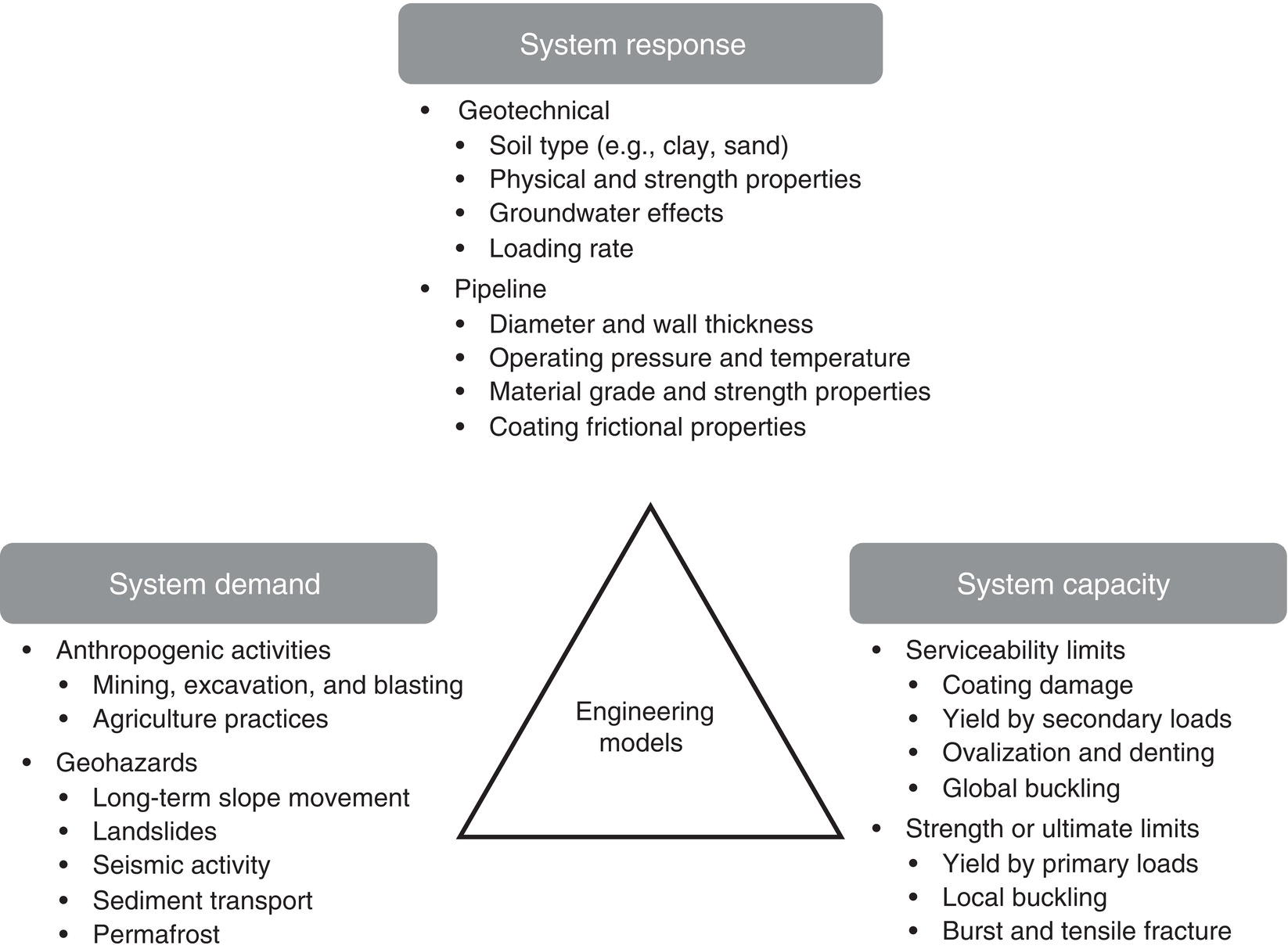
13.2 Site Characterization and Geotechnical Engineering in Relation to Pipeline System Response Analysis
13.2.1 Overview
13.2.2 Pipeline Routing
13.2.3 Geotechnical Investigations
13.3 Pipeline/Soil Interaction Analysis and Design
13.3.1 Overview
13.3.2 Physical Modeling
13.3.3 Computational Engineering Tools
13.3.3.1 Analytical Solutions
13.3.3.2 Structural Pipe/Spring Models for Buried Pipelines
Overview
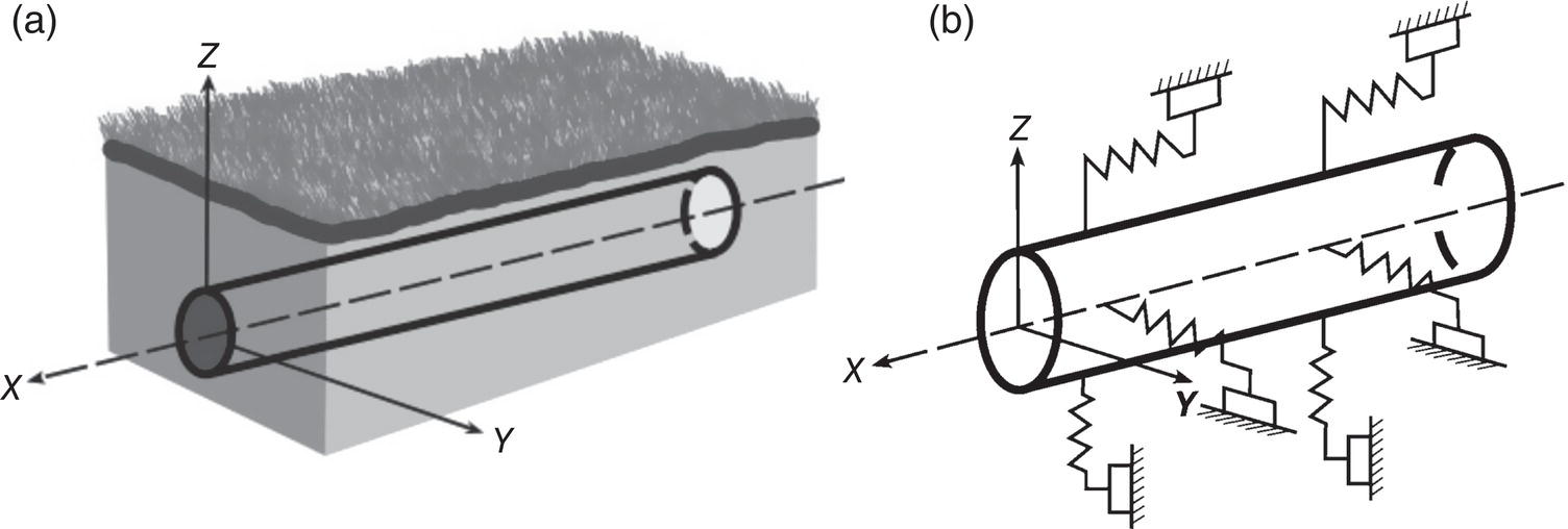
Longitudinal Axial Soil Response

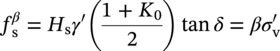


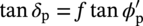
Transverse Lateral Soil Response
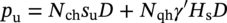
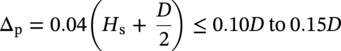
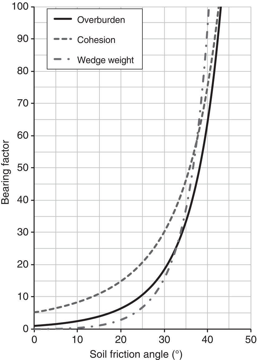
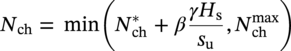
 ) is approximately 11, which is consistent with the lateral loading of piles in cohesive soil [113]. A decrease in the upward movement of the pipeline was also observed with increasing burial depth ratio [195–197].
Transverse Vertical Uplift Soil Response
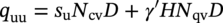
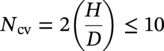
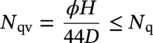
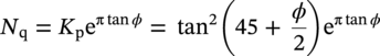


Transverse Vertical Downward Soil Response
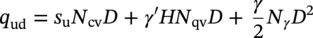
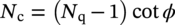
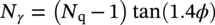
13.3.4 Guidance on Best Practice to Enhance Computational Pipe/Soil Interaction Analysis
13.3.4.1 Overview
13.3.4.2 Structure-Based Models
Overview
Soil Spring Functional Relationship
Influence of Trench Backfill and Native Soil
Interaction Factors
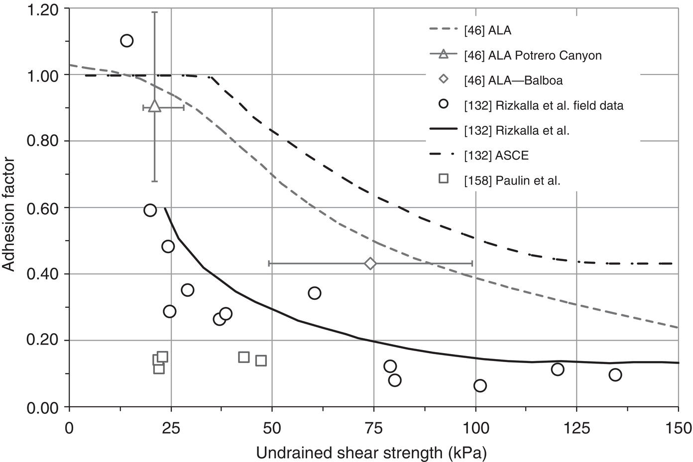
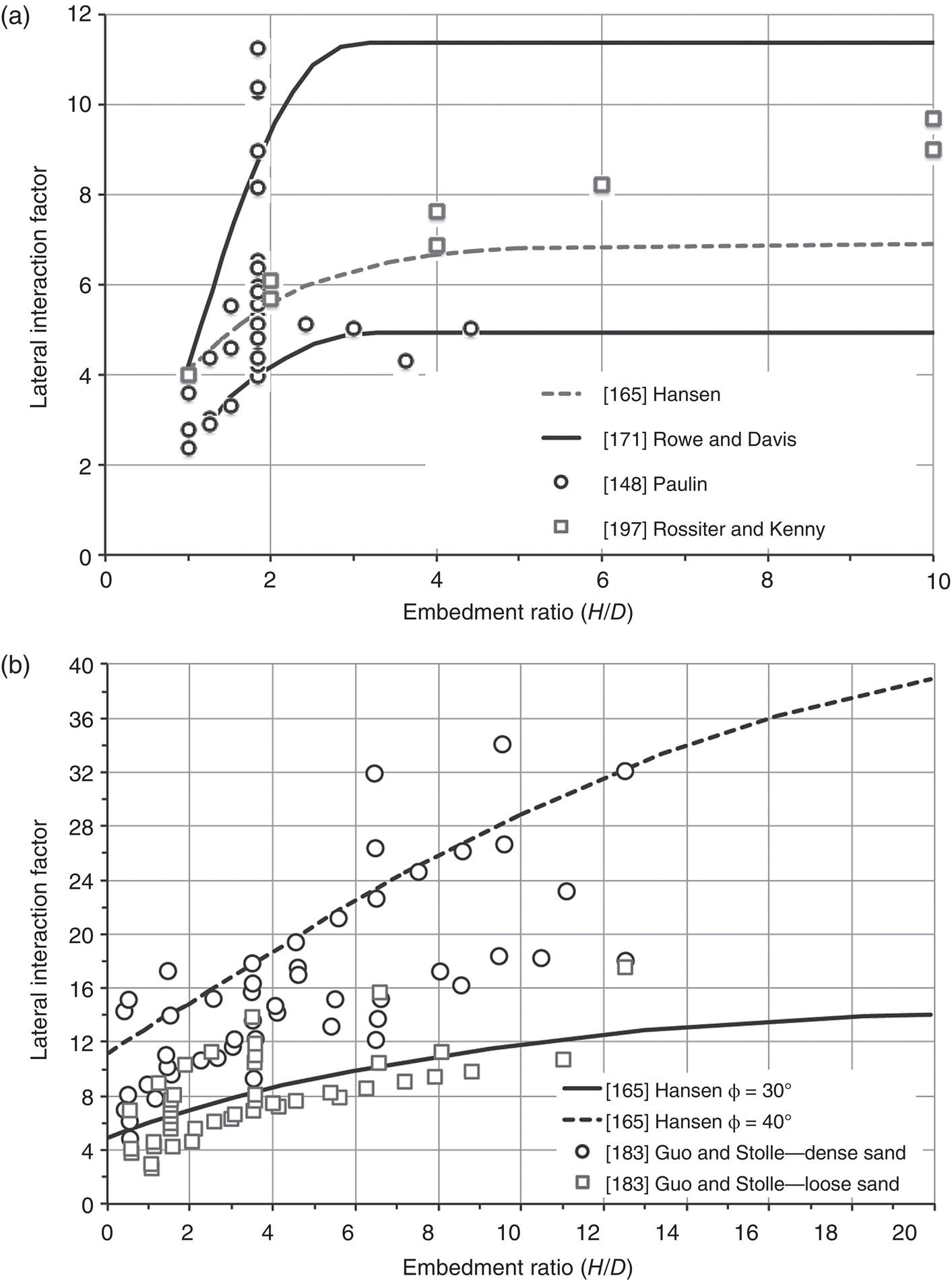
13.3.5 Emerging Research
13.3.5.1 Oblique Loading
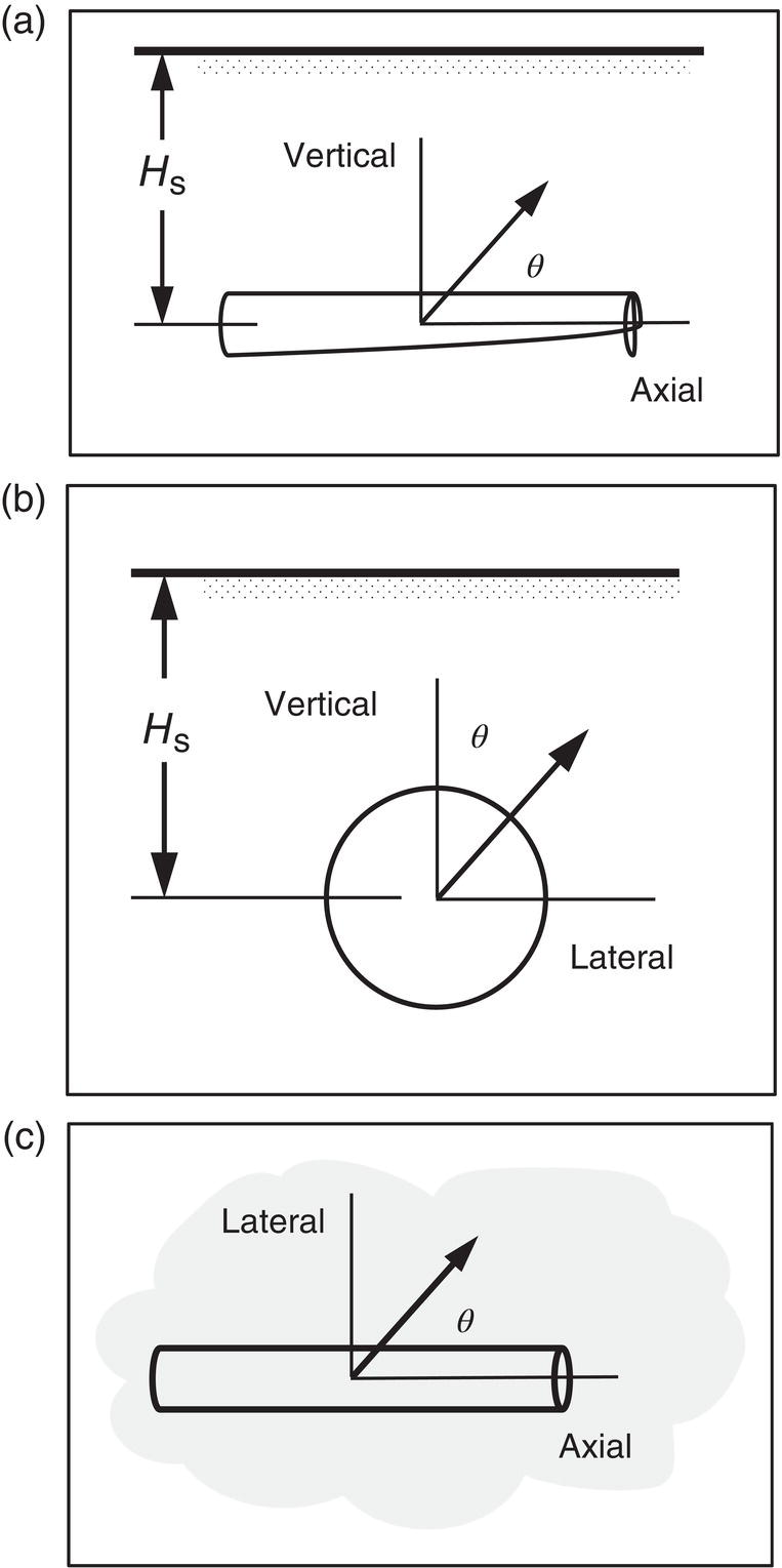
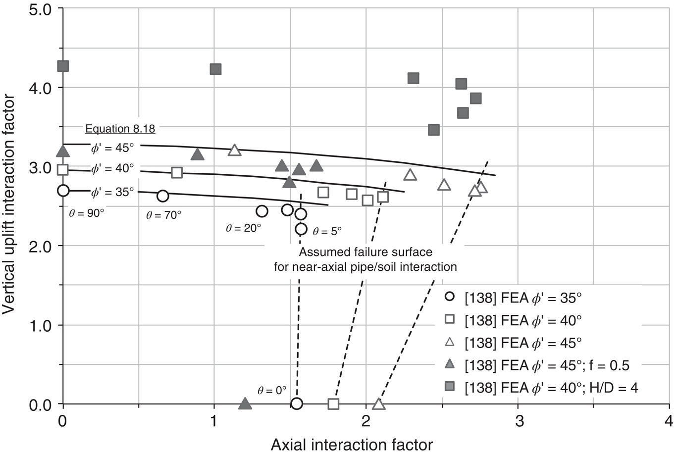
Vertical–Axial Interaction
Vertical–Lateral Interaction
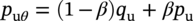
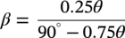
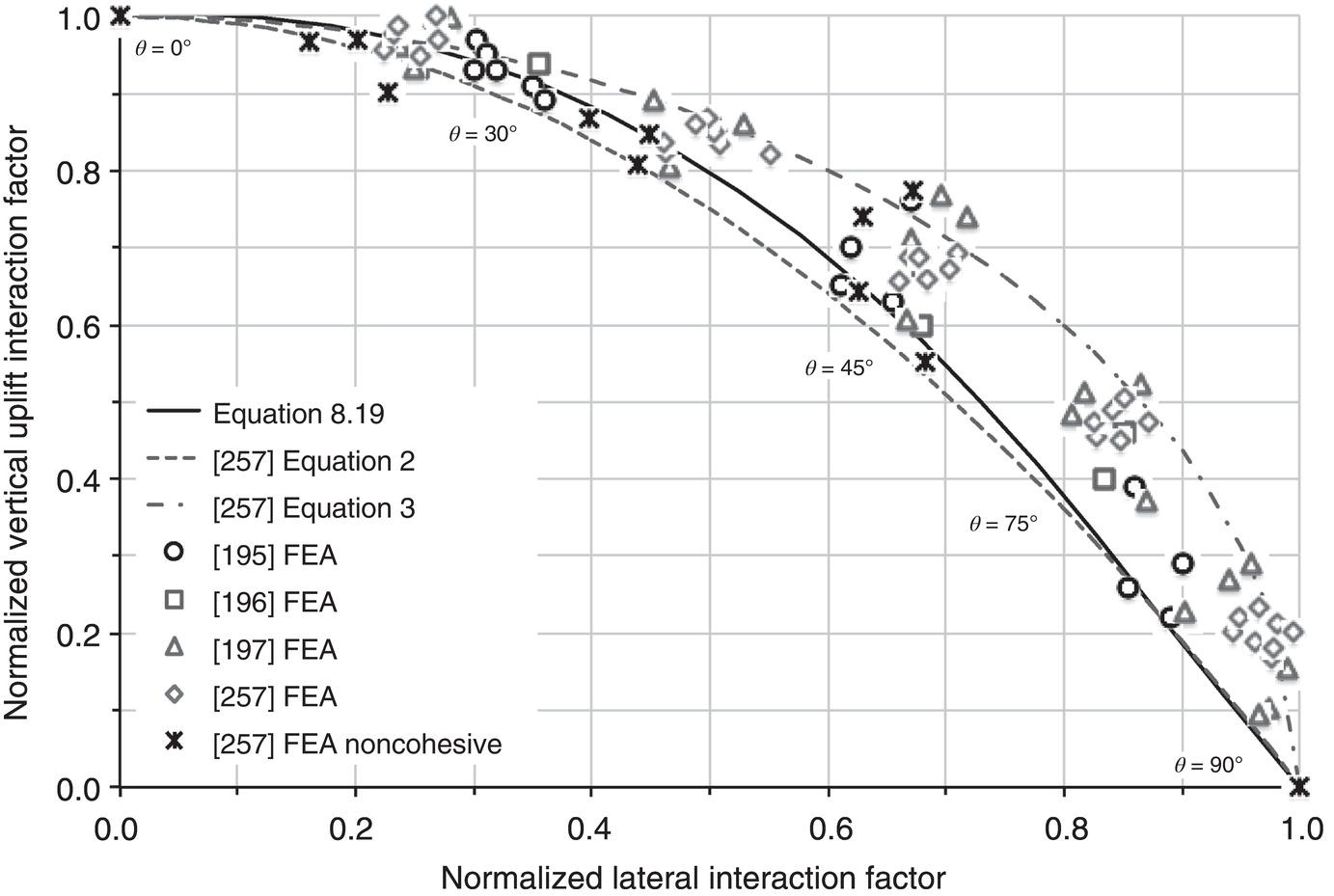
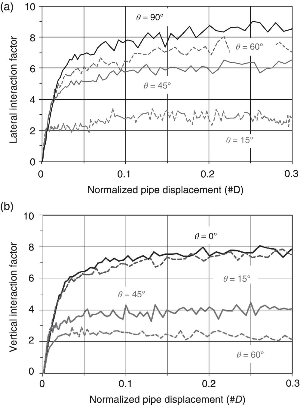


Lateral–Axial Interaction
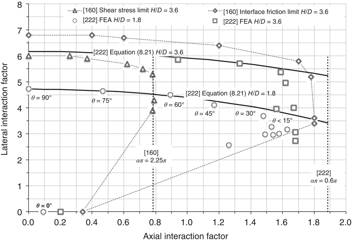

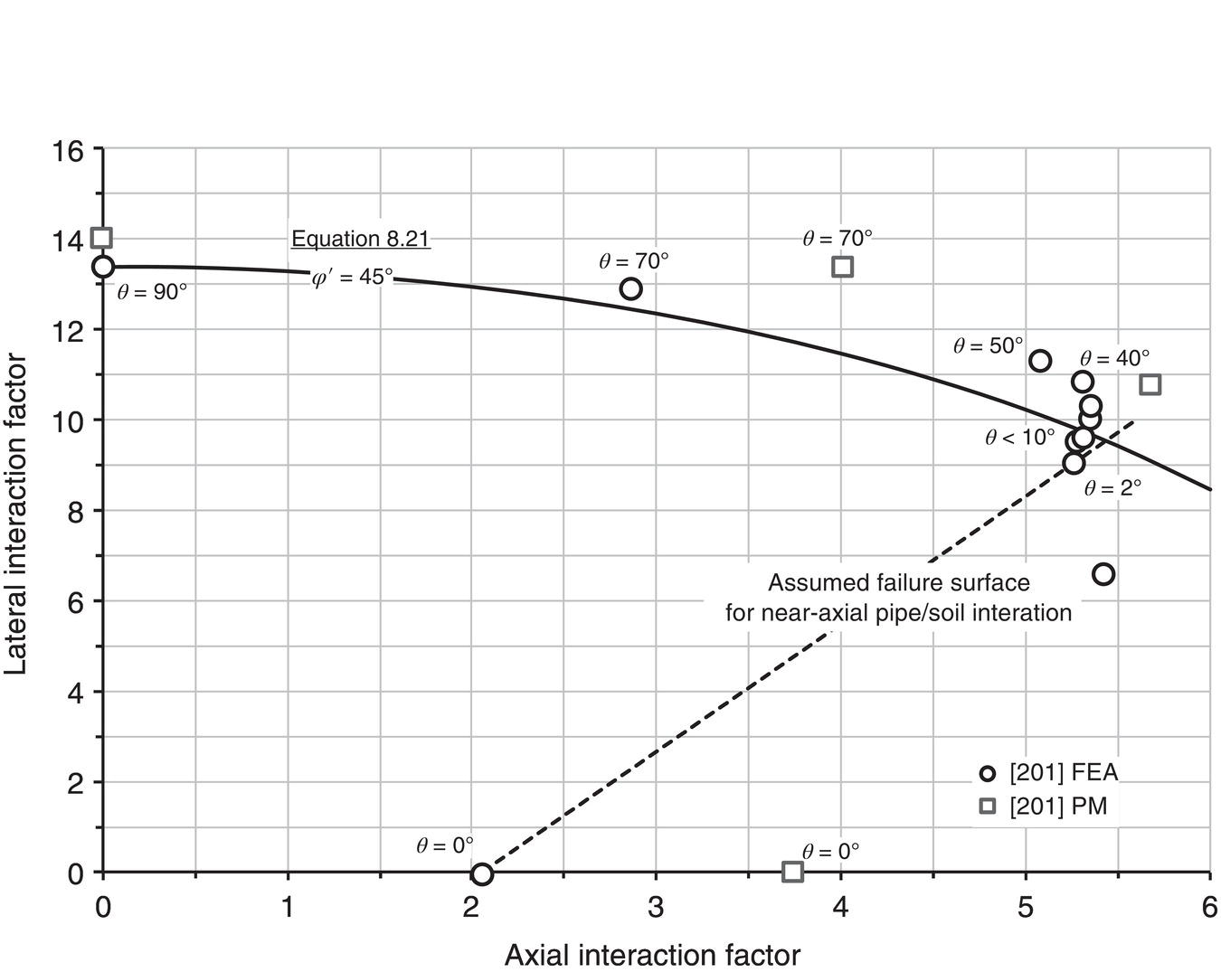

13.3.5.2 Loading Rates
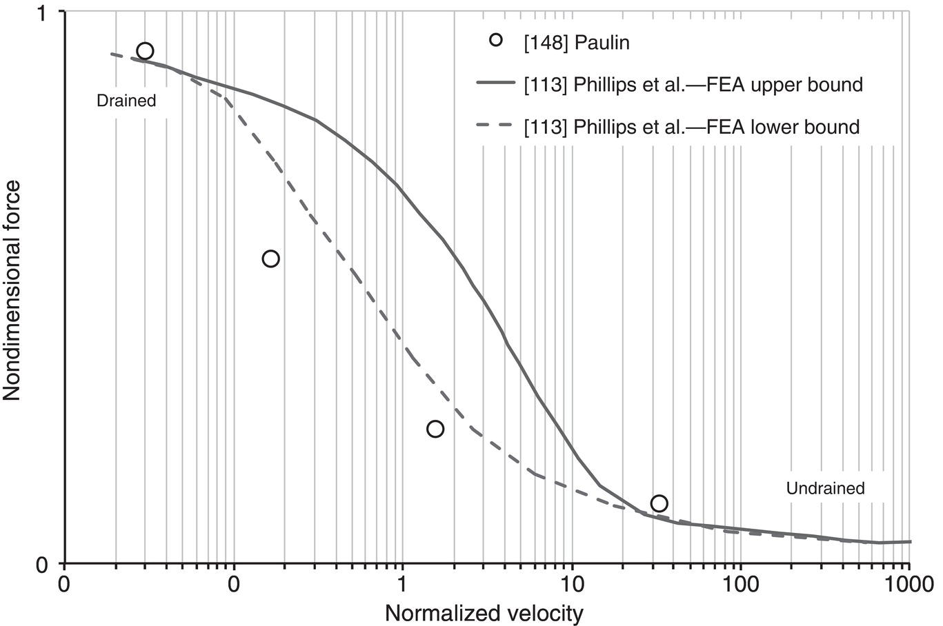
13.3.5.3 Large Deformations: Load Coupling and Superposition
13.3.5.4 Pipe Diameter and Model Scale Effects
13.3.6 Soil Constitutive Models
13.3.6.1 Overview
13.3.6.2 Elastic Parameters
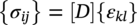
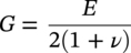
 ) with volumetric strain (εV),
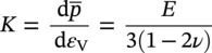
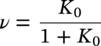
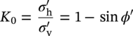


 ) and deviatoric stress (σij):
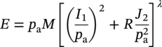
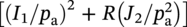 , the modulus parameter, M, and exponent, λ, can be derived. The slope represents the exponent, λ, and the stress invariant modulus, M, can be determined as the value of (E/pa) at
 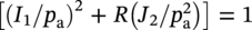 . Typical values for the stress invariant modulus, M, range from 400 to 1200 and exponent, λ, from 0.2 to 0.4 [331].
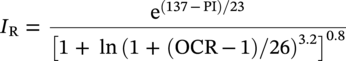


13.3.6.3 Plasticity Models
Overview
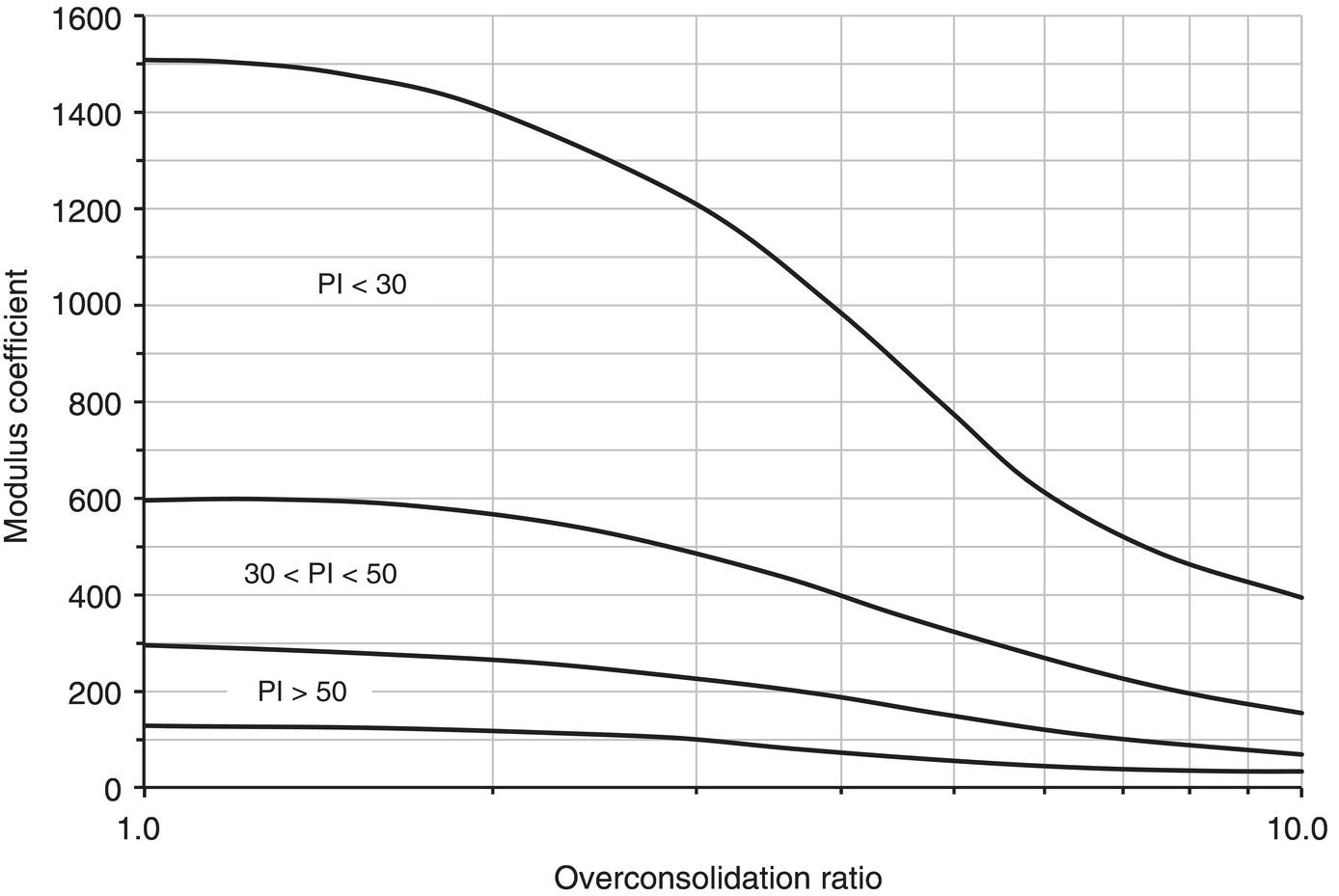

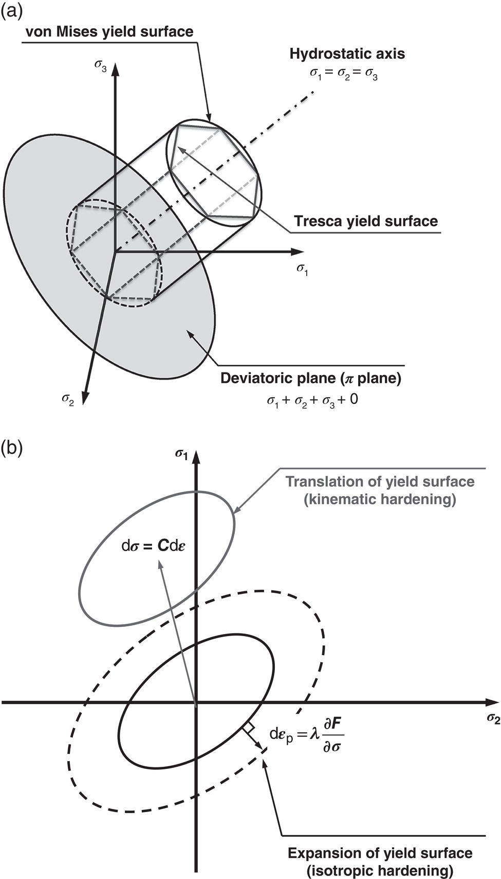
Classical Plasticity Models

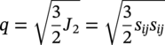

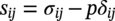

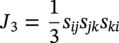
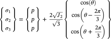
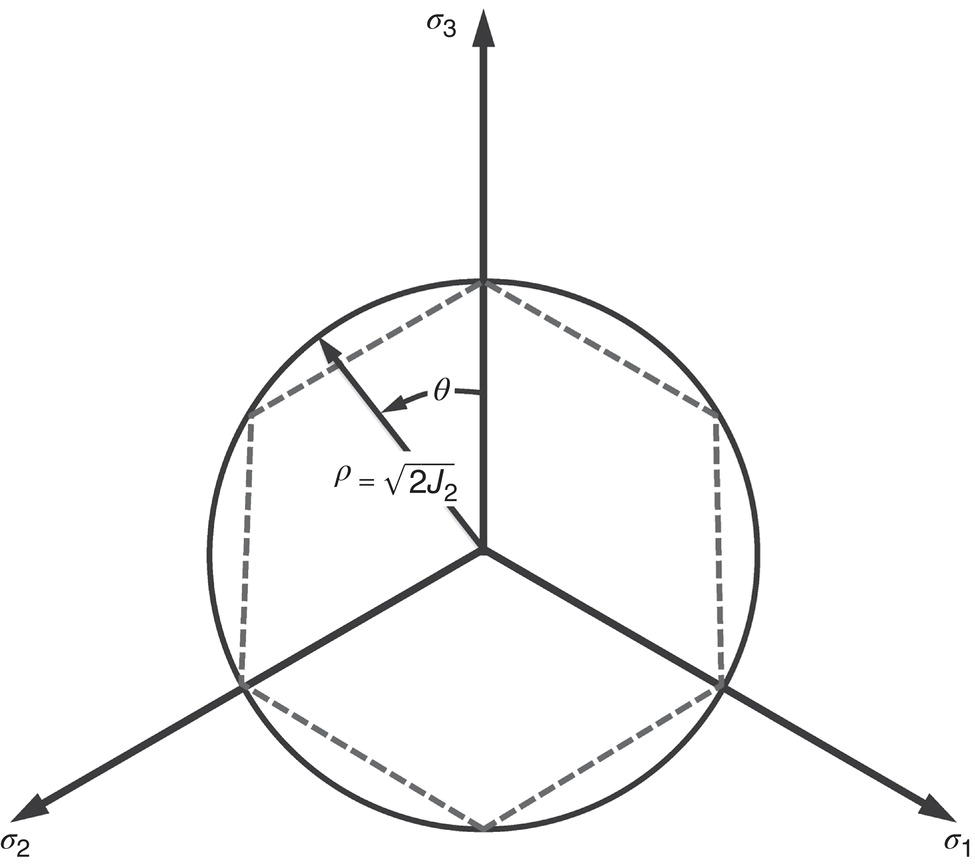
 defines the von Mises yield surface, whereas the Tresca yield surface is represented by a regular hexagon (Figure 13.19).


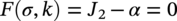

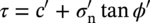
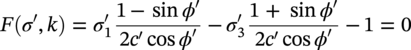

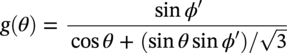
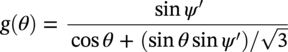

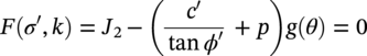

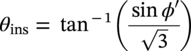
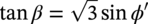
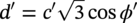
Advancement of Classical Plasticity Models for Application in Soil Mechanics
13.3.6.4 Critical State Models
13.3.7 Advancing the State of the Art into Engineering Practice through an Integrated Technology Framework
Nomenclature
D
outside pipe diameter (m)
E
elastic modulus (MPa)
f
interface friction factor accounting for the pipe coating material at the pipe/soil interface

skin friction per unit area based on total stress (kPa)

skin friction per unit area based on effective stress (kPa)
G
shear modulus (MPa)
H s
burial depth to pipe springline (m)
I 1
first stress invariant or effective stress tensor (N/m2)
J 2
second invariant of the deviatoric stress tensor (N/m2)
K
bulk modulus (MPa)
K 0
lateral earth pressure coefficient at rest
K p
passive earth pressure coefficient
M
dimensionless modulus in the Lade–Nelson hypoelastic model
N ch
transverse lateral bearing capacity factor for cohesive soil
N qh
transverse lateral bearing capacity factor for noncohesive soil
P a
atmospheric pressure (kPa)
p u
ultimate transverse lateral soil load per unit pipe segment length (kN/m)
q ud
ultimate transverse vertical downward soil load per unit pipe segment length (kN/m)
q uu
ultimate transverse vertical upward soil load per unit pipe segment length (kN/m)
R
material constant, 6(1 + v)/(1 − 2v) = 9K/G
S u
undrained soil shear strength (kPa)
t u
ultimate axial soil load per unit pipe segment length (kN/m)
x
axial soil displacement (m)
y
lateral soil displacement (m)
z
vertical upward and downward soil displacement (m)
α
adhesion factor
δ
pipe/soil interface friction angle, δ = f ϕ′(°)
ϕ′
effective internal friction angle of the soil (°)
γ d
dry unit weight of the soil (kN/m3)
γ′
effective unit weight of the soil (kN/m3)
λ
dimensionless exponent in the Lade–Nelson hypoelastic model
v
Poisson’s ratio
Acknowledgments
References
Pipeline/Soil Interaction Modeling in Support of Pipeline Engineering Design and Integrity
(13.1)
(13.2)
(13.3)
(13.4)
(13.5)
(13.6)
(13.7)
(13.8)
(13.9)
(13.10)
(13.11)
(13.12)
(13.13)
(13.14)
(13.15)
(13.16)
(13.17)
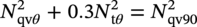
(13.19)
(13.20)

(13.22)
(13.23)
(13.24)
(13.25)
(13.26)
(13.27)
(13.28)
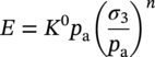
(13.30)
(13.31)
(13.32)
(13.33)
(13.34)
(13.35)
(13.36)
(13.37)
(13.38)
(13.39)
(13.40)
(13.41)
(13.42)
(13.43)
(13.44)
(13.45)
(13.46)
(13.47)
(13.48)
(13.49)
(13.50)
(13.51)
(13.52)
(13.53)
(13.54)
(13.55)