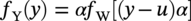
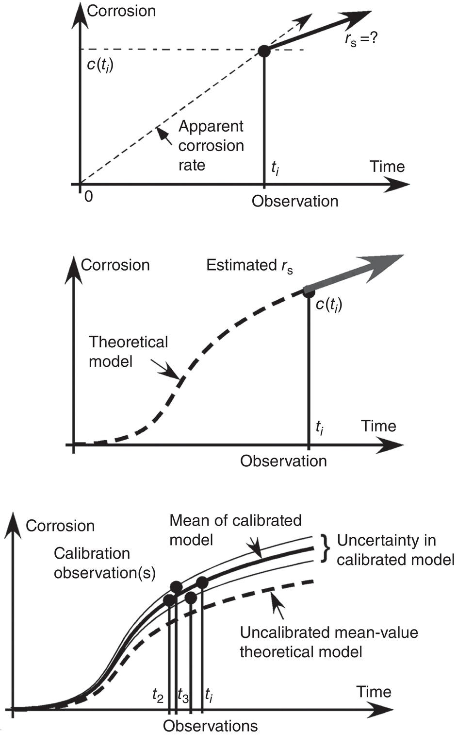
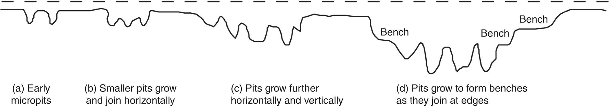
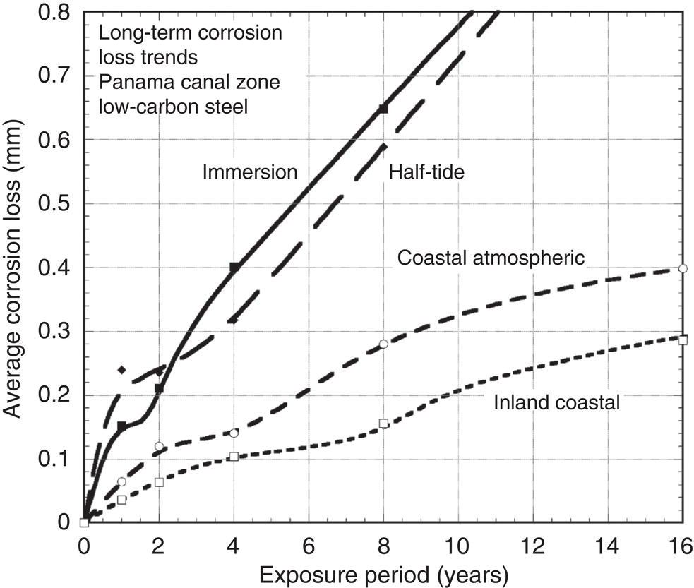
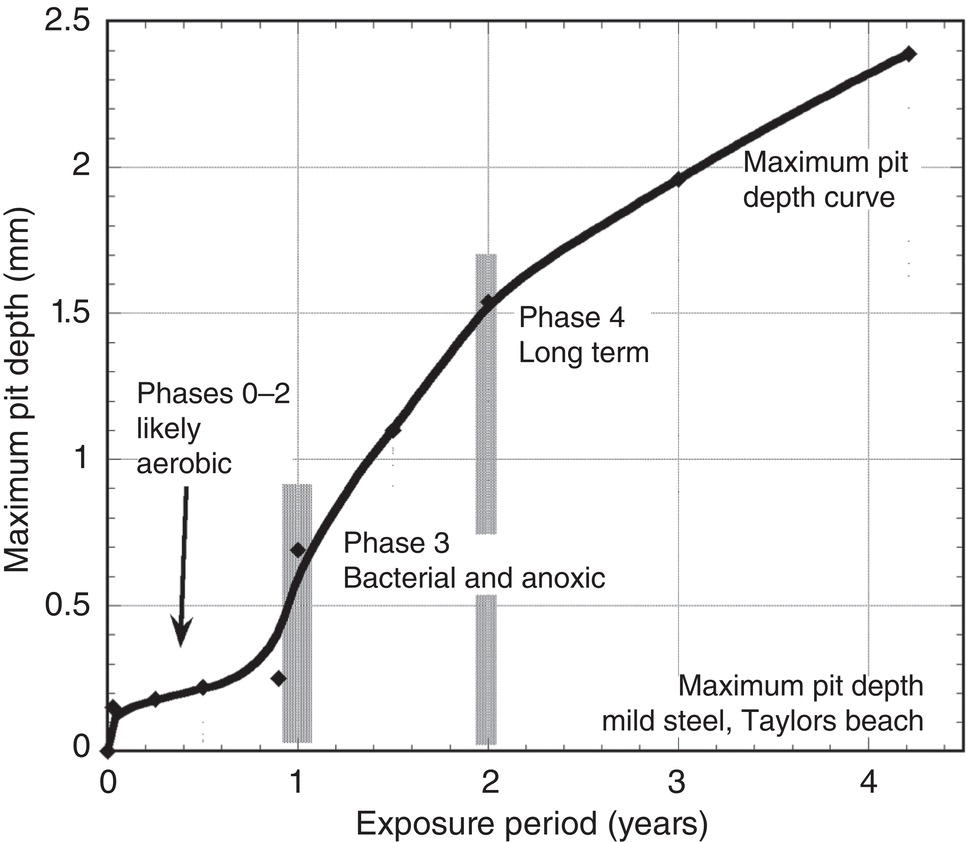
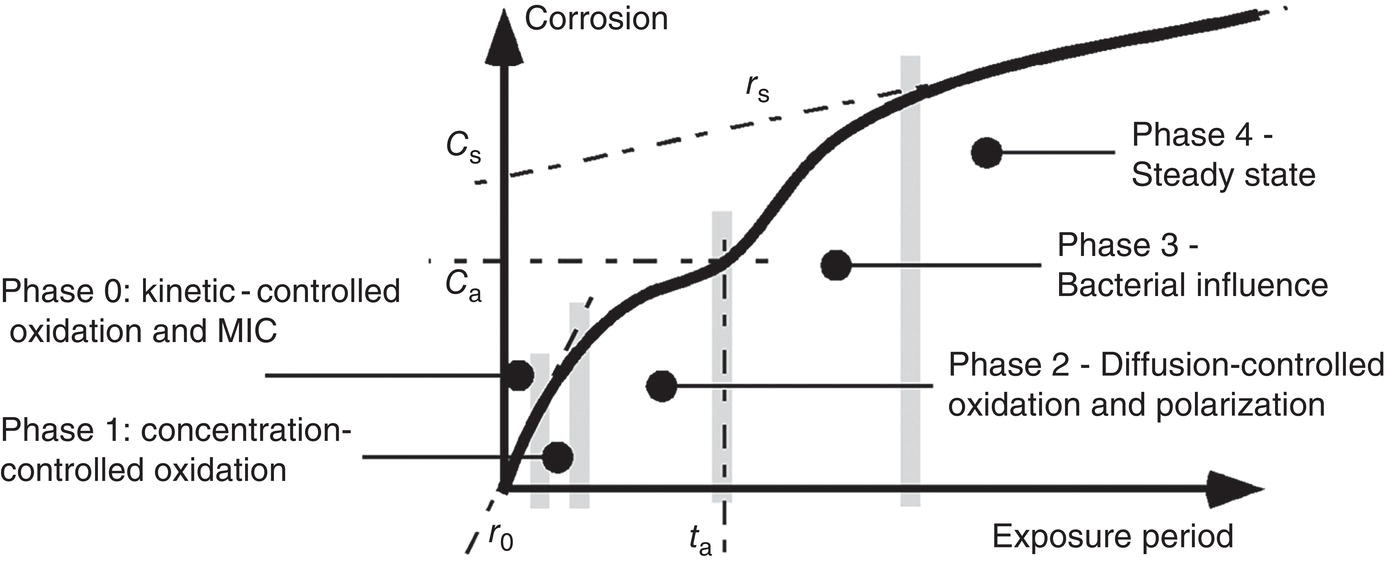
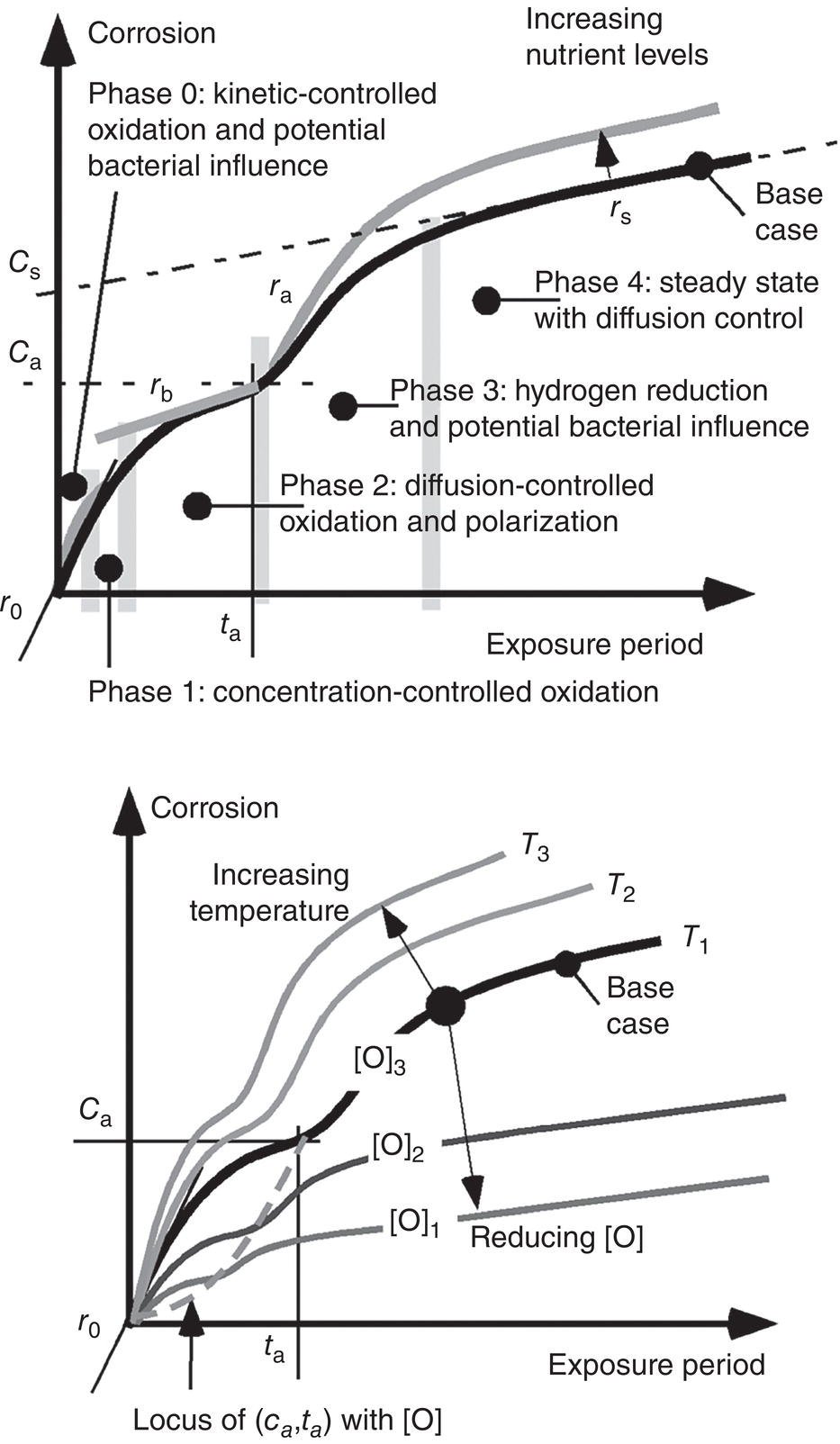
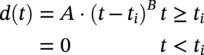
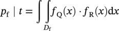
Robert E. Melchers Centre for Infrastructure Performance and Reliability, The University of Newcastle, Newcastle, New South Wales, Australia Pitting is an important form of corrosion that is often responsible for the perforation of physical infrastructure such as pipelines, tanks, and vessels. It may occur for various metal construction materials and for various exposure conditions. In this chapter, discussion is limited to structural and low-alloy steels such as those commonly employed in the offshore oil industry, for ships and for coastal infrastructure. It is also limited to pipelines and so on, exposed to sea and other waters. Generally, such exposure produces rather aggressive corrosion, including pitting. Herein, the development of analytical models to represent the progression of pit depth with increased exposure time and as a function of influencing factors is outlined. Such models obviously must be of sufficient simplicity to be used in practice. The development is built on a very brief review of the extensive literature and research on nucleation, initiation, and early growth of pits, although for infrastructure applications, these early phenomena are of lesser interest. The model for the progression of pitting corrosion described herein is based on reasonable assumptions from corrosion science and is also based on field observations. There is only very limited discussion of this topic in the corrosion science or engineering literature. A summary is given of the principal factors known to influence pitting corrosion, including steel composition and water quality. Since the risk associated with corrosion, and in particular, the risk associated with pitting and perforation, such as for pipe or vessel walls, is of interest in most practical applications, a short overview is also given of relevant theory and techniques for the assessment of structural reliability. This sets the scene for an examination of the uncertainty associated with maximum pit depth and the application of extreme value (EV) distributions, a tool used for over 50 years for this purpose, but as will be seen, open to new interpretations when examined in the light of better understanding of the development of pit depth with increased exposure time. To complete this chapter, short descriptions are given of some research efforts to estimate the external corrosion and pitting of steel pipelines, and its extension to the external corrosion of welds in marine immersion conditions. Also, a brief discussion is given of the important problem of the internal corrosion of steel pipelines used for water injection systems, noting that this also may have relevance to the severe corrosion sometime observed in oil pipelines. However, the corrosion of oil production pipelines is not considered specifically. Typically, such pipelines are subject to carbon dioxide (CO2) corrosion. By comparison, this is typically much less aggressive except where water (usually present in recovered oil) is present. In this case, the most severe (and often very aggressive) corrosion occurs at the bottom of (near) horizontal pipelines and is attributed to water separation to the bottom of the pipe [1]. It follows that for these pipelines too, pitting in seawater conditions is of interest. While in principle, protective coatings and cathodic protection should provide adequate protection against corrosion, in practice this is not always the case or cannot be applied. There are many cases in practice of older steel infrastructure near or in seawater showing signs of corrosion, despite protective coatings or cathodic protection. Where wear or erosion also is involved, such as for coal or iron ore bulk cargoes for ships, protective coatings last only a very short time and cathodic protection is ineffective. Similarly, for mooring chains in the offshore industry [2] and for water injection pipelines (WIP) [3], protective coatings generally are not effective and cathodic protection has been found to be problematic. This chapter is a revision of Chapter 23 in the first edition of this Handbook. The principal changes are that our researches into practical corrosion and pitting of mild and low-alloy steels have shown that for these materials at least (and also for aluminum) pit depth development occurs somewhat differently in the early stages of corrosion compared to later. Of course for reliability analysis, only the longer term behavior is of interest, even though pitting corrosion studies overwhelmingly have used electrochemical investigations and shorter term (a few years) of field exposures. Focusing on longer term pit development shows that the deeper pitting can be interpreted as consistent with the Gumbel Extreme Value (EV) distribution. It also shows that what might appear as “scatter” in the pit depth data can be related to basic corrosion mechanism for pitting—namely that pit depth develops in steps rather than continuously as usually (implicitly) assumed. Both observations have implications for estimating long-term structural reliability. Asset managers and engineers often are faced with the need to make decisions about the technical adequacy or safety as well as the possible future performance and safety of such infrastructure [4]. Predicting the future rate of progression of corrosion, and particularly, possible future pitting corrosion is of interest. As argued elsewhere, the most appropriate approach for predicting future pitting corrosion is through the development of rational, mathematical, and probabilistic models calibrated to real-world data and observations [5]. As noted, these models should aim to represent the pitting process at a level suitable for engineering and managerial asset management decisions and to reflect the effect of time and other influencing factors. It may be helpful to review, briefly, why models for the progression of pit depth with time are useful for prediction of future corrosion, and also, why they are useful for interpreting observations. The basic ideas are illustrated in Figure 56.1 [6]. Consider first the case in which it is desired to estimate the longer-term rate of corrosion or pitting shown by rs in Figure 56.1a when all that is available is an observation of corrosion c(ti) (or pit depth d(ti)) at time t. The usual approach is to estimate the rate of future corrosion by c(ti)/ti shown as the “apparent” corrosion rate in Figure 56.1a. However, a better estimate of the long-term corrosion rate, given by rs (and also its intercept cs at t = 0), can be obtained if the theoretical model is known, as shown in Figure 56.1b. Note that the model, particularly if properly calibrated to actual field data obtained in past experiments or from field experience, strengthens the prediction since it also brings to bear information and knowledge contained in the model. In turn, this means that the best models are those based both on theoretical concepts and accumulated past experience. Such models differ in concept and in predictive capability from models based only on data. In addition, if multiple observations are available, it is also possible to make estimates of uncertainty or variability in corrosion losses or maximum pit depth, as shown schematically in Figure 56.1c. Such estimates are important for constructing the high-quality models necessary for modern whole-of-life asset decision-making processes [4]. As argued previously [5], the development of such models requires a combination of scientific understanding of corrosion processes and sound approaches to mathematical modeling. Figure 56.1 Corrosion loss observation c(ti) at time ti and the estimated apparent corrosion rate compared with the better estimate rs, estimate of rs based on a known theoretical model, and showing variability estimated from multiple observations. Differences of opinion arise sometimes about the use of the term “pitting.” Some electrochemists would prefer to reserve the term for the highly localized corrosion seen only on metals that have passive films, such as stainless steels and aluminum, and therefore, should not be applied to mild- and low-alloy steels. In this view, the existence of a passive film is a necessary condition for pitting [7]. Herein, the more classical view is adopted, namely, that the term also can be applied to metals without passive films, or weak films, including mild and low-alloy steels. This is entirely consistent with major corrosion researchers and authors such as Evans [8], Butler et al. [9], Uhlig and Revie [10], Szklarska-Smialowska [11], Sharland and Tasker [12], Shrier [13], and Mercer and Lumbard [14], all of whom use the term pitting in relation to mild and low-alloy steels. Although electrochemistry lies at the heart of corrosion processes, much of the discussion to follow in this chapter deals with engineering application aspects and for that purpose, detailed discussion of electrochemistry usually is not necessary, in a similar way that atomic particle physics is not necessary for the understanding of the behavior of a steel bridge. However, to set the scene for an understanding of pitting corrosion, a little background is required. Corrosion may be considered the (electrochemical) transfer of material (steel) away from the original location to somewhere else—usually deposited elsewhere as oxidized iron (i.e., rusts) but also lost into the surrounding environment (usually water or moisture). This process is accompanied by the physical transport of electrons (i.e., energy) released from the sites where metal is lost (the anodes) to those sites (the cathodes) where metal is deposited and oxidized, usually by oxygen (although other electron acceptors may be involved). In contrast, in purely chemical reactions, there is no distinction between anodic and cathodic sites and the electrons involved in the reactions simply move from one electron orbit to another [15]. Typically, there are numerous anodic and cathodic sites on a surface subject to corrosion and these may be very close to each other (nanometers) or much further apart, provided there is electrical conductivity between them. In active corrosion, the conductive paths must include both the steel and water (or other electrolyte) in series. The driving force (electrical potential) for the corrosion current is the result of very small differences in the surface topography and grain structure of a steel surface. This results in very small (electrical) potential differences. These provide the initial driving force for electron flow. For metals such as stainless steel and aluminum, which have a so-called passive film, this stage is also known as pit “nucleation” in the pitting corrosion literature [7, 16]. Mild steel does not have a significant passive film and the process is slightly different, which, for passive films, has received by far the most attention in the corrosion science literature [17]. However, an important mechanism for pitting, including for mild steel, is the likely involvement of sulfide (and other) inclusions that are almost invariably present in all commercial steels [18], something recognized many years ago [19–21]. In both cases, the overall effect is much the same—the surface corrodes at localized (anodic) areas under overall readily available oxygen conditions, with the corrosion products (the oxidized metal) forming mainly at and near the cathodic regions. The process is driven by differences in localized electrical potential and produces localized corrosion at a microscale. On the other hand, in metals with passive films, there usually is some delay before the passive film is ruptured and pitting commences, pitting for mild and structural steels commences almost immediately, as demonstrated by careful experimental work [9]. In theory, the rate of corrosion, and thus, also of pitting, can be expressed through the rate of flow of electrons either over larger areas (as for general corrosion) or on small areas (as for pitting). As in any electrical circuit, the rate of electron flow that will occur (and thus, the theoretical corrosion rate kinetics) depends on the resistivity of the path (steel) through which electron flow (or current) occurs. This mechanism is employed for electrochemical measurement in some types of laboratory experiments [16] and then used sometimes to explain the rate of corrosion under particular circumstances. However, for most practical situations, this is largely theoretical. In practice, most corrosion processes in wet environments are rate controlled by the rate at which the critical diffusion process can occur. Candidate diffusion processes include the diffusion of ferrous irons out of the localized corrosion regions and later out of the pits and also the diffusion of oxygen from the external environment toward the cathodic sites. In actual corrosion pitting, one of the diffusion processes usually is the rate-limiting step, controlling the rate of corrosion, since typically the diffusion processes are much slower than the kinetic reactions (electron or corrosion current flows) [16]. As will be seen, this distinction is crucial in modeling the corrosion process under realistic conditions. Figure 56.2 Development of pitting as a function of time, showing initial pitting broadening out to form a plateau on which new pits then form. ([23]/with permission of Elsevier.) Figure 56.3 Successive views (a, b, c) of pitted surface of steel coupons. (Height of images approximately 1 mm). ([23]/with permission of Elsevier.) Actual observations of the progression of corrosion of mild or structural steels in seawater support these concepts. Usually, already within hours of first exposure, very small areas of localized corrosion or pits can be seen to have developed on a steel surface. These localized regions grow quickly in depth, reaching perhaps up to some 100 μm [9], within days–weeks of exposure and then tend to stop growing in depth but become wider with further exposure [22]. It has also been observed that many early pits stop growing soon after formation and are “overtaken” by others [11]. Figure 56.2 shows a schematic view of the development of pitting with increased exposure time. In particular, it shows that the initial pits or regions of localized corrosion stop growing in depth but amalgamate to form shallow depressions and that later new pitting develops on the depression surfaces. The result is the formation of a series of depressions and a range of pit depths and sizes. This shows that the growth of pit depth is not a continuous process, at least for longer exposures. Figure 56.3 shows some microscope photographs (at the same scale) of the progression of pitting [23]. This pattern of behavior for pit growth and development contrasts with the conventional wisdom, which assumes a continuous single functional process for pit depth development. Real seawaters are more than “salt water” and typically contain a wide range of chemicals and biological materials. For metals exposed to real seawater invariably, there also will be a colonization of the steel surface by biofilms [24]. These can provide environments suitable for colonization by microorganisms. In turn, these may provide electron acceptors alternative to oxygen, and thus, contribute to the corrosion process. There is a wealth of laboratory observations of the contribution of microbiologically influenced corrosion (MIC) to initial and short-term corrosion losses and to early pitting [24]. Usually, these experiments are conducted in solutions with artificially high levels of bacterial culture and high supplies of nutrients necessary for microorganism metabolism [25]. There is evidence also in field exposure conditions of increased mass losses for waters with elevated levels of nutrients, for both short-term [26, 27] and long-term exposures [28], including in brackish and fresh waters [29, 30]. In addition, more recent controlled experimental observations of steel surfaces exposed to normal coastal seawater show that the presence of microorganisms has a strong effect on localized corrosion and pitting when compared with the surfaces resulting from corrosion in essentially sterile seawater and that this effect continues for many years [31]. It follows that microbiological factors can have an important influence on the severity of pitting corrosion. Although Figures 56.2 and 56.3 show the development of pitting under seawater exposure conditions, it is important to note that similar observations have been made in laboratory experiments using triply distilled water and at elevated water temperatures (70 °C) [14]. This means that this type of corrosion behavior is not confined just to seawater exposures and is not necessarily related to the effect of microorganisms, although as discussed earlier, they can be involved [32]. It now should be clear that the corrosion of a steel surface in various waters, including seawater, is a complex, changing phenomenon. This means that any microscopic examination of a corroded steel surface will reveal only a “snapshot” of a complex mix of larger and smaller pits as well as regions that may not yet be unaffected by corrosion. It also shows that so-called uniform or general corrosion, widely used in corrosion studies, is actually an idealization of a more complex situation. However, in practical applications, it is still a convenient concept and is readily ascertained from changes in mass loss of nominally identical coupons exposed for different periods of time. This is much easier to measure than pit depths or the form of an undulated surface consisting of pits and depressions (e.g., Figure 56.3). Examples of corrosion mass losses as functions of exposure period are shown in Figure 56.4, for four different marine exposure environments, including tidal and atmospheric exposures [33, 34]. Similar trends have been interpreted from published data for many other exposure sites [35]. Maximum pit depths for the sites shown in Figure 56.4 have been reported. However, the data trends are inconsistent, sometimes showing pit depths at some exposure periods being (much) lower than what was observed for the preceding period. This cannot be true in actual exposure conditions but is the result of the experimental difficulty of measuring actual (absolute) pit depths relative to the original surface. Usually, all that can be done is to measure the pit depth relative to some part of the remaining surface and then to add an allowance, based on mass loss to estimate the absolute pit depth. This attempts to allow for the plateaus shown in Figure 56.2. For maximum pit depth, Figure 56.5 shows the measurements of pit depths corrected to produce estimates of absolute pit depth for mild steel exposed to coastal seawater for up to 4 years. Figure 56.4 Corrosion as measured by mass loss for different exposure zones in the Panama Canal Zone, based on reported data with trends curves added. Figure 56.5 Typical growth of pit depth with increased exposure time as inferred from observations of mild steel coupons exposed to coastal seawater. (Adapted from [36].) It is seen that pits develop very soon after first exposure to a maximum pit depth that then changes little for some time (about 8 months in Figure 56.5) after which there is a gradual increase followed by a very considerable increase in pit depth and this continues, at a gradually reducing rate, for several years. Overall, the pattern (but not the relative intensities) is similar to the trends shown in Figure 56.4 for “general” corrosion. However, it will be seen that the increase in the rate of corrosion after time ta is much greater than that for mass losses shown in Figure 56.4, reflecting the concentrated corrosion inside pits. Similar trends for maximum pit depth have been observed for many other field trials [36]. Because of the close links between pitting and general corrosion outlined earlier, it is not surprising that Figure 56.5 shows the same general characteristic functional form as seen for general corrosion loss as a function of time (Figure 56.4), although as noted, it is much more severe in phases 3 and 4 for pitting than it is for general corrosion. This functional form can be considered “bimodal.” It forms the basis for the approach to modeling the progression of pitting corrosion with increased exposure time. It also has been found to be useful in explaining various practical observations for corrosion loss and for pit depth. The characteristic functional form for the progression of corrosion and for maximum pit depth shown in Figures 56.4 and 56.5 has been found to occur in many data sets [35, 36] and led directly to postulating the bimodal model shown in Figure 56.6, first developed for mass loss as a function of exposure period. It consists of a number of sequential phases, 0–4, each representing a different corrosion rate-controlling mechanism. Modes 0–2 occur before and modes 3 and 4 after time ta (Figures 56.5 and 56.6). The corrosion rate-controlling mechanisms in phases shown in Figures 56.5 and 56.6 may be summarized as follows. Immediately upon first exposure, the corrosion loss trend consists of a very short phase 0. During this time, corrosion initiates and also, for seawater, the metal surface is colonized by biofilm and then by microorganisms. In phase 1, the rate of corrosion is controlled by the rate of diffusion of oxygen from the water or moisture immediately adjacent to the metal surface (“concentration control”), while in phase 2, the corrosion rate is controlled by the rate of oxygen diffusion through the increasing thickness of corrosion products on the metal surface. This produces the characteristic attenuation of the rate of corrosion. Eventually, at around ta, it becomes possible for anoxic condition to govern the rate of corrosion, through aggressive pitting corrosion under the rust products. This may involve microbiological activity within the rust layers adjacent to the metal surface [37]. This is phase 3. Phase 4 represents a long-term, probably near-steady-state, corrosion condition. The bimodal trend is not confined to the corrosion loss of mild steel in seawater. Without going into detail, the development of the bimodal model for “general corrosion” or corrosion loss and, importantly for pit depth development, has been shown in very detailed experiments [38]. These showed that pitting is an essential process in the development of the bimodal model for corrosion loss and, important for the following discussion, that the corrosion processes change with the phases (0–4) in the model. For pitting, Figure 56.5 shows very clearly that the rate of growth of maximum pit depth in phases 3 and 4 is very much greater than in phase 2 and also that the pits are much deeper than in phase 2, particularly, when compared with the bimodal trend for mass loss (Figure 56.4). As noted, in part, this reflects the fact that the deepest pits occur over relatively small areas of a steel surface and that the electron currents that are essential in the corrosion process are concentrated there. In part, also, it is the result of the mechanisms involved in pitting in phase 3 being much more aggressive than earlier, being the result of an autocatalytic reaction process of steel that can occur under the localized anoxic conditions [18]. Such conditions will exist under the corrosion products and as part of the highly irregular corroded surface formed earlier during corrosion in phase 2. In addition, the highly nonhomogeneous nature of the corroded surface also permits, under the anoxic conditions that will prevail, the activity of obligatory anaerobic bacteria such as the sulfate-reducing bacteria, to flourish during phase 3 and add to the severity of local corrosion [39], provided of course that nutrients are available. Experimental evidence for this mechanism is available [31] and evidence from field trials shows correlation between corrosion and pitting and nutrient concentration in the water [27, 29, 40]. A more detailed description of the reactions and mechanisms involved is available [32]. Mathematical formulations exist for the most important phases shown in Figure 56.6 [35, 41]. Also, the bimodal model has been calibrated to a range of field observations reported in the literature using the results reported for independent field investigations. For example, Figure 56.7 shows the calibrated variation of the model parameter ta with average seawater temperature [35]. Figure 56.6 Bimodal model for marine corrosion loss (and maximum pit depth) as a function of exposure period. Parameter ta defines the transition between the modes. Figure 56.7 Variation of ta with average seawater temperature based on worldwide data. (Adapted from [36].) It is evident that the progression of pit depth d(t) over extended periods of exposure time t does not follow a simple constant “corrosion rate,” implying a linear function. It also does not follow, except perhaps for short exposures, the so-called power law, widely used to represent the progression of corrosion [42] as well as the development of pit depth [43]. Typically, it has the form where d(t) is a characteristic dimension such as pit depth or diameter and ti is the time to pit initiation. A and B are the constants obtained from curve fitting (1) to experimental data. The power law, or the simplified expression d(t) = A.tB, is relevant for relatively short periods of exposure, usually much <1 year and more usually measured only in hours or days. Moreover, the calibrations have been based on laboratory observations [11]. As an approximation, Equation (56.1) can be used to represent the progression of maximum pit depth for phases 0–2, but as shown in Figure 56.5 (and much other data besides), the corrosion mechanisms in these phases are very different from those in phases 3 and 4, as clearly seen in the bimodal characteristic. Representing the whole of the data set such as shown in Figure 56.5 by Equation (56.1) loses the subtleties of the various rate-controlling processes, described in considerable detail in [38]. As will become clear when the statistics of maximum pit depth are considered ahead, this can have considerable ramifications for predicting the likely future maximum pit depths and their uncertainty. Apart from structural size, orientation, steel composition, and grain structure, a considerable number of environmental factors may influence the pitting corrosion of structural (carbon) steels. For example, for seawater corrosion, Table 56.1 summarizes the known effects [44]. Schematic representations of the effect of three of the most important effects, nutrient levels in the water, water temperature, and concentration of dissolved oxygen in the water on corrosion, and hence, on pitting, are shown in Figure 56.8. There is insufficient space for a review, but details of these and other effects have been described in the literature. For pipelines, both structural strength capability and containment are important design and operational conditions. Modern trends are to move away from “factors of safety” and to consider instead risks or reliability [1]. The reliability of pipelines can be presented as a conventional structural reliability problem and represented in the space of both loading and resistance and time t as shown in Figure 56.9. It shows a stochastic loading process system Q(t) and a time-dependent, monotonically decreasing random variable resistance R(t). The joint probability density at any time t of Q(t) and R(t) is denoted fQR(t). Both Q(t) and R(t) can comprise multiple components to represent more complex systems. Of interest is the probability of failure Pf(t) as a function of time t. This is a function of the decreasing nature of the resistance or load capacity R(t) of the system. Table 56.1 Factors Known to Influence Corrosion of Steel in Seawater Figure 56.8 Influence of nutrients to support microbiological activity, average water temperature, and average oxygen concentration on the “base case” bimodal model for corrosion of mild steel in seawater. ([37]/with permission of Elsevier.) Figure 56.9 Schematic relationship between loading process Q(t), deteriorating resistance R(t), and the time-dependent probability of failure pf(t). At any time t, conventional structural systems reliability theory defines the probability of failure as [45] where fQ(t) is the (conditional) probability density function (PDF) for Q and similarly for R at t. The failure domain Df may be defined through a limit state function (or performance function): where X collects all the relevant random and other variables, which, for the simplest case shown here, are simply Q and R. If one or more of the components of X is time dependent, G(X) is also time dependent. Stochastic variables may be included in various ways but often the simplest approach is to consider them using a combination rule such as Turkstra’s [45]. For any structural reliability problem, the crucial matter for definition is the limit state function (or functions) G(X) describing the condition(s) considered to constitute failure of the system. For pressure pipelines supported by soil or within soil or in water, this may include [1, 46] bursting, bending moment and/or shear load limitations, crushing all with or without corrosion of the pipe wall leading to unacceptable leakage, or simply to corrosion of the pipe wall without other influences. Here, only the latter case will be considered. The limit state function for wall perforation through pitting corrosion can be considered the event when the deepest pit is equal to or exceeds the local wall thickness D. In practice, D is likely to be a random variable with spatially varying properties. Ignoring these for the present as second-order effects, the limit state function for the case of the deepest pit first penetrating the wall thickness D can be written as where dmax(t) is the maximum pit depth at time t. It is best treated as a random variable. Its statistical properties are required to determine (56.4) and thus to evaluate (56.2). Since dmax(t) is a maximum over many individual pit depths, EV theory provides an appropriate approach to estimating its statistical properties. In the following, attention is given to determining the statistical properties of dmax(t) since once these are obtained the structural reliability analysis can be carried out. The details of the calculation procedures are well-established [44] and are not considered further herein. If failure of the pipeline can be defined only through the probability of pipe-wall perforation by pitting, without consideration of any possible failure mechanism and without consideration of uncertainties in wall thickness D, a simpler approach can be adopted. In this case, the probability of failure for any time interval t from zero becomes In many applications, the maximum pit depth that may occur at some point in time is of prime interest. There is a long history of assuming that the probability distribution describing the uncertainty in maximum pit depth can be represented by an EV distribution. The theoretically correct EV distribution for the maximum of (independent) values of maxima is the Gumbel distribution for the maxima [47] and this applies to pit depths. Pitting corrosion usually is considered one of the prime applications of EV analysis [47] and has been applied since the early work of Aziz [48]. In some cases, other distributions with long “tails” such as the lognormal, Weibull, Pearson 3 or the generalized extreme value (GEV) distribution has been proposed as appropriate [49]. However, unlike the Gumbel distribution, there is no underlying theoretical basis for these choices—their use is purely empirical. Because they are entirely empirical, their application and use require extensive field data for model calibration and for sensitivity analyses for the parameters involved, in some cases tied to models for internal corrosion [e.g. 50]. There are claims also that the classical distributions (including Gumbel) are too restrictive because they require the underlying distribution to be homogeneous and because they seem unable to deal with the evolution of the pitting process, that is, with a change in the underlying pitting process as pitting progresses [51]. A “bootstrapping” approach with the generalized Lambda distribution was proposed. However, this again requires large data sets and has been demonstrated only for quite limited exposure periods on laboratory samples. Ideally what is required is an approach that has an acceptable degree of theoretical foundation, is consistent with the now known development of pitting corrosion over extended periods of time and thus has capacity for extrapolation and that does not require very large data sets for practical applications (as distinct from scientific understanding). The latter is important because there are rather few data sets available in the open literature for pitting. This is particularly the case for corrosion and pitting of the interior of production pipelines (oil and gas.). A limited amount of data is available for WIP [52]. In the following, the classical Gumbel EV distribution will be used as a basis for discussion and exposition as it is the only distribution with a theoretical basis. As will become evident, recent applications involving large data sets have revealed apparently new characteristics about the pitting process. These are very unlikely to have been revealed by the application of heuristic, empirical approaches. To ascertain whether a set of maximum pit depths is consistent with the Gumbel distribution, it is convenient to use a so-called Gumbel plot. This is a graph of cumulative probability against (in this case) maximum pit depth, with the cumulative probability axis distorted in such a way that data that are truly Gumbel distributed plot as a straight, sloping line. Lines with greater slopes denote a greater variability in the data. (The concept may be compared directly with the so-called normal probability plots.) Figure 56.10 shows an example of a Gumbel plot [53]. In Figure 56.10, the right vertical axis shows the conventional cumulative probability (i.e., the probability that the variable of interest is less than the value on the horizontal axis). The left vertical axis shows the standardized variable w, defined as w = (y − u)α, where y is the maximum pit depth having cumulative distribution function (CDF) FY(y) and PDF FY(y) each defined by Figure 56.10 Gumbel plot with maximum pit depth data at various exposure periods for 18 surfaces mild steel plate coupons continuously immersed in Pacific Ocean seawater. ([53]/with permission of Elsevier.) In the language of EV theory, here, u and α are the “mode” and “slope” of the Gumbel distribution, respectively. They are related to the mean μY and standard deviation σY through μY = u + 1.1396/α and σY = 0.40825π/α. Standard techniques are available to estimate the values of FY(y) for individual pit depths in a data set so as to plot the data set on a Gumbel plot. The data sets for different exposure periods shown on Figure 56.10 were treated using the rank order method [46]. In each case shown in Figure 56.10, a straight line can be fitted through the data sets. This indicates that each data set could be considered consistent with, or representable by, the conventional Gumbel distribution. Also, the slopes of the lines (cf. α in Equations 56.6 and 56.7) increase with longer exposure, indicating greater variability in pit depth with increasing exposure period. In the conventional thinking, once the Gumbel distribution has been fitted to the data, it can be used to estimate probability of exceedance [=1 − ϕ(y)] of a given depth of pit for longer exposures and for greater pit depths, simply by extrapolation of the upper (right hand) end of each Gumbel line [47]. The approach outlined above has a long history [48] and has been applied for relatively shallow pits or, similarly, for relatively short-term exposures. Ultimately, it is based on the assumption that each data set is homogeneous, that is, each data point is an independent sample drawn from the same (statistical) population. Closer examination of the pit depth data plotted in Figure 56.10 shows that they do not fit particularly well to the fitted straight line. This may be dismissed as natural variability in data [54] and indeed this is possible. But the examination of pitting behavior and pit characteristics against the underlying assumptions for EV theory reveals a different and more likely possibility. The phases in the bimodal model (Figures 56.6 and 56.8) imply changes in the nature of pitting process from one phase to the next and in particular between the first and the second modes of the bimodal model, that is, between phases 0–2 and phases 3–4. At the very least, this means that the pit depths generated in the first mode are not from the same statistical population as the pit depths in the second mode. This may be true also for the pit populations generated by each of the phases. Thus, for pit data extending over extended periods of exposure time, that is, with some pit already in phases 3 or 4, there are (at least) two different statistical populations for each data set. EV theory using a particular EV distribution requires all data to come from the one population [47]. EV theory is based on the assumption that each sample observation is an independent statistical event or outcome from the (same) underlying distribution. For pitting, it is very unlikely that the pit depths are statistically independent. This can be expected since the corrosive environment is common to the whole steel surface and the surface itself is largely homogeneous except for microscopic crystal structure and its associated inclusions and defects, with the latter tending to become irrelevant as corrosion proceeds. Data on correlation between pit depths are scarce, and only recently it has been shown that there is indeed a high degree of correlation for pit depth on larger steel plate surfaces [55]. Fortunately, a degree of dependence between events or outcomes can be tolerated in EV analysis. This occurs under the assumption of so-called asymptotic independence, meaning that the maximum depth pits may be assumed independent as the total number of pits increases to a large number [47]. Presumably, this is because the very deepest pits are considered likely to occur in nonadjacent areas. In practice, as noted, the pit depths of most interest are the deepest of the deepest and this implies, for extended periods of exposure, pits in phase 4 (Figure 56.5). Statistical information for the scatter in pit depth values exists from multiple (18 assumed independent) observations of pit depth at each of the exposure periods in Figure 56.5. These data allow the corresponding Gumbel plots to be obtained, one for each exposure period [55]. Figure 56.11 shows the Gumbel plots for pit depth at 3 and 4 year exposures together with the best fit trends and the conventional linear Gumbel trends. It is clear that the latter do not fit very well. Figure 56.11 Gumbel plots for pit depth at 3 and 4 year exposures together with best fit nonlinear trends and Gumbel straight lines. Even though a straight (Gumbel) line could be fitted through each of these data, there is a lot of what could be interpreted as “scatter.” A better approach is to interpret the data differently, in two ways. The first observation arises from the known characteristic of the Gumbel plot that the slope at any point on the plot indicates the scatter in the data, thus, the flatter the slope the higher the scatter [47]. Usually, this is invoked to make statements about the whole of the data set, but it also possible to refer back to the phases shown in Figure 56.5 to identify scatter associated with each of the phases. The net result is shown in Figure 56.12. It shows the (part-) Gumbel trend for each of the phases of the bimodal model. The scatter, or statistical uncertainty, for each pitting corrosion phase corresponds to the schematic probability density functions for the same data [56]. These results should not be unexpected for pit depth data over extended periods of exposure. Unlike short-term tests that may have corrosion and pitting still largely in phases 1 or 2 (Mode 1) and that therefore are essentially homogeneous, pit depth data from extended exposures will consist of a cohort of pits already having some depth, to other pits for which the depth may not be much more than that of newly initiated pits. It follows that for extended exposures the data sets for pit depth are likely to exhibit different trends corresponding to different periods of exposure and thus also for different phases of the bimodal model. This is reflected in the different slopes of the piecewise trends shown in Figure 56.12. Evidently, a degree of judgement is required to fit the best linear (Gumbel) trends through the data for the deepest pits. In particular, it appears that for each of year 3 and year 4, the (independent) pit depth value are greater than expected from a purely Gumbel extrapolation. One possibility is that these are pits generated by imperfect surface cleaning (local under-deposit corrosion), or unusual inclusions or, more likely, an artifice resulting from the way the cumulative probabilities are assigned and then reflected on the probability axis [57]. The latter corresponds with similar phenomena for cases with hundreds of data points (see below). Figure 56.12 Piecewise interpretation of data with each piecewise trend corresponding to a phase in the bimodal model. The second observation from Figure 56.11 is the persistence of “wobbles” in the data trends. Again, these are not isolated phenomena—similar “wobbles” have been observed in pit depth data for long-term exposures [58], and also of cast iron pipes buried (imperfectly) in soils [59, 60] and also for aluminum [61]. In the case of the data in shown Figure 56.11, the “wobbles” can be considered to show a degree of repeatability, with pit depth increments in phase 4 of about 0.38 mm [58], for both 3 and 4 years of exposure (Figure 56.13). The interpretation of these observations is that pitting in practical situations occurs in incremental steps [23]. Indeed, for larger steel surfaces, this can be deduced readily from closely spaced (in time) observations of corroding surfaces of steels [38] and also can be seen in the sequence shown in Figure 56.2. It is consistent with theoretical arguments that once pits have reached sufficient depth they also grow sideways, even in mild steel and similar ferrous alloys [12]. For closely spaced pits (cf. Figure 56.3b) as typical for the corrosion of mild and low-alloy steels, pits may conjoin and leave “plateaus” on which new pitting can initiate, consistent with detailed empirical observations [23, 38]. Figure 56.13 Data as shown in Figure 56.11 for 3 and 4 years of exposure interpreted in each case as consisting of a succession of incremental steps in pit depth. It should be clear from the above analyses that the gross use of all pit depth data for extrapolation to longer periods of exposure or to small probabilities of failure (i.e., higher values of the Gumbel variate w) (cf. Figures 56.11–56.13) would be misleading and usually predict greater probabilities of a given value of pit depth being exceeded (i.e., higher along the right-hand axis of Figures 56.11–56.14). A more accurate approach recognizes that pit depth development follows a bimodal trend overall (Figure 56.12) but that only the long-term trend (phase 4, Figure 56.5) is relevant for reliability assessments. Moreover, within that trend strictly only the deepest pits are of interest—those at the peaks of each of the pit depth increments in Figure 56.13, rather than the average trend as shown in Figure 56.12. This indicates the importance of recognizing that pit depth development occurs in steps, and that this basic behavior is responsible for what appears, at first sight, to be simply randomness in pit depth. Much of the above has focused on one of the primary causes of concern for pipeline reliability—namely, the probability of pipe wall perforation, fostered by the environment within the pipeline or by the external environment. For the latter, protective coating and possibly the effect of impressed current cathodic protection or sacrificial anode protection will need to be considered. Since most pipelines are not protected internally, wet internal corrosion often is the major practical concern. Noting that both crude oil and gas have a water cut, it follows that for these cases and for WIP, the principles for the development of pitting corrosion outlined above are directly relevant for estimating the probability of pipe-wall perforation. In some cases, the external protection of the pipeline may be subject to damage. If the steel is exposed, or left with much less protection eventually localized corrosion of the external steel may occur. Largely because of a lack of detailed knowledge of the extent and severity of such damage and difficulties in analytical or numerical simulation of it for many years, the offshore oil and gas pipeline industry has taken a rather simple but conservative approach to estimating the probability of failure, such as the B31G criterion [62]. Many other simplified analysis methods for reliability estimation of localized corrosion have been proposed, but these were seldom based on actual observations of the way the localized corrosion occurs for actual pipelines. The few field observations that are available have shown that corrosion tends to occur in highly localized areas and to consist of deeper pits often conjoined, not unlike that shown in the central photo in Figure 56.3. The risk implications for pipeline bursting under high pressure at such locations have been described and improved pipe burst prediction models developed [63]. Figure 56.14 Progression of maximum pit depths measured on coupons recovered at the times shown, for each of (a) parent metal (top) (b) heat-affected zone (middle), and (c) weld zone (lower) ([67]/The International Society of Offshore and Polar Engineers.) Welds on steel welded pipelines can be longitudinal or circumferential or both. While buried pipelines typically are cathodically protected, this may not be the case, for example, for steel pipelines used in marine conditions in the oil industry. In this case, the general and the pitting corrosion at welds is of interest [1, 64]. It is known that welding process causes the generation of a heat-affected zone (HAZ) immediately adjacent to the weld metal itself. The weld may be a hot fusion weld or performed using a weld material different from the parent (pipe) metal (PM). It has been observed that corrosion in the HAZ usually is more severe than that in the weld zone (WZ) and that typically this is more severe than for the parent metal [65]. However, recent observations indicate a more complex situation (Figure 56.14). Field experiments using multiple coupons cut from the longitudinal welded region of industry-standard API Spec 5L X56 longitudinal seam welded pipe (186.3 mm diameter) and exposed to seawater over an extended period show that the relativity changes as corrosion progresses (Table 56.2) [66]. Moreover, the trends show consistency with the trend for deepest pits on plates and with the bimodal model for maximum pit depth but also appear to be somewhat more complex (Figures 56.5 and 56.6). For pipelines in practice, much longer exposure periods are usual and the information shown in Figure 56.14 is likely to be of limited practical interest. Pit depth data for welds on pipelines after much longer exposures would be useful. Such information is not readily available. Instead, data for maximum pit depth for welded steel tubular piling exposed to seawater conditions in Newcastle harbor for some 33 years has been reported [67]. The piling was removed because of excessive corrosion at around the low water mark. It is known that corrosion at lower levels, that is, in the immersion zone, is reasonably uniform [8]. In this case, the original thickness of the steel could be estimated quite accurately from the part of the pile exposed in the atmosphere since atmospheric corrosion losses are very much lower than those in the immersion and tidal zones. Table 56.2 Maximum Pit Depth (mm) in Different Zones After Various Exposure Periods [67] Figure 56.15 shows the pit depth data at 33years as well as the data up to 3.5 years for the HAZ. Also shown is the constructed trend for maximum pit depth with time, based on the assumption that the differences in welding and in weld and steel composition between the pipeline steel and the 33-year-old steel tubular were sufficiently small to be neglected in a first estimate. There is support for this assumption [8, 68]. Table 56.2 illustrates the maximum pit depths at 33 years compared with those for much lesser exposure periods. It is clear from Figure 56.15 that an average maximum pitting corrosion rate, as would be obtained by dividing the maximum pit depth at 33 years by 33, considerably overestimates the rate of pitting after the first few years. As before, a better estimate of longer-term pit depth development d(t) as a function of exposure time t would be obtained from d(t) = cs + rs · t consistent with parameters cs and rs in Figures 56.6 and 56.8 (upper). This simplifies the early pit depth development but is more realistic for longer-term exposures than the “average” corrosion rate. Figure 56.15 Maximum pit depth data at 33 years exposure for welded steel piling in the immersion zone plotted together with data for welded steel pipeline coupons (Figure 56.14). ([67]/The International Society of Offshore and Polar Engineers. The statistics of maximum pit depths for each of the three WZs was analyzed using EV theory and using the 15 deepest pit depth observations for each zone at each recovery time point. Figure 56.16 shows the results for the HAZ on a Gumbel plot, with best fit Gumbel lines fitted. In this case, too, the data depart considerably from the straight line that would be expected for a Gumbel probability distribution. Furthermore, the data for 33 years of exposure can be interpreted as showing steps or increments in pit depth, about 0.4 mm. For reliability estimation, the data suggest that the trend shown is sufficient. Water injection is a technique to increase the yield of oil fields, usually mature ones, in which water, usually seawater or produced water and sometimes aquifer water is injected into the reservoir. Internal corrosion is a major issue for these pipelines, with potentially severe economic and environmental consequences should failure occur [69]. Pitting usually is the main concern [52, 64]. Depending on the oil field, the pipelines may be 10–20 km long and 200–300 mm in diameter and, because of the high pressure involved (typically around 200 bar), with wall thickness around 40–50 mm. Pipelines typically are constructed from carbon steel. Current industry practice is that cathodic protection is not used. Stainless steel pipelines are not common and have had mixed success [70]. Figure 56.16 Gumbel plot showing the data sets for the 15 deepest pit depth readings for each zone and a straight (Gumbel) line fitted to each to represent the best fit Gumbel distribution. ([67] / The International Society of Offshore and Polar Engineers.) Typically, the injection water is degassed before being pumped under high pressure into the pipeline. In all cases, the water is deaerated, nominally to <20 ppb oxygen concentration in an attempt to prevent internal corrosion. In some cases, oxygen scavengers, scale inhibitors, and corrosion inhibitors are added. Furthermore, in most cases, particulate matter (e.g., sand) is removed prior to injection using separators but anecdotal information indicates that this step is sometimes by-passed or is inefficient (private correspondence 2018). Overall, this suggests that in most cases, aggressive corrosion should not be expected. However, field experience shows considerable differences in corrosion behavior. Some pipelines show only moderate corrosion and pitting around the circumference while others show severe corrosion at the so-called 6 o’clock position, that is at the lower level of the inside of the pipeline. This is known as channeling corrosion, bottom of the line corrosion, 6 o’clock corrosion, etc. [52, 64]. Others exhibit corrosion mainly at the circumferential weld zone (WZ), typically in the form of severe pitting. Figure 56.17 shows a short extract from a trace generated by intelligent pigging and evidence that in this case severe pitting has occurred at the WZ [71]. Several potential causes have been proposed, including MIC, but there is no clear consensus [3, 70]. To combat MIC, typically biocides are added, in various dosing regimes, to the water at the upstream end of the pipeline. Also, some operators have the pipes pigged, periodically or otherwise. Pigging in this context is the mechanical cleaning of the internal surfaces of the pipe using a multiple set of brushes in a train that is forced down the pipeline. Although likely beneficial, there is no clear evidence that pigging by itself is sufficient to prevent or mitigate MIC and pitting as part of MIC. (The so-called intelligent pigs also measure the internal surfaces geometry from which pitting and corrosion losses can be estimated, even though these are expensive exercises and thus not always used.) Short-term (12 month) laboratory tests have shown, however, that pit depths were least for mild steel exposed to clean, natural seawater. For mild steel partly covered with particulate material consisting of a mix of rust products and sand, typical of deposits in WIPs, pitting corrosion was more severe, greatest for seawater dosed with DIN, followed by natural seawater and then sterilized seawater [72]. The most severe pitting was observed at the edges of the deposits where the particulate material, seawater, and steel meet. How this relates to the long-term development of channeling corrosion is under investigation. Similarly, investigations are under way to ascertain the extent of pitting emanating from the HAZ since it is known that corrosion at and near welds, and associated delamination of protective coatings has been observed as a significant issue for older, perhaps poorly maintained, ships [73]. This also is likely to have implication for older steel pipelines. Figure 56.17 A 1 m length of the pigging trace report for a pipeline in the North Sea, showing severe pitting corrosion within the weld zone [71]. Several implications for pipeline reliability arise from the aforementioned descriptions and analyses. The first is that a simple “corrosion rate,” as widely used in industry and in corrosion estimates, is not a sufficient model for the actual progression of pit depth development and therefore not a sufficient model for the prediction of likely future pit depth. For deeper pitting, the parameters rs and cs (Figure 56.6) should be identified and used to describe the mean value increase of maximum pit depth for longer-term corrosion. Second, for simple estimation of the likely future probability of a given maximum pit depth being reached, only the pit depth data for extended observations should be used. As is now clear, that data generally follows the Gumbel EV distribution. The fact that the Gumbel EV distribution applied to the whole pitting data set is not necessarily sufficient was foreshadowed already by Aziz [47] but largely ignored for over 50 years subsequently. The applicability of the Gumbel EV distribution is a natural consequence of it being the “natural” or mathematically derivable EV distribution to represent the “greatest” or “deepest” of a cohort of maxima or deep pit values. Other EV distribution that have been proposed can only be considered entirely empirical—none are obvious choices from whatever empirical data is available, even though they are sometimes claimed to be “better.” This also highlights one of the reasons for developing models based on theory—empirical models can only reflect the data and therefore do not add new or additional information. More generally, seawater is a complex mix of various chemicals and usually is considered one of the most hostile environments for structural steel. For that reason, a good understanding of the factors involved in the corrosion, and in particular pitting, is essential in managing the performance and continued safety of steel infrastructure exposed to marine conditions. This chapter has outlined some of the current outcomes of research in this area, focusing mainly on engineering rather than corrosion science investigations. Largely, this is driven by the needs of industry and by the need to develop tools and techniques that can be applied in the offshore, shipping, and coastal environment engineering industries. As noted, these are enhanced when based on theory in combination with data rather than data alone. Much of the research reported herein was and continues to be supported financially by the Australian Research Council and various schemes, including the ARC Professorial Fellowship scheme. It has also been informed by investigations prompted by the European Biocor project and the Australian National Decommissioning Research Initiative.
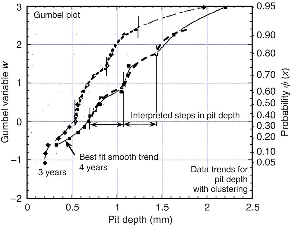
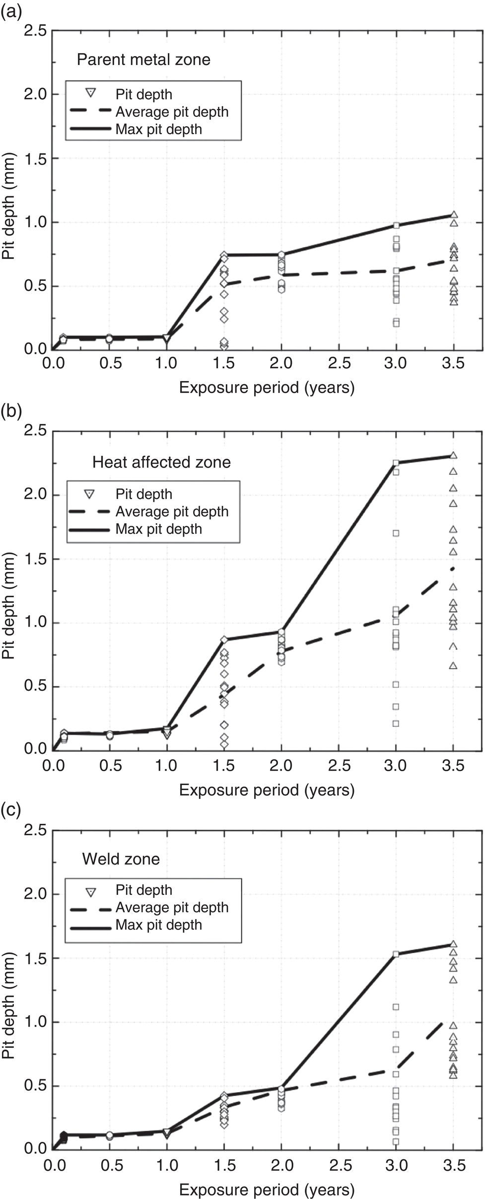
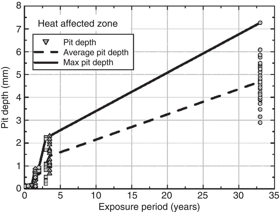
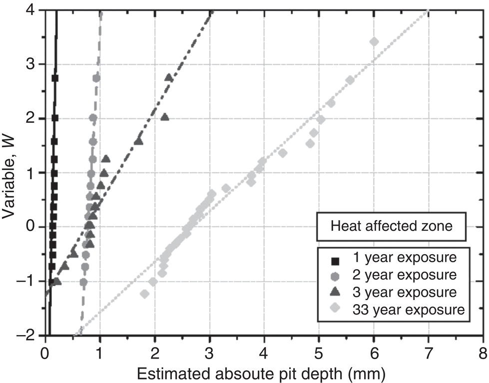
56
Progression of Pitting Corrosion and Structural Reliability of Welded Steel Pipelines
56.1 Introduction
56.2 Asset Management and Prediction
56.3 Pitting
56.3.1 Terminology
56.3.2 Initiation and Nucleation of Pits
56.3.3 Development of Pitting
56.3.4 Biological Influences
56.3.5 Trends in Corrosion with Time
56.4 Model for Long-Term Growth in Pit Depth

56.5 Factors Influencing Maximum Pit Depth Development
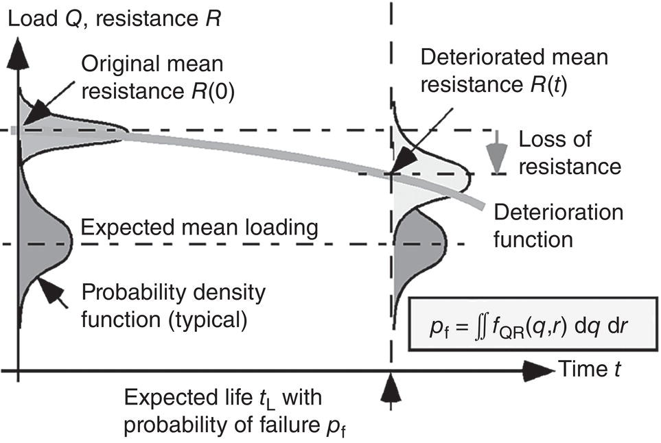
56.6 Structural Reliability
56.6.1 Formulation
Factor
Importance
Factor
Importance
Bacteria/nutrients
High
Pollutants
Varies
Biomass
Low
Temperature
High
Oxygen supply
Short term
Pressure
No
Carbon dioxide
Little
Suspended solids
No
Salinity
Not by itself
Wave action
High
pH
High
Water velocity
High
Carbonate solubility
Low

56.6.2 Failure Conditions

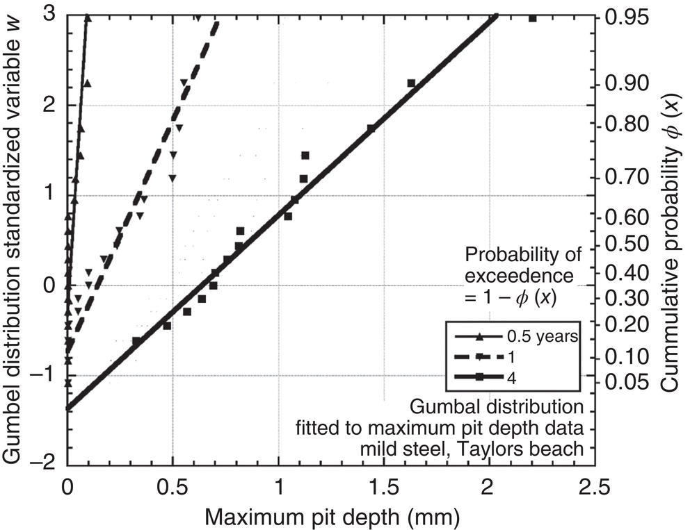
56.7 Extreme Value Analysis for Maximum Pit Depth
56.7.1 Choice of Probability Distribution
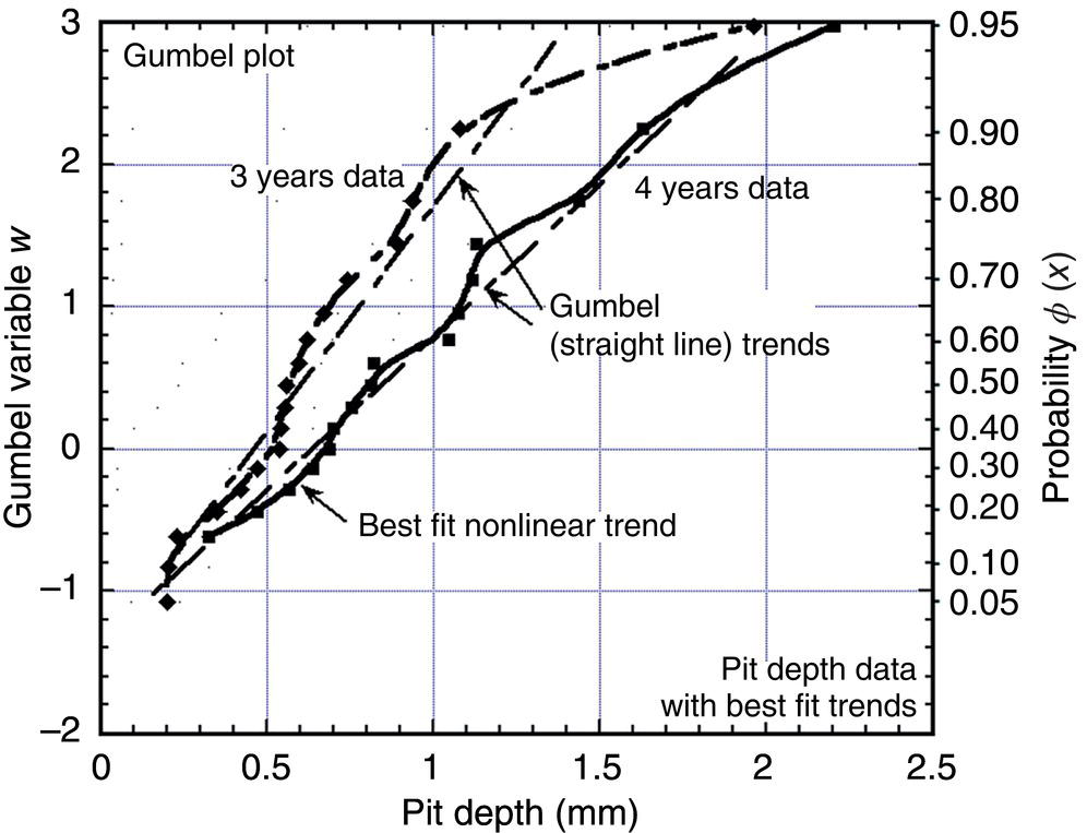
56.7.2 Dependence Between Pit Depths
56.7.3 EV Distribution for Deep Pits
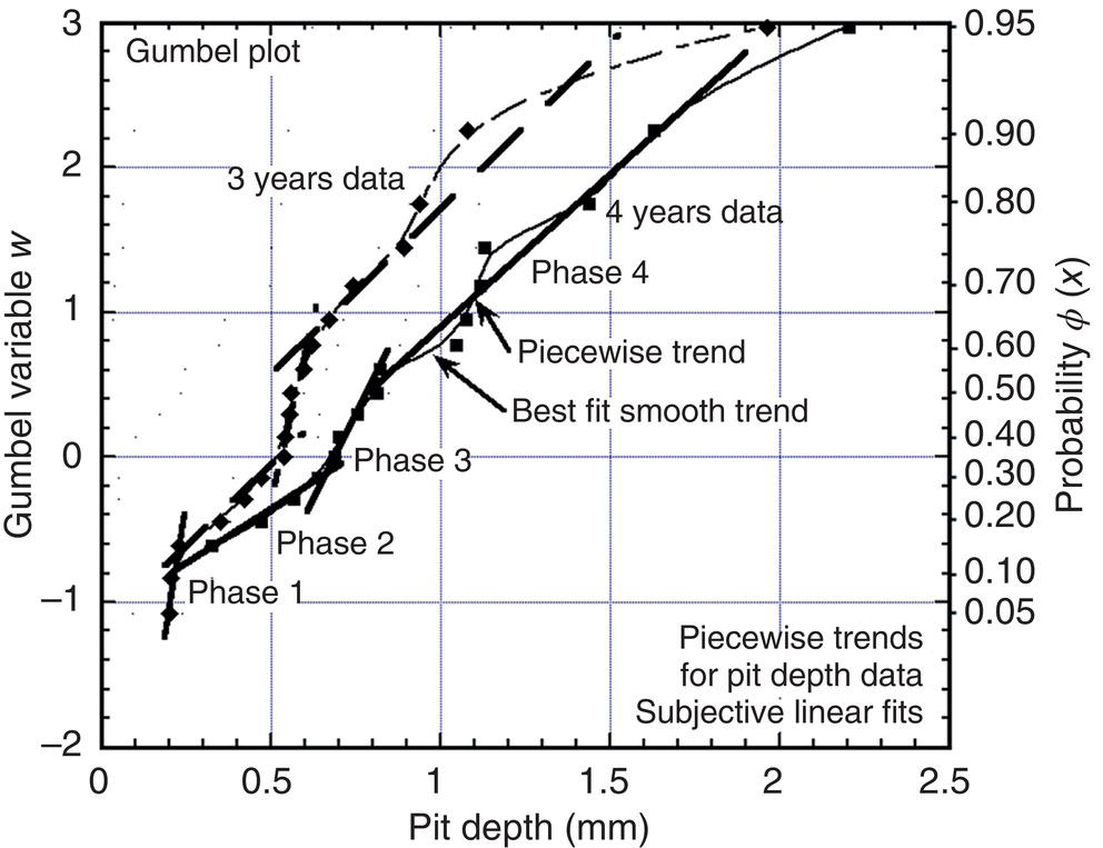
56.7.4 Implications for Reliability Analysis
56.8 Pitting at Welds
56.8.1 Short-Term Exposures
56.8.2 Estimates of Long-Term Pitting Development
Exposure Period (years)
1
1.5
3.5
33
Parent metal
0.10
0.75
1.1
4.9
Heat-affected zone
0.12
0.85
2.3
7.3
Welds zone
0.10
0.40
1.6
5.1
56.8.3 EV Statistics for Weld Pit Depth
56.9 Case Study—Water Injection Pipelines
56.10 Concluding Remarks
Acknowledgments
References
Progression of Pitting Corrosion and Structural Reliability of Welded Steel Pipelines
(56.3)

(56.5)