Douglas Hornbach and Paul Prevéy Lambda Technologies, Cincinnati, OH, USA Residual stresses introduced into pipelines by welding and forming during assembly, installation, or repair and their effect on service life are often overlooked. The goal of this chapter is to provide engineers engaged in the design, installation, and maintenance of pipelines with an overview of residual stresses, how they relate to applied stresses, and their influence on the service performance of pipelines and related applications. Avoiding detrimental tension when possible and dealing with unavoidable tension by thermal stress relief or the introduction of beneficial compression for improved performance are covered. The effects of residual stresses on stress corrosion cracking (SCC) and fatigue failure mechanisms are briefly discussed but are covered in detail elsewhere in this volume. Practical methods of measuring residual stresses that may be of use to a pipeline engineer are included, with an emphasis on their relative advantages and limitations. The effect of cold working and “microstress” upon corrosion behavior is included. Residual stresses, sometimes referred to as “self-stresses” or “internal stresses,” are those stresses that are present in a body when it is free of any externally applied forces. Residual stresses are as real as applied stresses, and will generally be retained in a component, such as a section of welded pipe, assembled coupling, or flange joint for the entire service life. Residual stresses are additive to the applied stresses with which engineers are primarily concerned in the design of a pipeline, and the summation of stress governs performance in service. Tensile residual stresses are generally detrimental, and compressive residual stress can markedly improve performance. The magnitude of residual stresses can often exceed the applied stresses and can therefore have a major impact on the performance in service. Residual stresses can be considered of two types—macroscopic and microscopic, which are distinguishable by X-ray or neutron diffraction. Macroscopic residual stresses extend over distances that are large relative to the size of the crystals or grains of the material, on the order of millimeters. Macroscopic residual stresses are directly additive to the applied stresses, which engineers must consider, due to mechanical loads and pressures on a pipeline. Microstresses are the result of plastic deformation, or cold work, of the metallic material. Microstresses are very local stresses that extend over distances between the dislocations present within the individual crystals in the metal, on the order of fractions of a micrometer. Microstresses can alter material properties, such as yield strength, crack propagation, and corrosion behavior, influencing how the sum of applied stresses and macroscopic residual stresses affect performance. Although the term “cold working” is sometimes used to imply introducing macroscopic residual compression, as by shot peening (SP) or roller burnishing, it is important to realize that there is no definite relationship between macro- and microstresses or residual stress and cold work. Stress is a tensor property, whereas cold work is a scalar property describing the degree of plastic deformation the material has experienced. A body can be uniformly highly cold worked but nearly stress free. Alternatively, simple bending can produce residual stresses equal to the yield strength with very little cold working. The term residual stress, as used here, refers to macroscopic residual stress. Cold work refers to the combination of dislocation density and microstrain causing work hardening. Residual stresses are caused by nonuniform plastic deformation of either thermal or mechanical origin or by localized phase transformations, such as case hardening of steels. The residual stresses remaining once all external loads are removed are necessarily entirely elastic. Regardless of the complex thermal–mechanical history of smelting, rolling, forming, grinding, welding, and whatever may have occurred, the residual stresses remaining after that complex processing will be entirely elastic. The residual stresses are limited to the yield strength of the material in the final cold-worked or heat-treated condition. The strains due to the elastic residual stresses can then be measured by mechanical dissection or diffraction techniques and used to calculate the residual stresses present. Residual stresses encountered in pipelines arise from various sources, such as the original fabrication of the pipe sections, welding, forming, machining, grinding, handling, and even assembling of the pipeline. The final state of residual stress in any section of pipe arises from the differences in the amount of plastic and elastic strains created by the combined thermal–mechanical history. Pipe sections fabricated as rolled, longitudinally welded sections can contain residual stresses from both the forming into the cylindrical shape and the welding of the pipe along the seam [1]. Helical welded pipe will have a more complex stress distribution, again due to the forming and welding. Extruded pipe, although seamless, may have a through-wall stress distribution created in the piercing and drawing operations [2]. Any bending of pipe to form curved sections will produce tensile residual stresses on the inside of the bend (intradose), which is driven into compression during bending, and compressive residual stresses on the outside (extradose) of the bend, which is stretched in tension. Because the highest plastic strain gradient during bending is at the start of the bend, the highest tensile residual stresses are often at the point of tangency just entering into the bend on the inside surface. Flaring or other sizing of pipe or tubing to alter diameter will produce residual stresses that can be in high tension at the point of transition into the increased diameter. Any process that nonuniformly deforms a metal component can result in residual stresses up to the yield strength of the material. Once the external forces are removed, the residual stresses will immediately equilibrate. Tensile residual stresses will be produced in the areas that are plastically deformed in compression during the forming operation; compressive stresses will occur in the regions deformed in tension. The residual stress distribution in any body must be in equilibrium after external forces and tractions are removed. Equilibrium requires that the sum of the moments and forces acting on any plane entirely through the body must be zero. Equilibrium does not imply that there should be equal and opposite residual tension and compression in adjacent locations in a component. For example, a layer of equal magnitude tension does not occur immediately beneath the compressive layer produced by SP a section of pipe. Instead, low-magnitude tension extends through the thick wall to balance the thin compressive surface layer. A region of residual tension may exist through the entire thickness of a component. For example, a pipe wall that has been heated locally so that it deforms in compression entirely through the wall by thermal expansion will leave the heated zone in tension when cooled. The zone of through-thickness tension is then supported in equilibrium by surrounding material in lower magnitude compression. Welded pipe joints are a primary source of residual stress [3]. Welding creates regions that are heated to a liquid or highly plastic state, fused, and then allowed to cool locally. The contraction of the metal upon cooling stretches the fusion zone into high tension, typically up to the yield strength. A zone of residual tension then extends out into the heat-affected zone (HAZ) on either side of the weld [4]. The complex distribution of residual stress, with regions of high tension in a 304 stainless steel T-weld, is shown as a contour plot in Figure 12.1. Multipass welding deposits layers of filler metal that are alternately reheated by the next pass. The result can be complex residual stress distributions created by the partial stress relaxation in the first layer as it is reheated, combined with tension in the newly deposited layer. Preheating the work before welding is a common means of reducing the thermal strain gradient during weld fusion, and thus the tension created when the weld cools. Post-weld thermal stress relief is commonly used to reduce the tensile stresses created by welding, but complete thermal stress relief can be difficult to achieve. To avoid introducing additional residual stresses from thermal strains, the temperature throughout the component must be uniform during the heating cycle. This is especially important in complex welded assemblies where large thermal stress gradients can develop during heating or cooling. Figure 12.2 shows the residual stress depth profiles for a low carbon steel weld before and after stress relief and SP. Because fatigue and SCC initiate at the surface, the stresses produced by finish machining or grinding can be critically important for subsequent performance. Surface integrity is the discipline dealing with how the condition of the surface, including the residual stress and cold work produced by manufacturing, influences performance in service. Machining and grinding produce residual stress distributions that are shallow but can be of very high magnitude [5]. The residual stress layer produced is generally less than 0.25 mm deep, but stresses can reach the yield strength in either tension to compression. Figure 12.1 Contour plot of the surface residual stress distribution in a 304 SS T-Weld. Figure 12.2 Residual stress depth distributions for a low carbon steel-butt weld, after thermal stress relief, and shot peening. Rapid local surface heating is a primary source of highly detrimental residual tension. Machining or grinding practices that quickly heat the surface can produce surface tension and grinder “burn.” The small patch of material at the point of contact with the grinding wheel or cutting tool is quickly heated to incandescence. Local temperatures can be sufficient to cause phase transformations in steels, leaving brittle, cracked, untempered martensite on the surface, a common fatigue initiation mechanism [5]. In any alloy, the locally heated surface zone expands, but is constrained by the cool material below, briefly creating thermal compressive stress sufficient to yield the hot zone in compression. When the tool or grinding wheel moves on, the heated zone rapidly cools by self-quenching into the cool substrate material, stretching the heated zone into residual tension. The residual tension may be so high as to cause surface cracking, forming fatigue and SCC initiation sites. Figure 12.3 shows the residual stresses left behind by “abusive” grinding (with high heat input) of low carbon steel weld coupons. Note the high surface tension. Cold machining or abrasive operations like polishing and gentle grinding typically produce shallow but often high residual compression. A shallow layer of surface compression is produced generally using a liquid coolant so that the surface is not significantly heated. The surface yields in tension as chips are formed and is then left in residual compression as the part returns to equilibrium. “Gentle” milling, turning, and similar chip forming operations performed with coolant, sharp tools, shallow depths of cut, and low feeds that minimize heating also leave a compressive surface layer. Wire brushing generally produces compression if heat is avoided. Figure 12.3 Subsurface residual stress distributions in ground low carbon steel welds. Grinding or machining for the preparation of pipeline welds deserves special mention. Weld preparation by grinding or machining can highly cold work the exposed surface layer, increasing the yield strength of the surface material near the weld fusion zone. Contraction of the weld upon cooling then stretches the cold-worked material in the HAZ into high residual tension, up to the higher yield strength of the cold worked layer, leaving the HAZ subject to fatigue or SCC failure in service. This is a primary cause of SCC failures of 304 stainless steel pipe butt weld joints that were machined or ground to match wall thickness in boiling water nuclear reactor piping. Installation or “fit-up” stresses are sometimes considered residual stresses in the assembled pipeline or component assembly. Stresses from suspending a pipeline with hangers, loss of support caused by erosion, or flexing of pipe sections to make connections before welding or flange joining become residual stresses in the completed assembly. Surface damage during transport, handling, and assembly can produce dents, gouges, cold-worked zones, local areas of high residual stress, and stress concentrations that serve as fatigue and SCC initiation sites [6]. The macroscopic residual stresses of concern to engineers are inherently elastic and are additive to applied stresses. Residual stresses remain in equilibrium in the body indefinitely after creation by thermal–mechanical processes that cause nonuniform plastic deformation. Pipeline stresses from pressurization, suspended loads, pumping vibration, earthquakes, soil settling, and so on are summed with any existing residual stresses in the pipe. Pipeline failures in service are primarily due to fatigue, SCC, or corrosion fatigue (CF), all of which require a net tensile stress at the surface for initiation. Tensile residual stresses from any cause render the pipeline more likely to fail, while compressive stresses are generally beneficial. It is useful to consider how residual stresses influence each of these failure mechanisms separately. Fatigue failure is caused by cyclic loading to stress levels above the endurance limit of the material. Cracks initiate at the surface or from some internal flaw, such as a void or inclusion in the metal. Stress concentrations such as corrosion pits or scratches due to handling are common initiation sites. Fatigue is classified as low cycle fatigue (LCF) or high cycle fatigue (HCF), depending upon the stress level and number of cycles to failure. In LCF, the maximum alternating stress exceeds the proportional limit, causing some local plastic deformation with each cycle. Cracks initiate immediately, and the cyclic life to failure is determined by crack propagation. The LCF cyclic life is usually in tens of thousands of cycles, generally less than 50,000 cycles. Cyclic plastic deformation during LCF reduces the effect of any residual stresses and even the applied mean stresses. HCF occurs more commonly in pipelines, under essentially elastic cyclic loading, and failures occur only after 105 or more cycles. Residual stresses add to the mean applied stress during fatigue and can strongly influence HCF performance. Welding residual stresses have a dominant influence on the mean stress and fatigue performance in pipelines [7]. “Fit-up” stresses created when pipes are aligned during assembly also become residual mean stresses in service. Once a pipeline is assembled and in operation, the vibratory stresses contributing to fatigue are generally so small that only HCF needs to be considered. All fatigue failures initiate in shear, usually at the surface of a body under cyclic load because the shear stresses are maximum at the free surface. When the maximum stress is raised to the fatigue endurance limit, those few crystals on the surface that happen to be favorably oriented to exceed the critically resolved shear stress (i.e., having slip planes tipped 45° into the direction of loading) will begin to ratchet on slip planes with each loading cycle. Dislocations are pumped along the slip planes, alternately forming notches and extruding metal slightly from the surface. After the majority of the fatigue life in HCF, the ratcheting process eventually creates a notch on the order of a full crystalline grain. Fatigue cracks then grow from the notch propagating by the rules of fracture mechanics to failure in the final stages of the fatigue process. The contribution of mean stresses and residual stresses to fatigue performance can be understood in terms of the Haigh diagram. The alternating stress allowed for a given fatigue life is plotted on the vertical axis as a function of the mean stress, plotted on the horizontal axis, which ranges from tension to compression. The sum of the alternating and mean stress is limited to the material yield strength at the triangular boundary. The Goodman line, an estimate for only tensile mean stresses, is plotted from the fully reversed (zero mean stress) fatigue strength to the ultimate strength. An example for P110 steel oil field tubulars for a fatigue life of 107 cycles is shown in Figure 12.4. The Smith–Watson–Topper curve plotted for no damage, kf = 1, gives the upper bound for the allowed alternating stress with mean stresses extended into compression. (The fatigue factor kf is simply the inverse of the fraction of the undamaged fatigue strength remaining.) Adding Neuber’s rule to account for damage provides a fatigue design diagram (FDD) useful for determining the amount of compression needed to mitigate damage [8]. The total mean stress determining fatigue life is the sum of the applied mean stress and the residual stresses at the surface of the pipe. In pipeline applications, the alternating stresses may be the transient stress from vibrations, periodic loading, or pressure pulsations from a pumping station. Figure 12.4 Fatigue design diagram for P110 steel. The FDD shows that under compressive mean stress, applied and/or residual, the allowed alternating stress increases significantly. Damage causing surface stress concentrations increases kf, greatly, reducing the alternating stress allowed for any given positive mean stress. The allowed alternating stress must be less than the kf = 3 curve for a 107cycle life, that is, when damage reduces the fatigue strength to one-third of the undamaged strength. Even with severe damage, such as an existing fatigue crack, if the sum of residual and applied mean stresses moves the operating condition into the gray triangle labeled “SAFE,” then the material is always in compression, and fatigue cracks cannot grow. Any surface, even with fatigue-initiating damage, operating within this safe triangle cannot fail by Mode I crack growth in fatigue. This is the basis for introducing beneficial residual compression using surface enhancement treatments. The maximum possible alternating stress is achieved at the center of the “SAFE” triangle with the net mean compressive stress, residual plus applied, in the damage-prone surface layer equal to half of the material yield strength. SCC refers to the propagation of cracks under a static tensile load in the presence of a chemically active environment to which the material is susceptible. SCC is also termed “environmentally assisted” cracking. Ferritic pipeline steels can be subject to hydrogen sulfide (H2S) SCC or “sulfide stress cracking” (SSC) in sour well environments [9, 10]. Carbonate (CO3) cracking is also possible and chloride SCC is common to many alloys, notably stainless steels, and is exacerbated by tensile residual stresses [11]. Pipelines transporting ethanol, even as a minor fraction mixed with petroleum products, are subject to internal SCC due to the affinity of ethanol for water and the ability of ethanol to support corrosion [12]. The combination of chemical and mechanical elements makes SCC more complex, and less well understood, than fatigue. The mechanisms and occurrence of SCC in various alloys and environments are discussed in detail elsewhere in this volume. SCC can only occur if three conditions are met, as shown schematically in the Venn diagram in Figure 12.5. First, the material must be susceptible to cracking in the service environment. Second, the material must be exposed to the chemically active environment with the ions present that will cause cracking to occur. Third, there must be a tensile stress, residual plus applied, present at the surface of the material that exceeds some threshold level. One possible, but often prohibitively expensive, way to mitigate SCC is to replace the alloy with one that is not susceptible in the environment. In the case of ferritic steels, the use of lower strength grades with higher fracture toughness can reduce the propensity to fracture but with the performance limitations of the lower strength. A protective coating can be used to isolate the surface from the chemical environment, but the coating may be breached, allowing failure. Figure 12.5 Venn diagram of SCC contributors: susceptible material, corrosive environment, and tension. As in the case of fatigue, residual stresses influence SCC by being additive to the mean stresses applied to the pipeline. If a tensile residual stress, for example, from welding, added to the applied stress exceeds the threshold for SCC for that material and exposure, cracking can be expected to occur. Welding procedures and parameters can be modified to control the magnitude and distribution of residual stresses developed by pipeline welding [13]. If the surface that is in contact with the environment is kept in compression by a layer of residual stress, SCC can be eliminated. It may be possible to control welding methods to produce compressive residual stresses in the pipe [14]. In addition to inter- and transgranular SCC cracking, corrosion pitting has been reported to occur preferentially in areas with the highest tensile residual stress [15]. CF is the combination of mechanical fatigue-generated cracks that are further propagated in a chemically aggressive environment by SCC. The fatigue strength of many alloys is reduced by exposure to chloride solutions, generally salt water. In fatigue with the absence of corrosion, many alloys, including pipeline steels, will exhibit an endurance limit. Below this cyclic stress level, fatigue cracks will not initiate, and the fatigue life is essentially infinite. A prominent effect of CF, illustrated in the case studies’ section, is the elimination of any endurance limit so that fatigue cracks propagate even at very low alternating stress levels. In high-strength steels, the loss of fatigue strength in the presence of a corrosive environment can be spectacular. High-strength 300M steel exposed to 3.5% NaCl solution has only 20% of the fatigue strength of baseline material at 107 cycles, with no evident endurance limit. As in simple fatigue or static SCC, the presence of residual stresses adds to the mean stress and can either exacerbate or mitigate CF. The corrosion debit during fatigue in pipeline steels requires tension exceeding a threshold level and is mitigated by reducing tensile or introducing compressive residual stress [15]. Any polycrystalline metal, such as pipeline steel, when mechanically processed by grinding, machining, bending, flaring, weld shrinkage, or other mechanical means will necessarily be plastically deformed to some degree. Even a delicate metallographic polishing process is a chip forming grinding operation on a microscopic scale, plastically deforming the surface to a very shallow depth. Plastic deformation of metals forms vast numbers of dislocations along slip planes in the individual grains or crystals of the metal. The increase in dislocation density changes the properties of the metal in ways that can be as important as the macroscopic residual stresses. During X-ray diffraction residual stress measurement, the degree of plastic deformation can be quantified as an increase in diffraction peak broadening, while the macroscopic residual stress causes a shift in the peak angular position. Cold working influences the corrosion behavior of many metals, leaving the deformed surface more chemically active. For example, cold working of P110 steel casing reduces the open-circuit potential (OCP) in salt water, effectively making the metal less noble than chemically identical P110 material that is not so severely cold worked. The cold-worked areas corrode preferentially and faster than the undisturbed material. The corrosion rates of pipeline steels have been shown to increase with cold working in sour gas (H2S) environments [16, 17]. Cold working influences the stability of residual stresses at elevated temperatures. Once the dislocation density of the material becomes high enough, residual stresses can relax extremely rapidly by dislocation annihilation when the metal is heated. This effect can result in the loss of beneficial compression introduced by SP or other mechanical working processes that introduce high levels of cold work [18]. Cold working and the resulting dislocation density produce an increase in the yield strength of many materials. A surface cold-worked by SP or other means will have a variation in yield strength with depth through the deformed layers, from the highly cold-worked surface to the unworked interior. Austenitic alloys, like stainless steels, can have a 400% increase in yield strength from surface work hardening, as by machining or grinding. If the surface layer of cold-worked metal is then deformed, as may occur in forming tubing or in a weld HAZ during cooling and contraction, the metal will yield different amounts at each depth. The final residual stress distribution then depends upon the original state of residual stress and the yield strength in each layer. A compressive surface layer produced by SP or low stress grinding can be left in residual tension after subsequent deformation. Because cold working can alter mechanical behavior, unnecessary cold working should be avoided. Austenitic alloys with face-centered cubic structures are particularly susceptible to work hardening. Minimizing cold work ensures that the finished pipeline or component will behave in a manner to be expected for the base material properties. This section is intended to introduce the pipeline engineer to the practical methods of residual stress determination that should be considered in the event that measurement is necessary and to support understanding of residual stress studies presented in the literature. The advantages, disadvantages, and limitations of the established methods are described. Methods that have been investigated but remain largely in the laboratory and are of limited use to a pipeline engineer are not included. The reader is referred to handbooks with comprehensive chapters covering the various methods for detailed discussion of the practical techniques and experimental methods [19, 20]. Although commonly used, the phrase “residual stress measurement” is a misnomer. Stress, like density, is an extrinsic property that cannot be directly measured but can only be calculated from measurable properties. Residual stress “measurement” or determination methods can be considered in two categories: those that measure strain and calculate the stress by linear elasticity theory and those that utilize some other property influenced by residual stress, such as magnetic or acoustic behavior. The linear elastic methods that measure strain, or changes in strain, and calculate the stress using elasticity theory include the mechanical and diffraction methods. No matter how complex the thermal and mechanical history of a part may be, the residual stresses once the body is in equilibrium are necessarily entirely elastic. Therefore, the residual strain that can be measured is proportional to the residual stress. The first group of linear elastic mechanical methods includes all of the dissection methods of slitting, sectioning, center hole drilling, and ring core or trepanning that use electrical resistance or mechanical strain gauges to measure the change in strain as residual stresses are relaxed. The residual stresses present before sectioning are calculated from the change in strain caused by sectioning or material removal. Most of the layer removal and slitting methods rely upon simplifying assumptions of component geometry and stress field to facilitate solution. Only the portion of the residual stress that is relaxed by sectioning can be calculated, so the choice of method and sectioning affects the result. Care must be taken not to introduce residual stresses during the sectioning operations. The second group of linear elastic methods includes the X-ray diffraction (including synchrotron) and neutron diffraction techniques. Diffraction methods measure the strain between planes of atoms in the crystals of the material, in this case the pipeline steel. Tension will increase and compression will decrease the lattice spacing in the direction of the residual stress. The residual stress is calculated from the strain measured in the crystal lattice. The diffraction techniques are nondestructive but require sampling of a large number of small crystals to provide an accurate statistical average of the macroscopic residual stress. Measurement in coarse-grained material, such as castings and weld fusion zones, can be difficult. Conventional X-ray diffraction penetration is very shallow, on the order of 0.01 mm, providing only surface values without removing material to expose subsurface layers for measurement. Plane stress can be assumed at the free surface, and therefore, knowledge of the unstress lattice spacing is not necessary. Neutron and synchrotron radiation can penetrate to centimeter and millimeter depths, respectively, but require highly specialized facilities and independent knowledge of the unstressed lattice spacing to calculate the full stress tensor present. Residual stress measurement by mechanical methods involves removing or sectioning material to relieve a portion of the residual stress and measuring the resulting change in strain or dimensions, from which the stress relaxed is calculated. These methods can be categorized as destructive or semidestructive depending upon the relative amount of material removed. Displacements are typically measured with electrical resistance strain gauges. Air gauge and optical systems can also be used to measure dimensional changes. The residual stress that was relaxed by sectioning is then calculated using equations developed by assuming some symmetry to the residual stress field to allow algebraic solution. Both sectioning and hole drilling methods are commonly applied to welded pipelines [21]. For the general application, semidestructive mechanical measurement methods such as center hole drilling and ring core are preferred because symmetry of the residual stress field is not required for solution. Nonlinear elastic techniques form the other major class of residual stress determination methods. These include magnetic and ultrasonic techniques, where pressure- or stress-sensitive changes in properties other than strain are measured. All of these require measurement of some nonlinear, often high-order effect with high accuracy. All are strongly influenced by other material properties, such as hardness, dislocation density, and crystal orientation, so that interpretation of the residual stress contribution is very difficult in practice. The Barkhausen noise magnetic method is the only nonlinear elastic method that will be further considered here [19]. The center hole drilling method [20, 22, 23] is a mechanical technique that allows the determination of bulk or incremental residual stress versus depth. Hole drilling involves introducing a small hole at the center of a specially designed three-or six-element strain gauge rosette and measuring the resulting strain relaxation. A sectional view of the hole and strain gauge arrangement is shown schematically in Figure 12.6a. Figure 12.6b shows a photograph of measurement on a butt-welded pipe. Depths of up to 2 mm (0.08 in.) can typically be measured with this method. The hole drilling method is often referred to as semidestructive because the hole that is introduced may not significantly affect the usefulness of the work piece for some applications or may be repaired after measurement. It has been used extensively for both laboratory and field studies of residual stresses, including welding stresses in pipe [21]. Figure 12.6 (a) Schematic of center hole drilling test, (b) example of incremental center hole drill residual stress measurement on a butt-welded pipe sample. Figure 12.7 Example of hole drilling data set. Principal residual stresses and their angular orientation are determined from the relaxed strain using calibration coefficients for each specific strain gauge geometry and hole size. An example of the subsurface principal residual stress distributions produced by low plasticity burnishing on a test coupon and measured by the incremental center hole drilling method is shown in Figure 12.7. The hole drilling procedure has been standardized in ASTM Standard Test Method E837 under the auspices of Subcommittee E28.13 on residual stress measurement [22]. This method is applicable when the material behavior is linear elastic. When the residual stress exceeds nominally half of the yield strength, it is possible in theory for local yielding to occur due to the stress concentration formed by the drilled hole. Then, stresses calculated to be significantly higher than half the yield strength may be subject to experimental error. The theoretical basis, underlying assumptions and limitations, are most thoroughly developed in Micro-Measurements Tech Note TN-503, which is strongly recommended as a training guide [23]. Hole-drilling equipment and supplies are commercially available and a qualified stress technician can successfully perform the test by adhering to the ASTM standard. Tests can be performed either in a laboratory or in the field on components with various sizes and shapes. The ring core or trepanning [19, 24, 25] is another mechanical residual stress measurement method that allows for residual stress measurements to be made at greater depths than the hole drilling method. The ring core method involves introducing an annular groove around a three-element strain gauge rosette. Because the cylindrical core is completely separated from the surrounding material, more of the residual strain is relaxed, and the ring core technique can provide nominally an order of magnitude greater measurement sensitivity than hole drilling. The stress in the cylindrical core containing the strain gauge is relaxed and the resulting strain relaxations are measured. Because there is no stress concentration at the gauges on the cylindrical core, residual stresses can be measured accurately up to the yield strength. Principal residual stresses and their angular orientation at each depth are determined from the relaxed strain using relaxation coefficients determined by calibration or finite element calculation. Figure 12.8a shows a schematic, in section, of the basic ring core setup, and Figure 12.8b shows a photograph of ring core measurement on a plate. Figure 12.8 (a) Schematic of ring core test, (b) incremental ring core residual stress measurement on plate sample. Depths of up to 5 mm (~0.2 in.) can typically be measured in a single diameter ring core operation. Measurement depth can be increased through the use of larger diameter coring tools; however, resolution is reduced as a trade-off. Because the strain response attenuates with greater depths, there is a limit to which residual stresses can be measured. In order to collect deeper residual stresses, the cylindrical post can be removed and a new strain gauge applied to continue further in depth. An example of the principal residual stress distributions measured by the incremental ring core method in a welded 304 SS sample is shown in Figure 12.9. Figure 12.9 Example of ring core subsurface residual stress data set. The slitting method [20, 26, 27] is a mechanical residual stress measurement technique that measures through-thickness residual stress in a single direction. The slitting method is also referred to as the crack compliance method. This type of measurement is typically used on test pieces with a uniform cross section along the length of the piece and is limited to measuring the in-plane normal stress in one direction. The method involves introducing a slit into the test piece, typically using wire EDM, containing at least one uniaxial strain gauge on the side opposite the cut start side. Additional strain gauges can be used to improve measurement sensitivity. Strain relaxation is monitored with incremental slit depth via the strain gauge/s from which the resulting residual stress distribution is determined using a geometry-specific, finite element-based compliance matrix. Figure 12.10a shows a schematic of a slitting/slotting setup. Figure 12.10b shows a photograph of slotting measurement at the edge of a weld fusion zone. Figure 12.10 (a) Schematic of slitting/slotting, (b) example of incremental slotting residual stress measurement on welded plate sample. Figure 12.11 Example of a slitting/slotting data set. More recently, a test method referred to as the slotting method was developed, which combines aspects of the slitting method with previously described near-surface mechanical methods. Slotting is used to characterize near surface residual stresses much like the hole drill and ring-core techniques. As is the case with slitting, the slotting method allows for measurement of a single in-plane normal residual stress. Slotting measurements are carried out by machining a localized slot, typically using an end-mill via CNC control, into a test piece instrumented with a uniaxial strain gauge adjacent to the slot. Strain relaxation is collected incrementally with depth to allow for calculations of incremental near-surface residual stresses at depth increments on the order of the hole drill and ring core methods. The slotting method can be used on an array of component geometries and sizes. Figure 12.11 shows an example of a slitting/slotting data set. The Deep Hole Drill (DHD) [28, 29] method is a mechanical residual stress measurement technique that allows for the measurement of relatively deep stresses without the need for instrumenting the test piece with a strain gauge. Originally designed and used in rock mechanics, the method has been expanded for use on an array of engineering materials with specific emphasis on metal alloys. Due to its unique capabilities compared to other mechanical methods that use surface mounted strain gauges, DHD can provide the principal residual stresses and their orientation hundreds of millimeters into a part for applications that require knowledge of the through-thickness stress state. Figure 12.12a shows a schematic of DHD. Figure 12.12b shows an example of through-wall incremental DHD residual stress measurement on thick plate. The method of using DHD on metals generally consists of first drilling a reference hole through the test piece. Gun drilling is often the method of choice to introduce the reference hole due its ability to create deep holes with optimal straightness and uniform diameter. Diametral measurements are then collected incrementally with depth on the inside diameter of the reference hole using an air-gauge along the entire length. Following the diametral measurements, the reference hole is overcored to release it from the test piece, consequently changing the hole shape due to local relaxation of the residual stress. Diametral measurements are again made on the reference hole following the overcore process and compared to the initial measurements to determine the change in diameter. Finally, the residual stresses are calculated at each of the measured depths using equations derived from linear elastic solutions for a hole in a stressed plate and the changes in reference hole diameter. Figure 12.13 shows an example of a DHD data set. In X-ray diffraction residual stress measurement, the strain in the crystal lattice is measured directly and the residual stress producing the strain is calculated, assuming a linear elastic distortion of the crystal lattice. Recall that all residual stresses are necessarily elastic. The basic “sine-squared psi” method was well developed by the SAE Fatigue Design and Evaluation Committee in the 1960s, and the reader is referred to SAE HS784 for details of the theoretical basis and practical experimental techniques [30]. XRD is the only nondestructive method that determines residual stress directly from measured strain and can be used in the field or laboratory with commercially available apparatus. The pipeline engineer interested in determining residual stress will benefit by understanding the similarity of XRD to mechanical elasticity-based methods. Therefore, a brief overview with derivation from linear elasticity theory is presented. Figure 12.12 (a) Schematic of deep hole drilling, (b) example of through-wall incremental deep hole drill residual stress measurement on thick plate. Figure 12.13 Example of DHD data set. X-ray diffraction residual stress measurement is applicable to materials that are crystalline and relatively fine grained so that measurable diffraction peaks are produced for any orientation of the sample surface. To determine the stress, the strain in the crystal lattice must be measured for at least two orientations relative to the sample surface. Samples may be metallic or ceramic, provided a diffraction peak of suitable intensity and free of interference from neighboring peaks can be produced in the high back-reflection region with the radiations available. X-ray diffraction residual stress measurement is unique in that macroscopic and microscopic residual stresses can be determined nondestructively and separately from the diffraction peak position and breadth, respectively. Figure 12.14 shows the diffraction of a monochromatic beam of X-rays at a high diffraction angle (2θ) from the surface of a stressed sample for two orientations of the sample relative to the X-ray beam. The angle ψ, defining the orientation of the sample surface, is the angle between the normal of the surface and the incident and diffracted beam bisector, which is also the angle between the normal to the diffracting lattice planes and the sample surface. Diffraction occurs at an angle 2θ, defined by Bragg’s law: nλ = 2d sin θ, where n is an integer denoting the order of diffraction (typically, n = 1), λ is the X-ray wavelength, d is the lattice spacing of crystal planes, and θ is the diffraction angle. For the monochromatic X-rays produced by the metallic target of an X-ray tube, the wavelength is known to high accuracy, on the order of 1 part in 105. Strain from residual stress in the material causes small changes in the lattice spacing, d, and a corresponding shift in the diffraction angle 2θ. The strain can be calculated from the measured shift in diffraction peak position. Figure 12.14a shows the sample in the ψ = 0 orientation. The presence of a tensile stress in the sample results in a Poisson’s ratio contraction of the planes parallel to the surface (and thus oriented to diffract), reducing the lattice spacing, and slightly increasing the diffraction angle 2θ. If the sample, or apparatus, is then rotated through some known angle ψ (Figure 12.14b), the tensile stress at that angle increases the lattice spacing of the regions diffracting at that angle and decreases the diffraction peak position, 2θ. The change in the angular position of the diffraction peak measured for at least two orientations of the sample defined by the angle ψ enables calculation of the stress present in the sample surface. The stress direction is in the plane of diffraction, the plane that contains the incident and diffracted X-ray beams. To measure the stress in different directions at the same point, the sample is rotated about the surface normal to bring the direction of interest into the diffraction plane. Figure 12.14 Principles of X-ray diffraction stress measurement. (a) ψ = 0, (b) ψ = ψ (sample rotated through some known angle ψ). D: X-ray detector; S: X-ray source; N: normal to the surface. The residual stress determined using X-ray diffraction is the arithmetic average stress in a volume of material defined by the irradiated area, which may vary from square centimeters to square millimeters, and the depth of penetration of the X-ray beam. The linear absorption coefficient of the material for the radiation used governs the depth of penetration, which can vary considerably. In steels, 50% of the radiation is diffracted from a layer approximately 0.005 mm (0.0002 in.) deep for the Cr Kα radiation generally used for stress measurement. Electropolishing is used to remove thin layers to expose new surfaces for subsurface measurement with high depth resolution. X-rays used for diffraction residual stress measurement penetrate a very shallow layer of sample material. Therefore, the measured surface is necessarily in a state of plane stress. That is, a stress distribution described by principal stresses σ1 and σ2 exists in the plane of the surface, and no stress is assumed perpendicular to the surface, σ3 = 0. However, a strain component perpendicular to the surface, ε3, exists as a result of the Poisson’s ratio contractions caused by the two principal stresses, shown in a three-dimensional view in Figure 12.15. The strain, εϕψ, in the direction defined by the angles ϕ and ψ is where E is the modulus of elasticity, v is the Poisson’s ratio, and σϕ is the stress of interest in the surface. Figure 12.15 Plane stress elastic model at free surface. If dϕψ is the spacing between the lattice planes measured in the direction defined by ϕ and ψ, the strain can be expressed in terms of changes in the linear dimensions of the crystal lattice: where d0 is the stress-free lattice spacing. Substituting for strain in the crystal lattice, the lattice spacing for any orientation, then, is This is the fundamental relationship between lattice spacing and the biaxial stresses in the surface of the sample. The elastic constants (1 + v)/E(hkl) and (v/E)(hkl) are not the bulk values, but the values for the crystallographic direction normal to the lattice planes in which the strain is measured, as specified by the Miller indices (hkl). Because of elastic anisotropy, the elastic constants in the (hkl) direction commonly vary significantly from the bulk mechanical values. The lattice spacing dϕψ is then a linear function of sin2ψ. If the lattice spacing is measured at two or more angles ψ (“two-angle” or “sine-squared-psi” methods), then the slope of the plot is Solving for the stress of interest, σϕ, is The X-ray elastic constants can be determined empirically, but the unstressed lattice spacing d0 varies with alloy composition, heat treatment, and cold working, and is generally unknown. However, because for metals, E ≫ (σ1 + σ2), the value of dϕ=0 differs from d0 by not more than ±1%, and σϕ may be approximated to that accuracy using: The method then becomes a differential technique and no stress-free reference standards are required to determine d0 for the biaxial stress case. This is a significant advantage over synchrotron and neutron diffraction methods that must assume a three-dimensional stress state and therefore require independent knowledge of the unstressed crystal lattice spacing in order to calculate the stress tensor from the measured strains. Because the depth of material sampled is very shallow, any secondary abrasive treatment, such as polishing, wire brushing or sand blasting, introduces surface residual stresses, generally producing a shallow, highly compressive layer completely altering the original residual stress distribution. Therefore, care must be taken not to alter the residual stresses during sample cleaning and preparation. To measure inaccessible locations, such as the inside surface of pipes and tubing, the sample must be sectioned to provide clearance for the diffraction apparatus and the incident and diffracted X-ray beams. Unless prior experience with the sample under investigation indicates that no significant stress relaxation occurs upon sectioning, electrical resistance strain gauge rosettes should be applied to the measurement area to record the strain relaxation that occurs during sectioning. Following X-ray diffraction residual stress measurements, the total stress before sectioning can be determined by subtracting the sectioning stress relaxation from the X-ray diffraction results. Geometric precision is required for diffraction techniques. Because the diffraction angles must be determined to accuracies of nominally ±0.01°, the sample must be positioned in the X-ray beam at the true center of rotation of the ψ and 2θ axes and the angle ψ must be known and constant throughout the irradiated area. Precise positioning of the sample to accuracies of approximately 0.025 mm (0.001 in.) is critical. The size of the irradiated area must be limited to an essentially flat region on the sample surface. Instrument alignment requires coincidence of the θ- and ψ-axes of rotation and positioning of the sample such that the diffracting volume is centered on these coinciding axes. Instrument alignment can be checked readily using a stress-free powder sample [31]. If the diffraction apparatus is properly aligned, a loosely compacted stress-free powder sample should indicate not more than ±14 MPa (±2 ksi) apparent stress. Excessive sample surface roughness or pitting, curvature of the surface within the irradiated area, or interference of the sample geometry with the diffracted X-ray beam can result in systematic error. Residual stress generally cannot be measured reliably using X-ray diffraction in samples with coarser grain sizes, as are common in castings and weld fusion zones. A major source of potential systematic proportional error arises in determination of the X-ray elastic constants E/(1 + v)(hkl). The residual stress calculated is proportional to the value of the X-ray elastic constants, which may differ by as much as 40% from the bulk value due to elastic anisotropy in the crystal lattice. The X-ray elastic constant can be determined empirically by loading a sample of the material to known stress levels and measuring the change in the lattice spacing as a function of applied stress and ψ tilt [32, 33]. The X-ray elastic constant can then be determined by least-squares regression from the slope of the change in lattice spacing as a function of applied stress. X-ray elastic constants for many alloys and steels have been published. X-ray diffraction measures the entire strain present before any sectioning or removal of material, but the shallow penetration requires removal of layers of material by electropolishing for subsurface strain measurement. There are then two important corrections that must be applied to subsurface measurements. First, in the presence of a steep stress gradient, as is common on machined or ground surfaces, the exponential attenuation of X-rays penetrating the layers of varying stress gives a weighted average stress that can be unfolded if measurements are made in sufficiently fine layers. Second, the removal of stressed material alters the residual stress in the exposed layers, causing an error that accumulates with depth, but can be corrected with an integral solution analogous to the layer removal mechanical residual stress measurement methods. Appropriate corrections for both sources of error in subsurface measurement are well-established and are described with analytical solutions in SAE HS784 [30]. Conventional X-ray diffraction stress determination uses low-energy, shallow-penetrating radiation allowing stress determination in the biaxial case, eliminating the need for a stress-free reference sample to calculate the residual stress. This is a major advantage, allowing reliable measurement in materials, such as welds, with local variation in composition. In principle, the full tensor can be determined nondestructively using either high-energy synchrotron X-radiation or thermal neutrons from a suitable reactor source. Both synchrotron X-ray and neutron diffraction methods have been developed for determining the full triaxial stress tensor [20]. Penetration depths can range from millimeters for synchrotron X-rays to centimeters for thermal neutrons. Both require expensive stationary facilities generally available only at major government laboratories. In all other respects, both are diffraction techniques measuring lattice strain, and are subject to the same limitations and error sources as the conventional, portable, plane stress biaxial X-ray method. Determination of the triaxial stress tensor requires independent knowledge of the unstressed lattice spacing d0 at the accuracy required for strain measurement (1 part in 105) to calculate the residual stress from the measured strains. It is not possible to solve for three-dimensional stresses from the measured strains without separate knowledge of the unstressed lattice spacing as a zero-stress reference. Unfortunately, the unstressed lattice spacing varies with cold working (due to dislocation density), heat treatment, and local variation in chemical composition. In many cases, including surfaces plastically deformed by machining, weld fusion and HAZs, or in case-hardened carburized steels, the lattice spacing varies as a result of deformation, composition, or heat treating, precluding independent determination of the unstressed lattice spacing with sufficient precision to make reliable stress tensor calculations. The equipment requirements, lack of portability, extensive data collection required, and dependence on absolute knowledge of d0 limit the full tensor method primarily to research applications. Mechanical methods, primarily center hole drilling, slitting, and ring core, or conventional plane stress biaxial X-ray diffraction methods, are recommended for general use for determining the residual stress distributions in pipelines. The Barkhausen Noise method [20, 34] is a nondestructive, high-speed technique applicable to ferritic materials and, therefore, well suited for steel pipe inspections [4]. The Barkhausen technique relies upon analyzing the “noise” observed on the magnetic hysteresis loops when an alternating current is used to rapidly magnetize the ferritic metal in different orientations. A pickup coil then detects the resultant magnetic field. The individual magnetic domains within the crystalline grains that make up the material are typically oriented in alternating N–S and S–N orientations. Under stress, the domains can flip their orientation, resulting in changes in the magnitude of the noise imposed upon the magnetic hysteresis loop, shown schematically in Figure 12.16. This noise must be analyzed by electronically separating and filtering a certain noise frequency range that is sensitive to stress. As noted below, the noise level is affected by various other metallurgical properties, such as hardness, grain size, and texture (preferred orientation), the effects of which must be separated from that of residual stress. Figure 12.16 Barkhausen noise caused by magnetic domain reversals on the magnetization hysteresis curve for steel. (Reference [19]/Reproduced with permission of Fairmont Press.) The Barkhausen noise level is expressed as a “magnetoelastic parameter” (MP), defined as the root mean square (RMS) level of the Barkhausen noise after amplification and filtering, relative to the unstressed state of the material. The depth of penetration is governed by the “skin” effect: the strength of the signal is attenuated exponentially with depth and the thickness of the layer of the material sampled diminishes with increasing frequency. Excitation frequencies from 3 to 15 kHz provide a depth of penetration of nominally 0.20 mm. Higher frequencies of 70–200 kHz sample shallower depths on the order of 0.02 mm. Barkhausen provides a sampling depth between that of the shallower X-ray diffraction and the deeper hole drilling or ring core mechanical techniques. The maximum depth of penetration reportedly ranges from 0.10 to 3.0 mm for the practical frequencies and instrumentation. The Barkhausen noise response to stress is asymmetric, being larger for tensile stresses and less sensitive to compression. The response curve is a general sigmoid “S” shape, shown in Figure 12.17. The MP is higher for softer, more easily magnetized low-strength steels, and lower for harder, higher strength steels. Calibration is required for the material, frequency, noise analysis (filtration) method, and instrumentation used. Individual transducers may not be interchangeable, so calibration using strain gauge instrumented beams or pipe sections loaded to known stress levels is recommended for each instrument, material, and application. The Barkhausen technique is sensitive to a range of material properties other than strain, as is true of virtually all of the nonlinear-elastic measurement methods. Barkhausen is sensitive to the grain size of the material. For fine-grained material, the MP initially increases rapidly with grain size, and then less rapidly for larger grains. Texture, or the crystallographic orientation, strongly influences the Barkhausen technique, because it samples the switching of the direction of magnetization of magnetic domains along the specific crystallographic directions. Hardness and yield strength of the material have a strong influence, as shown in Figure 12.17. The hardness dependence is so pronounced that the same Barkhausen technology used for stress measurement is used to distinguish hardness and detect grinder burn in steels. The MP level for a given tensile stress can vary by nearly a factor of 4, from a high output of 200 for soft 35 HRC steel, to as low as 50 for fully hardened 60 HRC material. The dependence on material properties other than stress makes use of the Barkhausen technique highly material and component geometry specific. Figure 12.17 Barkhausen MP calibration curves for steels of different hardness and yield strength showing nonlinearity, higher sensitivity to tensile stress, and reduced sensitivity at higher strengths. Calibration of the Barkhausen probe is necessary to account for the effect that hardness, texture, grain size, and other material properties have in the presence of a varying residual stress field. In the case of pipe, a calibration tool can be made using a section of the pipe instrumented with electrical resistance strain gauges to provide a means of measuring the MP as a function of applied stress. In the case of welds, where there is a wide range of grain size, hardness, and even composition within the weld HAZ, none of the nonstress properties can be assumed to be constant, and interpretation of the Barkhausen data must be used with caution. Rapid detection of potential zones of tension may be then confirmed by other residual stress measurement techniques such as X-ray diffraction or hole drilling. The Barkhausen magnetic method can be summarized as (1) being applicable only to ferromagnetic materials, (2) limited to measuring surface layers of the material, (3) limited in measurement range by saturation of the Barkhausen noise response when testing compressive residual stresses, particularly in hard steels, and (4) sensitive to various microstructural variations (grain size, hardness, and texture), making separation of those contributions from stresses difficult [34]. The engineer has various tools for modifying the residual stresses that are encountered in order to reduce or eliminate the adverse effects of tensile residual stress. Machining and grinding practices can be modified to avoid surface tension, particularly in weld prep areas. Weld shrinkage-induced tension can be reduced by well-established practices of preheating or post weld thermal stress relief. However, it is also possible to introduce beneficial residual compression using surface enhancement methods to further improve performance beyond that achievable with the available materials, even in a stress-free state. When material substitution is not an option, and applied stresses cannot be reduced, surface enhancement can ensure reliable performance, especially in highly stressed critical locations. Several of the available surface enhancement methods are briefly described. SP is the most widely used surface enhancement method. Metallic or ceramic shot, ranging in size from nominally 0.25 mm (0.010 in.) to as large as 3.18 mm (0.125 in.), impacts the surface of the component, producing spherical indentations. The SP process forms a compressive layer through a combination of subsurface compression developed by Hertzian loading combined with lateral displacement of the surface material around each of the dimples. As the dimples overlap with random impacts, the entire surface is effectively elongated, driving the surface layer of deformed material into residual compression as its expansion is resisted and supported by the equilibrating tension in the material below. Metallic shot is often either cast steel or cut wire that has been blasted against a carbide plate to form a nearly spherical shot. Cut wire shot can be manufactured from virtually any alloy to avoid elemental contamination. Ceramic shot is typically zirconium oxide or glass bead. The shot will wear and fracture during use; therefore, the SP media should be constantly screened to remove broken shot and dust. The SP process is defined by parameters that include the size and type of shot used, the Almen intensity achieved, and the coverage. Almen intensity is a measure of the deflection of the Almen A, C, or N strip that occurs during the peening cycle and is a measure of the elastic energy stored in the 1070 steel Almen strip by the formation of a layer of residual compression. Almen intensity is only a SP process control tool. The Almen strip arc height is related to the area under the residual stress depth curve in the Almen strip, and it does not uniquely define a depth or magnitude of compression in either the strip or the component being shot peened. Coverage is the percentage of the surface impacted by shot and is a function of time under the shot stream. To ensure uniform treatment of the surface, coverage is often specified at 100% or higher, implying that each point on the surface was impacted at least one or more times. The shot is accelerated to sufficient velocity to deform the surface on impact either by air blast or wheel machines. In wheel SP machines, the shot is thrown from a rapidly spinning radially bladed wheel. Air blast machines propel the shot in a stream of compressed air through a hardened carbide nozzle. Flapper peening is a form of controlled SP without free flying shot. The flapper tool has captive shot embedded, like rivets, in rubberized fabric flaps that are attached radially to rotate around a shaft. The shaft is rotated so that the flaps successively impact the surface, peening a local area. Flapper peening is typically used for repair or limited access work, or when free shot cannot be tolerated, as in field-welded joints in pipelines [35]. By its very nature, SP relies upon random impacts of shot. In order to achieve the coverage requirements, some regions will receive numerous impacts before adjacent areas are impacted at all. The result is a nonuniform and often very highly cold-worked surface, especially for high coverage peening. Cold work levels range from 40 to over 100% during creation of the layer of surface compression. In the work hardening materials, such as austenitic alloys, peening-induced cold working can exhaust the ductility of the material, leaving a brittle surface layer. SP damage in the form of “laps and folds” creates surface stress concentrations that can reduce fatigue performance. SP is a very practical surface enhancement method, provided the components are not exposed to elevated temperatures or mechanical overload. Research has shown that the highly cold-worked shot-peened surface will relax more completely and much faster than a low cold-worked surface at the same state of compressive stress [18]. In roller or ball burnishing, a wheel-like axle-mounted roller or a hydrostatically supported ball is pressed against the surface. The tool is then moved over the surface, repeatedly deforming the surface layer to create compression up to nominally 1 mm, or more, deep. Like SP, the compressive residual stress-creating mechanism is a combination of subsurface yielding by Hertzian loading and lateral displacement of the surface material. Conventional roller burnishing deliberately creates a highly cold-worked layer that is also in high residual compression. Roller burnishing is generally performed in lathe operations, advancing the tool with each revolution at a constant feed rate. Low plasticity burnishing differs from conventional roller and ball burnishing primarily by imparting the minimal amount of cold working needed to create the depth and magnitude of residual compression required to achieve the desired damage tolerance and fatigue or stress corrosion performance. Low cold work provides both thermal and mechanical stability of the beneficial residual compression. The burnishing force can be optimized for each application and varied under CNC closed-loop control to impart the depth and magnitude of compression required in just the critical failure-prone locations. By controlling the burnishing force, low plasticity burnishing can produce a depth of compression ranging from a few thousandths of an inch to over a full centimeter under closed-loop control. The laser shock peening process introduces compression with low cold working using shock waves to yield the material. Laser peening utilizes high-speed, high-powered lasers to focus a short-duration energy pulse on a coating, usually black tape, on the surface of the work piece to absorb the energy of the laser beam. A transparent layer of flowing water covers the tape to direct the shock wave energy into the surface of the material. When the laser is fired periodically, the laser beam passes through the water, explodes the tape, and creates a shock wave sufficient to deform the surface layer of material. The shocking process is repeated in a computer-controlled pattern across the surface, creating a series of slight indentations and regions of residual compression. Several cycles or “layers” of laser peening are usually required to achieve compressive depths on the order of a millimeter. Although limited by cost, quality control, and logistical issues, laser peening has been studied as a means of introducing residual compression in pipelines and the residual stress distributions documented [36]. Figure 12.18 shows subsurface stress profiles for each surface treatment process and the cold work induced in titanium alloy Ti-6Al-4V. Figure 12.18 Stress profiles and cold work from SP, LPB®, and LSP in Ti-6Al-4V. Thermal stress relief is widely used to reduce residual stresses. Postweld heat treatment of pipeline joints reduces the detrimental tensile stresses generated by welding. The reader is referred to the API bulletin 939E for a detailed discussion of procedures for postweld heat treatment of pipe sections. The primary process at work in thermal stress relaxation is a creep mechanism. Residual stresses relax exponentially with both time and temperature, reducing the overall strain energy. Both tensile and compressive residual stresses are reduced as the temperature of the material is increased. No stresses higher than the yield strength at the maximum exposure temperature can be retained in the component. The conventional rule of thumb for thermal stress relief of steels, based upon this time–temperature relaxation mechanism, is exposure to 611 °C (1150 F) for a period of 1 h for each 25 mm (1 in.) of thickness, with the minimum of 1 h for any thickness being stress relieved. Another mechanism more recently recognized is the rapid relaxation of residual stress in a highly cold-worked material [37]. At elevated temperatures, the deformed surface of machined, ground, shot-peened, and other surfaces that have high dislocation density can relax virtually immediately by a dislocation annihilation mechanism, which is then followed by the slow exponential relaxation. This effect can cause a loss of beneficial compression from SP with elevated temperature exposure, particularly in austenitic alloys. Residual stresses do not relax uniformly, that is, not in proportion to the original levels present at each point in the body, because the amount and rate of stress relaxation depend upon the initial local stress magnitude. Furthermore, the residual stress distribution will reequilibrate as the regions of higher tension or compression relax more rapidly, and by a greater amount, than the lower stress regions. Stresses may increase in some areas following thermal stress relief as more highly stressed regions relax and the stress distribution in body maintains equilibrium. Because the rate of relaxation depends upon the stress level, complete thermal stress relief is nearly impossible to achieve. Once the stresses are reduced, the driving force for further relaxation diminishes, and some level of stress is invariably retained. Successful thermal stress relief requires uniform temperature throughout the component during the process. If large thermal strains are created during either the heating or the cooling stages of the thermal cycle, the plastic strains introduced at elevated temperatures can result in even higher residual stresses after cooling than were present before heating. Quenching from elevated temperatures is an extreme case of high thermal strain, and the source of residual “quench stresses.” Complex geometries such as heat exchangers require very slow heating and cooling to avoid thermal stresses. It may be impossible to thermally stress-relieve components composed of dissimilar materials with different coefficients of thermal expansion. The key to successful thermal stress relief is to keep the entire body at a nominally uniform temperature, which is slowly raised to the critical temperature, held for the required exposure time, and then cooled back to ambient temperature without creating thermal strains that could cause plastic deformation. Thermal stress relaxation can only reduce the magnitude of undesirable residual stresses, but cannot introduce beneficial compression to advantage, and usually must be applied to all or large portions of a component to avoid creating large thermal strains. Mechanical surface enhancement treatments introduce beneficial compressive residual stress locally to eliminate detrimental tension or improve performance at the high-stress critical locations. The following case studies provide examples of use of surface enhancement to mitigate SCC and improve fatigue performance in pipeline-related applications. Corrosion pits commonly form at the site of inclusions on the material surface. Pits can be rounded or branched as the pit grows into the surface and forms fatigue crack- initiating stress concentrations. Corrosion pitting damage generally increases with time. The fatigue debit from pitting is typically on the order of half of the fatigue endurance limit of the material. The fatigue strength can be restored by introducing a layer of compressive residual stress that is deeper than the corrosion, preventing fatigue crack growth from the bottom of the pits. The effect of introducing compressive residual stress on fatigue performance was studied for 4340 steel with corrosion pitting in a salt fog chamber [38]. The benefits of surface enhancement were investigated with fatigue tests conducted in four-point bending at a stress ratio Smin/Smax = 0.1 after exposure to salt fog for 100 and 500 h. Samples were tested with and without wire brushing to remove the corrosion product, as might be performed during maintenance. Residual stress distributions measured by X-ray diffraction are shown in Figure 12.19. Surfaces were low-stress ground, glass bead peened, and low plasticity burnished. Low stress grinding is the common baseline condition for fatigue sample preparation, producing shallow compression typical of cold abrasion processes. Glass bead peening produced an equally shallow (0.05 mm) layer of higher −600 MPa magnitude. Low plasticity burnishing produced a layer of compression over 1 mm deep starting at over −1000 MPa on the surface. The fatigue results in Figure 12.20 show that pitting from 100 and 500 h salt fog exposures reduced the 107 cycle fatigue strength by nominally 25 and 50%, respectively. Fatigue cracks initiated in corrosion pits in all cases. Low plasticity burnishing (LPB®) applied to the corroded surfaces after superficial cleaning to remove loose corrosion product restored the fatigue strength to 110% of the original strength after 100 h exposure and 85% after 500 h. The relative fatigue strength at 107 cycles, summarized in Figure 12.21, is attributed to the increased depth of pitting with exposure time. Fretting damage causes fatigue failures in components that are clamped together and vibrate, such as bolted flange joints in pipelines. The combination of clamping stress pressing the surfaces together and alternating normal stresses in the plane of the surface produces high shear stresses at the edges of contact that initiate shear cracks. The shear stresses are high only at the surface, and the shear cracks produced are generally limited to depths of less than 0.08 mm (0.003 in.). The shallow shear cracks ultimately propagate to failure in fatigue driven by the alternating normal stresses. The fatigue debit from fretting is typically on the order of half of the endurance limit of the material but can be mitigated by arresting fatigue crack propagation with a layer of residual compressive stress deeper than the maximum depth of the shear cracks. Figure 12.19 Subsurface residual stress distributions of LSG, GBP, and LPB® 4340 steel. Figure 12.20 High cycle fatigue S/N data for corroded 4340 steel with surface enhancement. Figure 12.21 Effect of surface enhancement and corrosion on the 107 cycle fatigue strength 4340 steel. A “bridge” fretting fatigue apparatus [39] was used with flat samples loaded in four-point bending to study the effect of surface treatments on 4340 steel, 50 HRC, before, after, and with repeated fretting damage. The multiple fretting exposures were intended to simulate combinations of damage in service, overhaul with treatment, and return to service. Figure 12.22 shows the results of a study of GBP and LPB®, with fretting damage either before or after surface enhancement. The fretting fatigue debit was entirely eliminated with a layer of compression deeper than the fretting damage, and surface enhancement increased the HCF strength 25% over the baseline ground condition. SCC can occur only in a susceptible alloy where the net tensile stress (residual plus applied) exceeds a threshold level in a corrosive environment. Austenitic stainless steels, including 304L and 316L, are SCC-susceptible alloys, especially in the “sensitized” condition. Sensitization occurs in the HAZ of welds that have reached a temperature at which Cr can precipitate out of solution forming carbide inclusions along the grain boundaries. Because the sensitization temperature is nominally the same as that required for thermal stress relaxation, thermal stress relief of these welds generally is not possible. If the SCC environment cannot be avoided, and thermal stress relief is not practical, the net stress level can be reduced to less than the SCC threshold by introducing a layer of residual compression into the surface. Two different symmetrical weld geometries were prepared and processed using LPB to produce a 1 mm depth of compressive residual stress on half of each specimen. The samples were a circular weld deposit and a butt-welded pipe, as shown in Figures 12.23 and 12.24. Residual stresses produced by welding were first measured by X-ray diffraction as functions of distance and depth on the untreated and treated sides of the 316L circular welded plate. Figure 12.25 shows compressive residual stresses within the treated zone and tensile stresses from weld contraction within the untreated zone, extending to beyond the measured maximum depth of 0.50 mm (0.020 in.). The effectiveness of SCC mitigation was aggressively tested in heated MgCl2 solution, followed by dye penetrant inspection. The untreated welds suffered severe SCC damage due to the combination of residual tension from the welding operation and sensitization during the welding heat cycle. The fluorescent dye penetrant examination photos shown in Figure 12.26 reveal complete mitigation of SCC by the deep compressive residual stress layer. Propagating cracks are arrested at the boundary of the treated half. Figure 12.22 4340 Steel fretting fatigue results, as ground and with prior LPB® treatment. The sectional view in Figure 12.27 reveals that the SCC cracks penetrated entirely through the 12.5 mm (0.5 in.) thick welded plate. Cracks originating in the untreated half of the circular weld samples and propagating entirely through the thickness were arrested without penetrating under the compressive layer of the treated material. Figure 12.23 304L SS butt-welded plate specimen, half LPB® processed. The 304L butt-welded pipe sections showed the same behavior as the circular welds. Florescent dye penetrant inspection shown in Figure 12.28 revealed that no SCC occurred on the compressive surface of the treated side. Figure 12.24 316L SS circular welded plate specimen, half LPB® processed. Figure 12.25 Longitudinal residual stress versus depth on a 316L circular welded plate. Compression extends over 25 mm (1.0 in.) through the fusion line and HAZ. Figure 12.26 Fluorescent dye penetrant reveals severe SCC on 304L circular weld specimen (ambient and UV lighting). Figure 12.27 Fluorescent dye penetrant photo showing through-thickness SCC cracking on untreated side of 304L SS circular weld specimen. Figure 12.28 SCC on untreated side of 304L SS pipe weld specimen (left). Fluorescent dye shows no cracking on the LPB-processed regions. Introduction of beneficial compression to eliminate residual tension in critical locations, such as sensitized austenitic stainless-steel welds, can dramatically improve resistance to SCC. Another form of SCC, sulfide stress cracking and hydrogen embrittlement, limits the use of high-strength carbon steels in H2S-containing “sour” service environments. High tensile stresses are generated in threaded connections during power makeup of downhole tubular components. These coupling stresses can be considered “residual” fit-up stresses once the connections are made and placed in service. The total stress in service can then exceed the threshold tensile stress for SSC initiation. High-strength steel grades are generally preferred, but have inherently lower KISCC, and are at higher risk of SSC in sour service than the low-strength grades. The conventional options are to use more expensive SSC-resistant alloys or to accept the strength limitations of lower strength grades to reduce the chance of SSC failure. Figure 12.29 (a) C-ring specimen and (b) full-sized coupling blank in test fixture. The introduction of stable, high-magnitude compressive residual stresses into less-expensive carbon steel alloys alleviates the surface layer tensile stresses, mitigating SSC, while also improving fatigue strength. Less-expensive alloys could then be used in sour environments. The benefits of introducing a 1 mm deep layer of high compression on SSC performance were evaluated in C-ring specimens and on full-size pressurized quench and tempered API P110 steel coupling blanks with a yield strength of 910 MPa (132 ksi). The C-ring and the full-size 4.5 in. coupling blanks specimens are shown in Figure 12.29. Both specimen types were statically loaded to fixed fractions of the specified minimum yield stress (SMYS) and exposed to 100% NACE1 TM0177 H2S solution A. No SSC failures occurred in LPB-treated test specimens stressed up to 85% SMYS hoop tension, exceeding the NACE 720 h exposure requirement. Figure 12.30 shows that untreated coupling blanks failed in 37.5 h at 45% SMYS, but treated couplings run out the 720 h test duration even at 95% SMYS. The C-ring sample results, shown in Figure 12.31, were comparable. Untreated, baseline samples failed in 10 h at 45% SMYS. Treated samples exceeded 840 h exposures stressed at 90% SMYS. Figure 12.30 Full-sized P110 coupling blank pressure test results (in NACE A solution). Figure 12.31 110 C-ring test results (in NACE A solution). The SSC results confirm that the compressive residual stress layer at 1 mm deep isolated the material from the corrosive H2S environment and eliminated sour well cracking. As observed for the welded stainless steel in chloride SCC, the total stress in the compressive surface layer remains below the threshold for SSC even under applied service stresses up to the yield strength of the alloy. Surface enhancement mitigates H2S cracking allowing high-strength steel to be used in an otherwise prohibitive environment. CF and SCC occur in both ferritic and martensitic stainless steel components. SP is widely used to improve fatigue performance; however, the repeated random impacts from SP can produce a highly cold-worked surface. Corrosion pits or mechanical damage can penetrate the relatively shallow SP compressive layer, providing initiation sites for SCC and CF. Low plasticity burnishing produces deeper compression with lower cold working of the surface. Residual stress distributions obtained using X-ray diffraction are plotted as a function of depth in Figure 12.32 for 410 stainless steel fatigue samples prepared using SP, low plasticity burnishing, and low stress grinding. HCF tests were conducted on Type 410 stainless steel (UNS S41000) to determine the benefits of low plasticity burnishing and SP in mitigating surface damage by introducing notches to simulate foreign object damage, pitting damage, or erosion prior to testing. The effects of 0.25 and 0.50 mm (0.01 and 0.02 in.) mechanical damage on fatigue life are shown in Figure 12.33. Because the residual compression from low plasticity burnishing was deeper than the damage in the samples, low plasticity burnishing provided nominally a 100× improvement in fatigue life compared with the shallow compression from SP. Figure 12.32 Residual stress profiles for low plasticity burnishing, low stress grinding, and shot peening of 410 SS. Figure 12.33 High cycle fatigue results for 410 SS with mechanical damage. Figure 12.34 High cycle fatigue results for 410 SS specimens with SCC and active corrosion. High cycle CF tests were conducted in an active corrosion (AC) medium of 3.5% weight NaCl solution on Type 410 (UNS S41000) stainless steel to determine the effect of low plasticity burnishing and SP on CF performance. The S–N curves for samples subject to prior SCC damage and fatigue tested in AC are shown in Figure 12.34. Baseline and shot peened samples have similar fatigue performance. Prefatigue SCC damage with AC during fatigue introduces a fatigue debit of 50% of the endurance limit. The debit from corrosion was nearly as high as that resulting from the 0.25 mm (0.01 in.) deep notch. Low plasticity burnished samples have nominally twice the fatigue strength and 50× longer life compared to the shot peened or baseline conditions. Figure 12.35 Anodic polarization curves for shot peened and low plasticity burnished 410 SS. The cold work associated with the surface treatments can adversely affect the corrosion behavior. Polarization curves for low plasticity burnished and shot peened samples are shown in Figure 12.35. The negative shift in the OCP indicates greater electrochemical activity and susceptibility to corrosion at the surface of the more highly cold-worked shot peened surface. Tafel slope extrapolations of the curves yield a corrosion rate of 14.7 mm/yr (0.58 mils/yr) for the shot peened surface, and 0.8 mm/yr (0.03 mils/yr) for low plasticity burnished. The shot peened surface is corroding at 20× the corrosion rate of the lower cold-worked low plasticity burnished surface. The P110 couplings used in horizontal drilling are subjected to high bending stresses and high internal pressures, especially in fracking operations. Fatigue failure in these downhole tubular components, exacerbated by mechanical damage and corrosive environments such as H2S and NaCl, is a major problem. Surface enhancement introduces a layer of beneficial compressive residual stress that can alleviate applied tensile stresses and mitigate damage and SSC to improve SCC and CF performance. Quenched and tempered API P110 grade steel couplings were low plasticity burnished on the OD for surface enhancement. Residual stress measurement by X-ray diffraction shown in Figure 12.36 revealed compression of −700 MPa (−100 ksi) extending 1 mm into the surface after treatment. Figure 12.36 Residual stress distribution for as-received and low plasticity burnished API-P110 couplings. Figure 12.37 High cycle fatigue results for API-P110 steel specimens with damage and corrosion. Untreated and low plasticity burnished P110 samples were tested with mechanical damage or corrosive damage at ambient temperature in four-point bending at 30 Hz and stress ratio Smin/Smax = 0.1. Active CF testing was performed in a neutral 3.5 wt% NaCl solution. Several fatigue samples were exposed to SCC in 3.5 wt% NaCl solution to simulate extended service exposure prior to fatigue testing. Figure 12.37 shows fatigue results as stress versus life (S–N) curves. The 107 cycle fatigue strength of P110 in the as-machined, baseline, or with 0.5 mm (0.020 in.) deep damaged conditions are all only nominally 170 MPa (25 ksi), compared with 345 MPa (50 ksi) with low plasticity burnishing. Surface enhancement provided nominally 2× the fatigue strength and a 50× increase in life, even with fatigue crack initiating surface damage present. Corrosion damage reduced the fatigue strength of untreated P110 to less than 138 MPa (20 ksi). After low plasticity burnishing, P110 pipe in active CF has a 1.75× greater fatigue strength of 241 MPa (35 ksi), and nominally an order of magnitude increase in life. Polarization testing conducted on low cold-worked (electropolished) and high cold-worked (shot-peened) P110 steel test samples is shown in Figure 12.38. The negative shift in open circuit potential (OCP) indicates greater electrochemical activity and susceptibility to corrosion at the surface of the highly cold-worked, shot peened surface. Figure 12.38 Anodic polarization curves low cold-work and shot-peened P110 steel.
12
Residual Stress in Pipelines
12.1 Introduction
12.1.1 The Nature of Residual Stresses
12.1.2 Sources of Residual Stresses
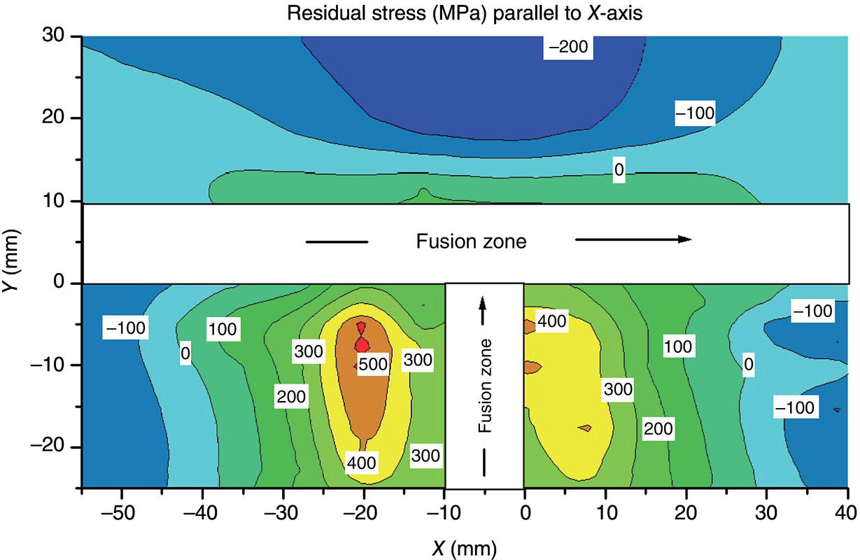
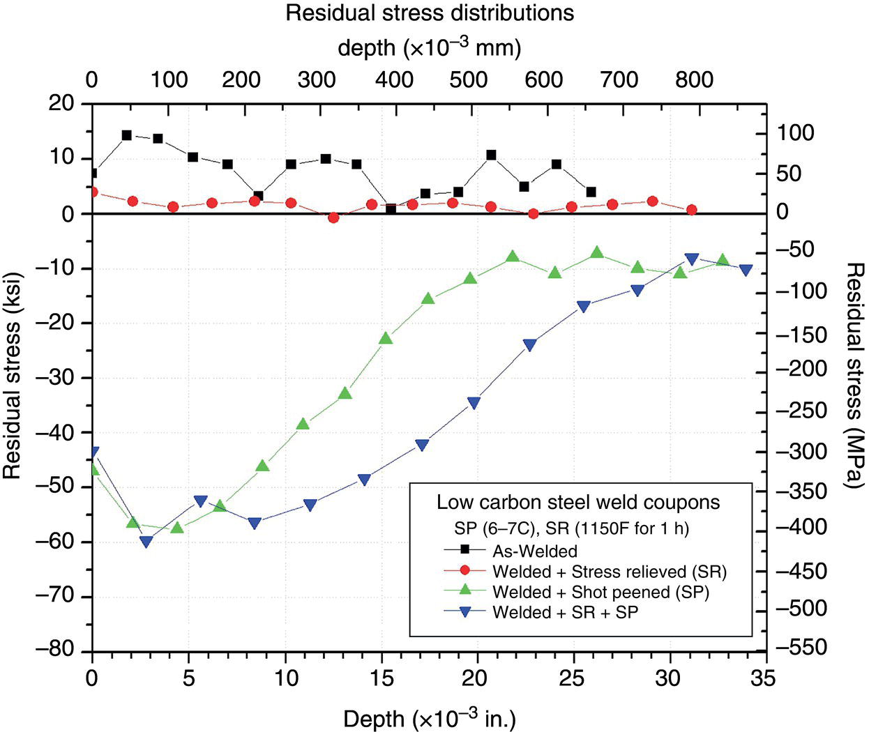
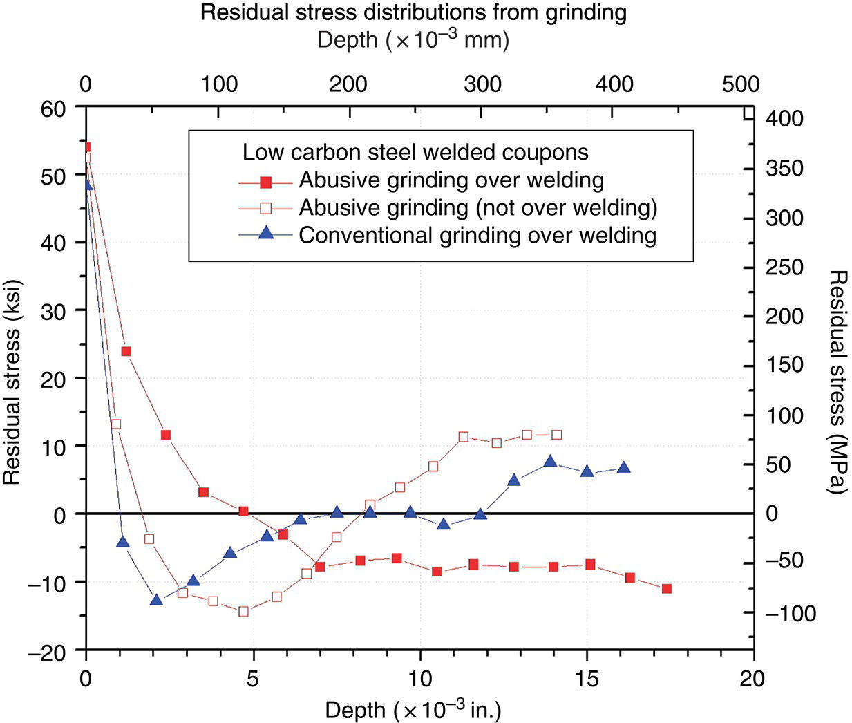
12.2 The Influence of Residual Stresses on Performance
12.2.1 Fatigue
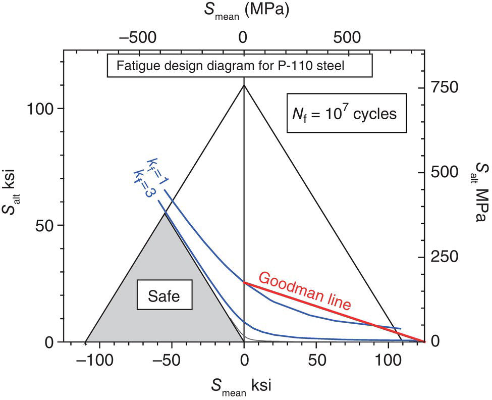
12.2.2 Stress Corrosion Cracking
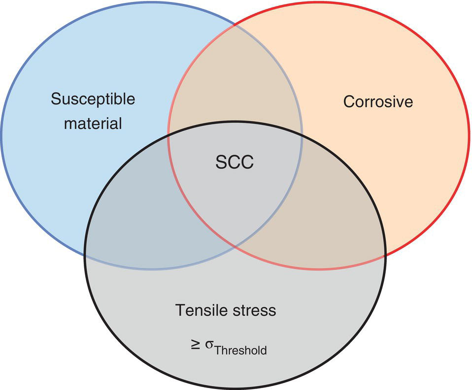
12.2.3 Corrosion Fatigue
12.2.4 Effects of Cold Working and Microscopic Residual Stresses
12.3 Residual Stress Measurement
12.3.1 Center Hole Drilling Method
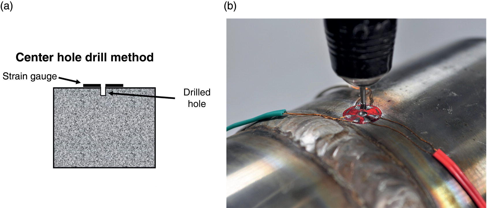
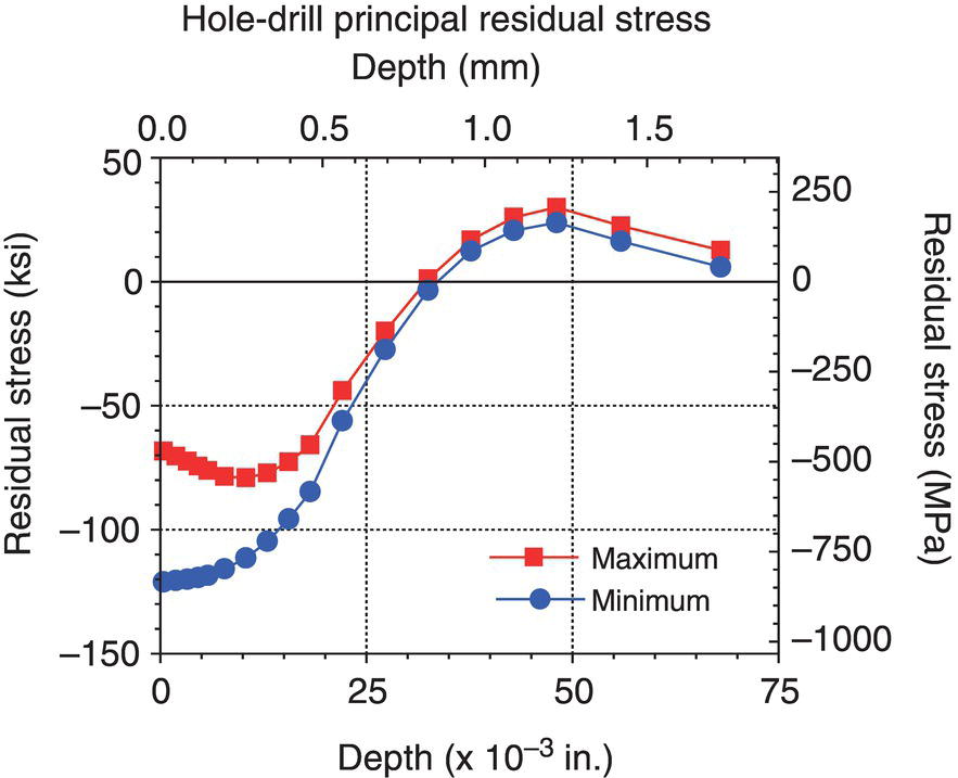
12.3.2 Ring Core Method
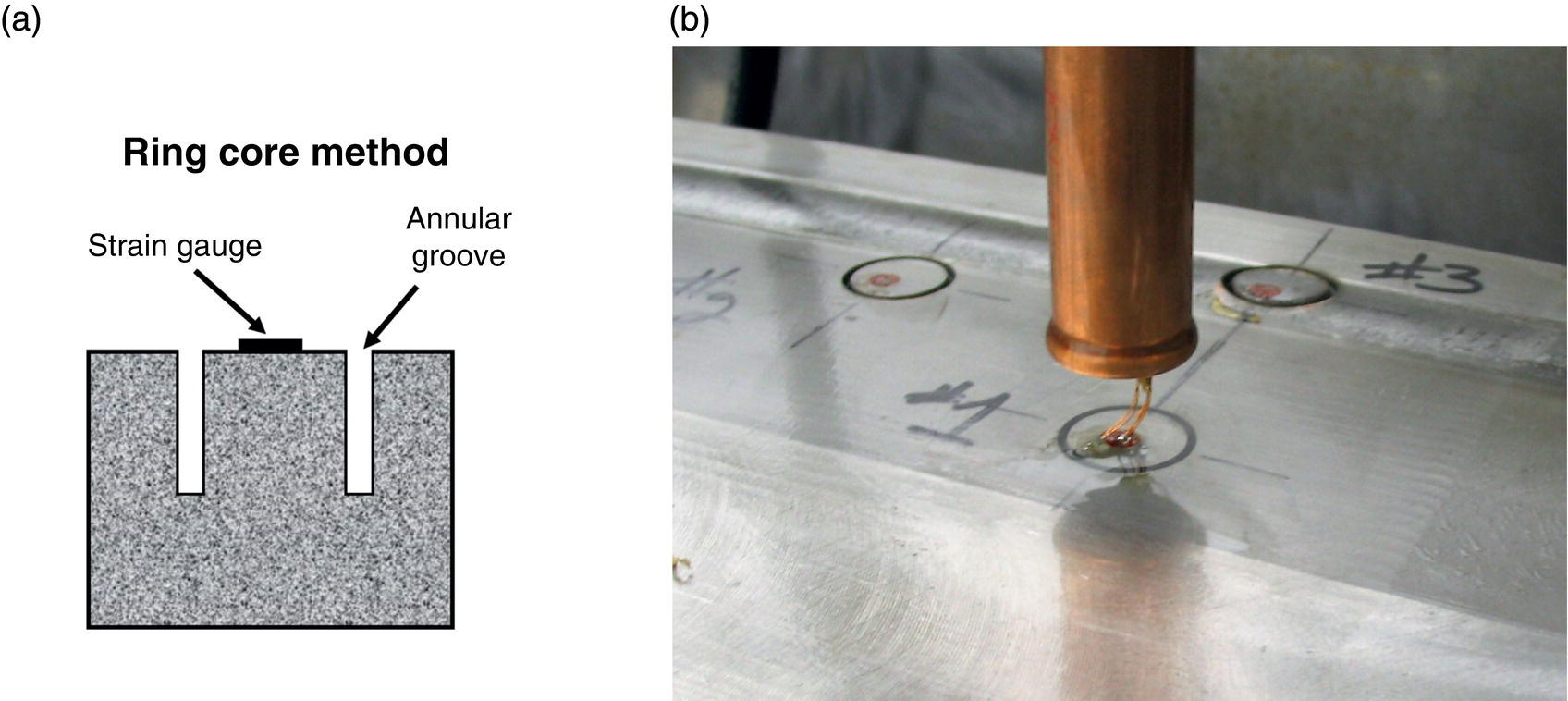
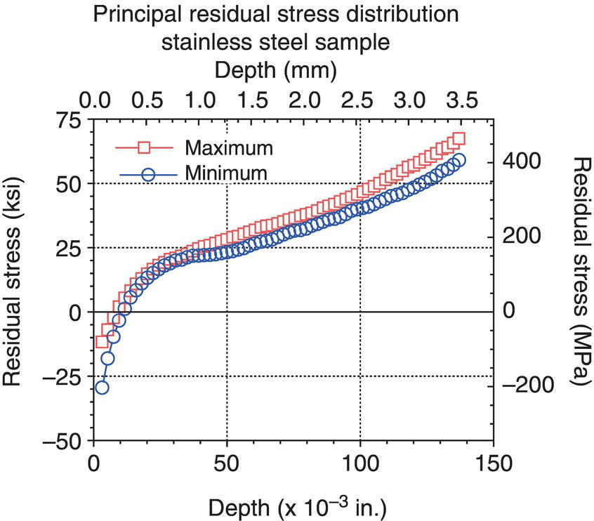
12.3.3 Slitting and Slotting Method
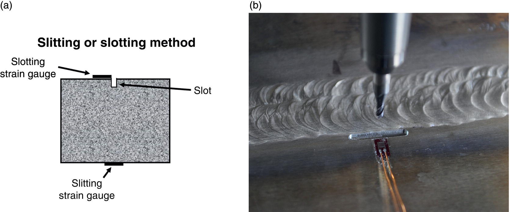
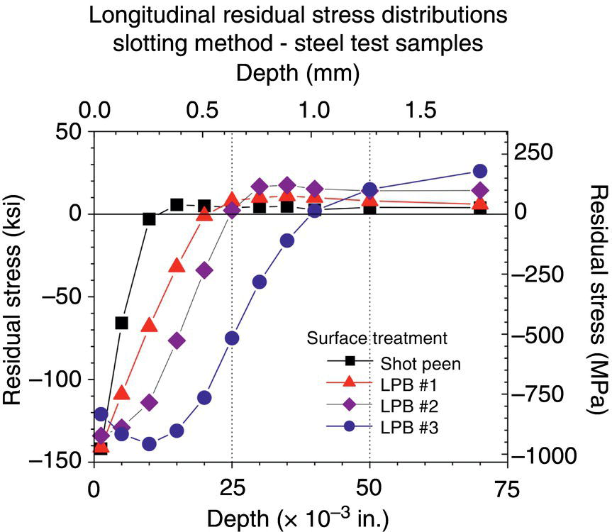
12.3.4 Deep Hole Drill Method
12.3.5 Diffraction Methods
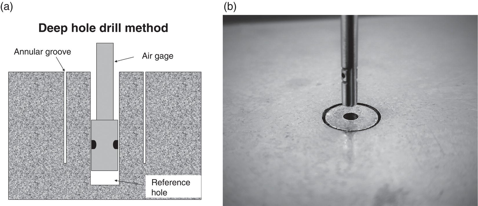
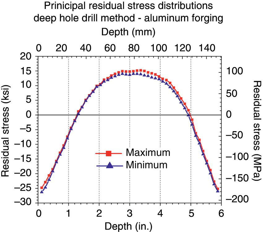
12.3.5.1 Principles of X-Ray Diffraction Stress Measurement

12.3.5.2 Plane Stress Elastic Model
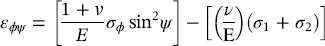
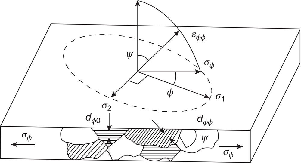
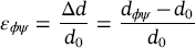
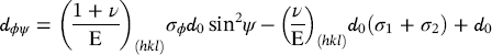

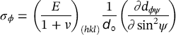
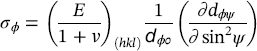
12.3.5.3 Sources of Error
12.3.6 Synchrotron X-Ray and Neutron Diffraction: Full Stress Tensor Determination
12.3.7 Magnetic Barkhausen Noise Method
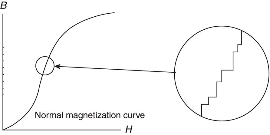
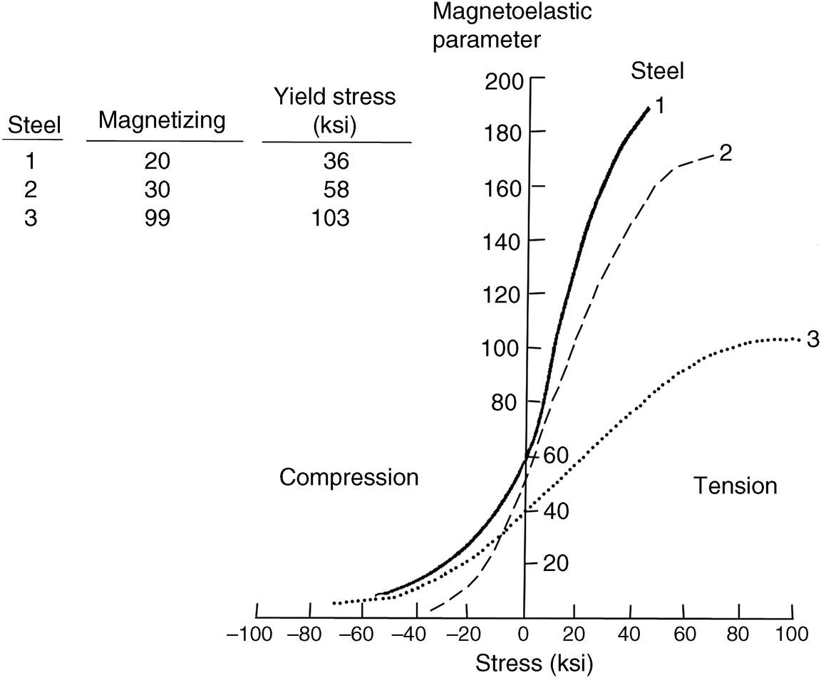
12.4 Control and Alteration of Residual Stresses
12.4.1 Shot Peening
12.4.2 Roller or Ball Burnishing and Low Plasticity Burnishing
12.4.3 Laser Shock Peening
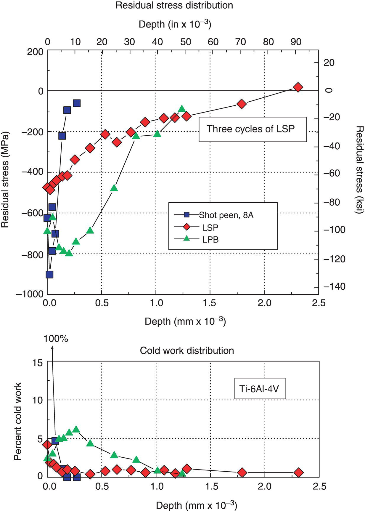
12.4.4 Thermal Stress Relief
12.5 Case Studies of the Effect of Residual Stress and Cold Work
12.5.1 Case Study 1: Restoration of the Fatigue Performance of Corrosion and Fretting Damaged 4340 Steel
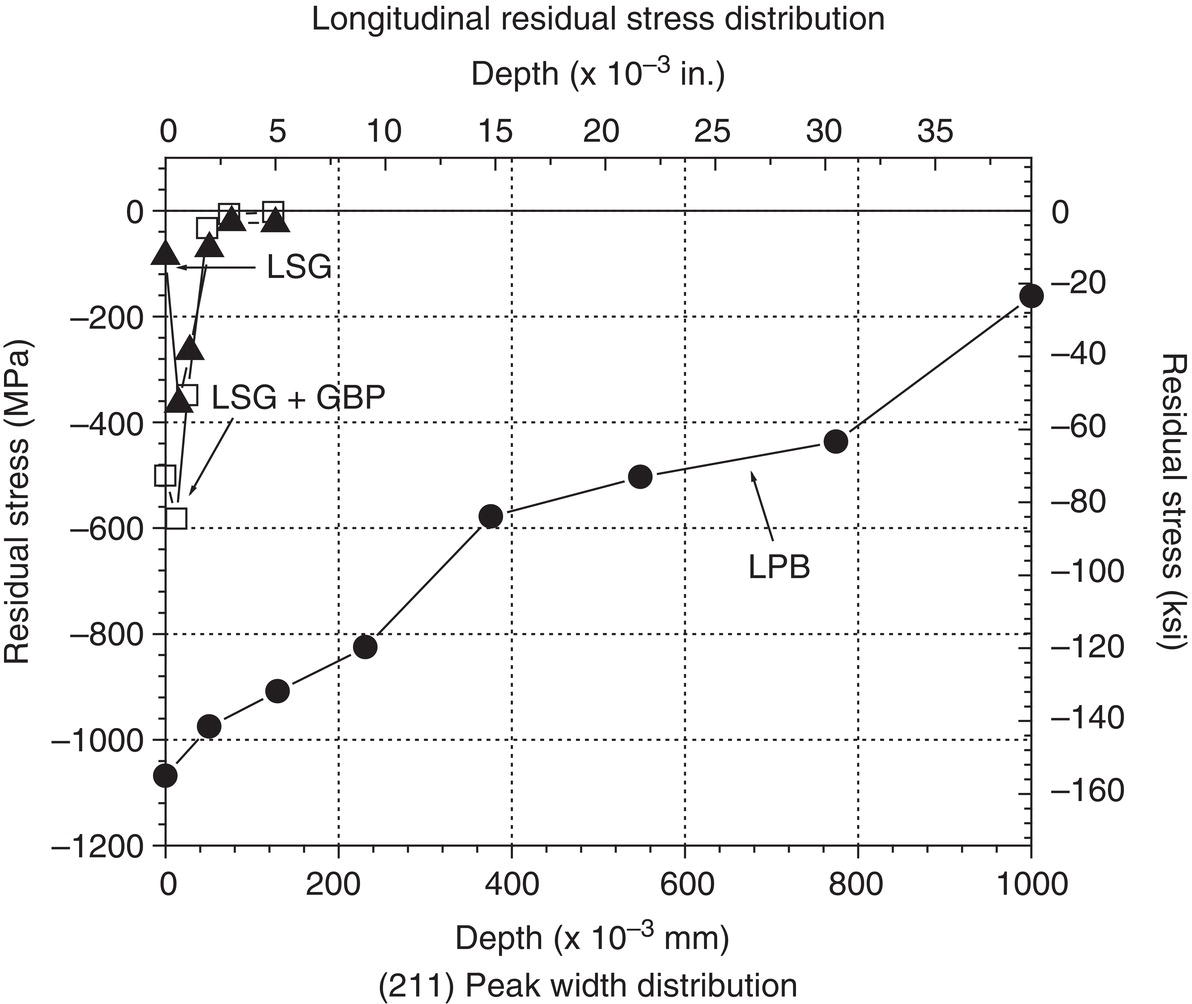
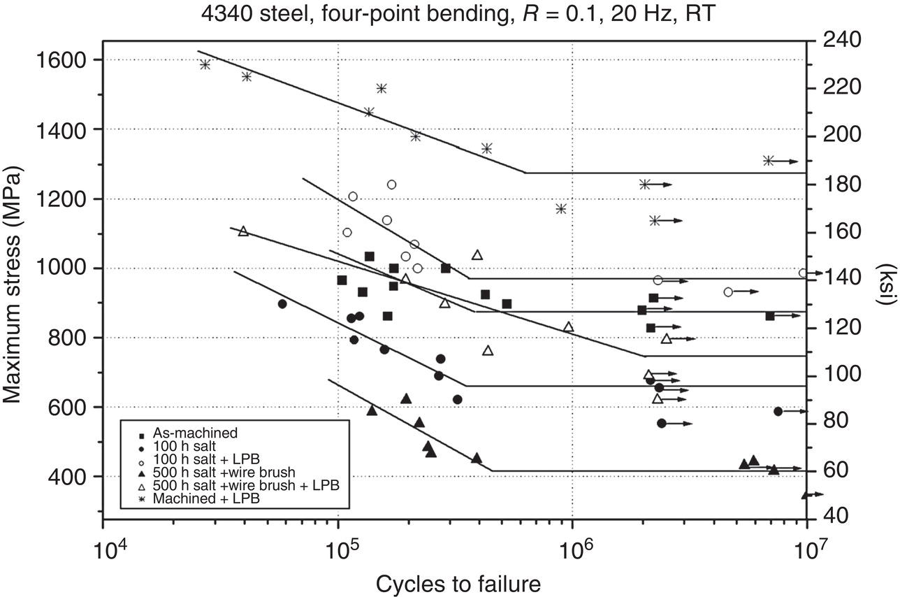
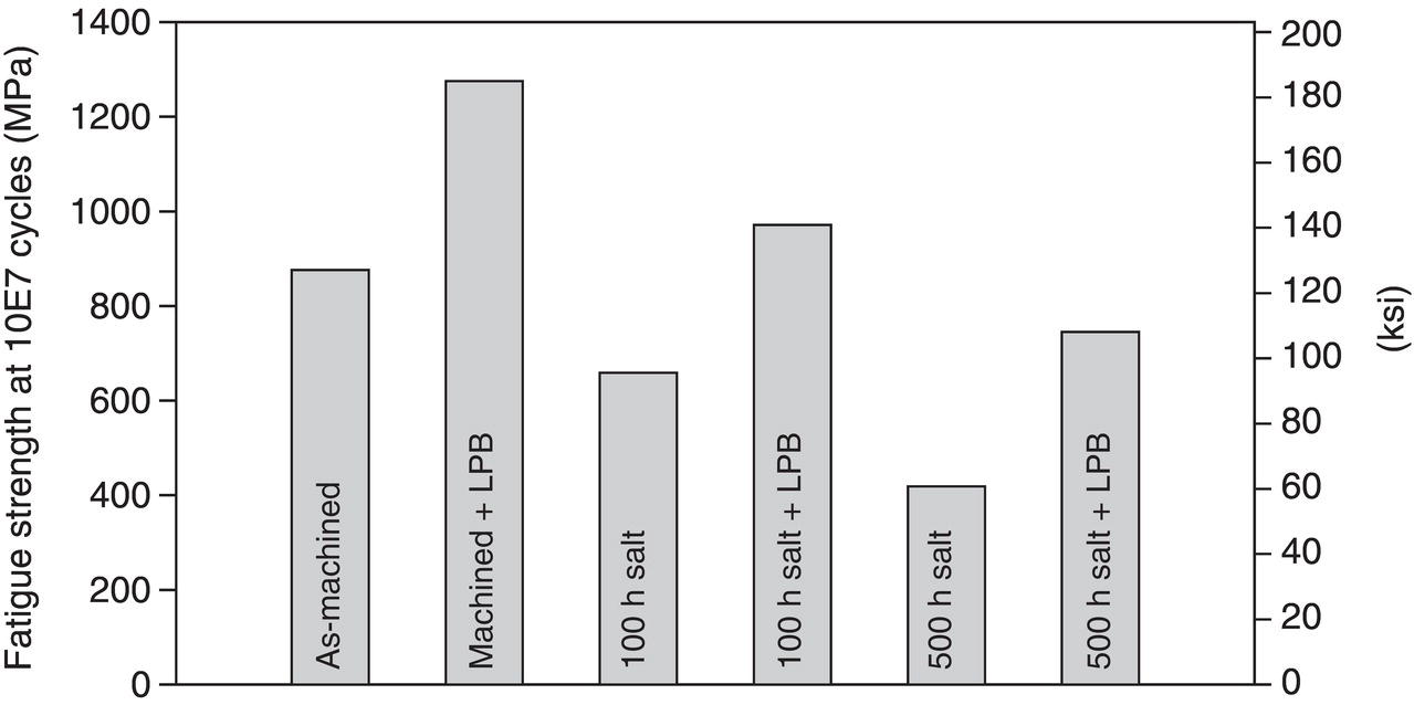
12.5.2 Case Study 2: Mitigating SCC in Stainless Steel Weldments [40]
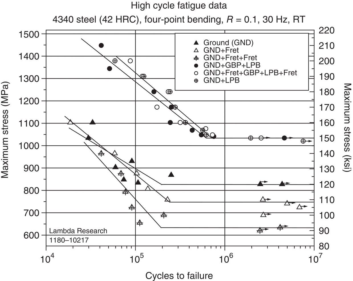
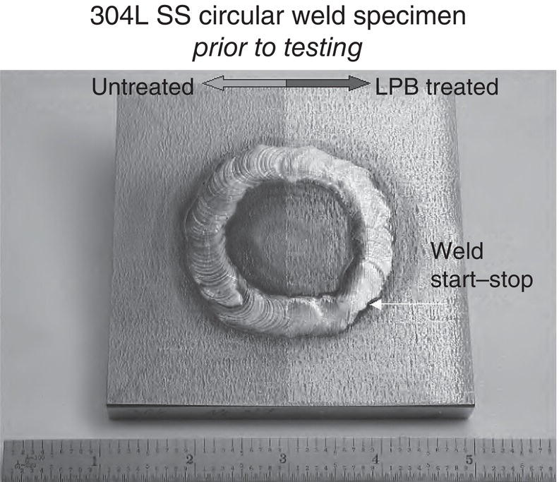
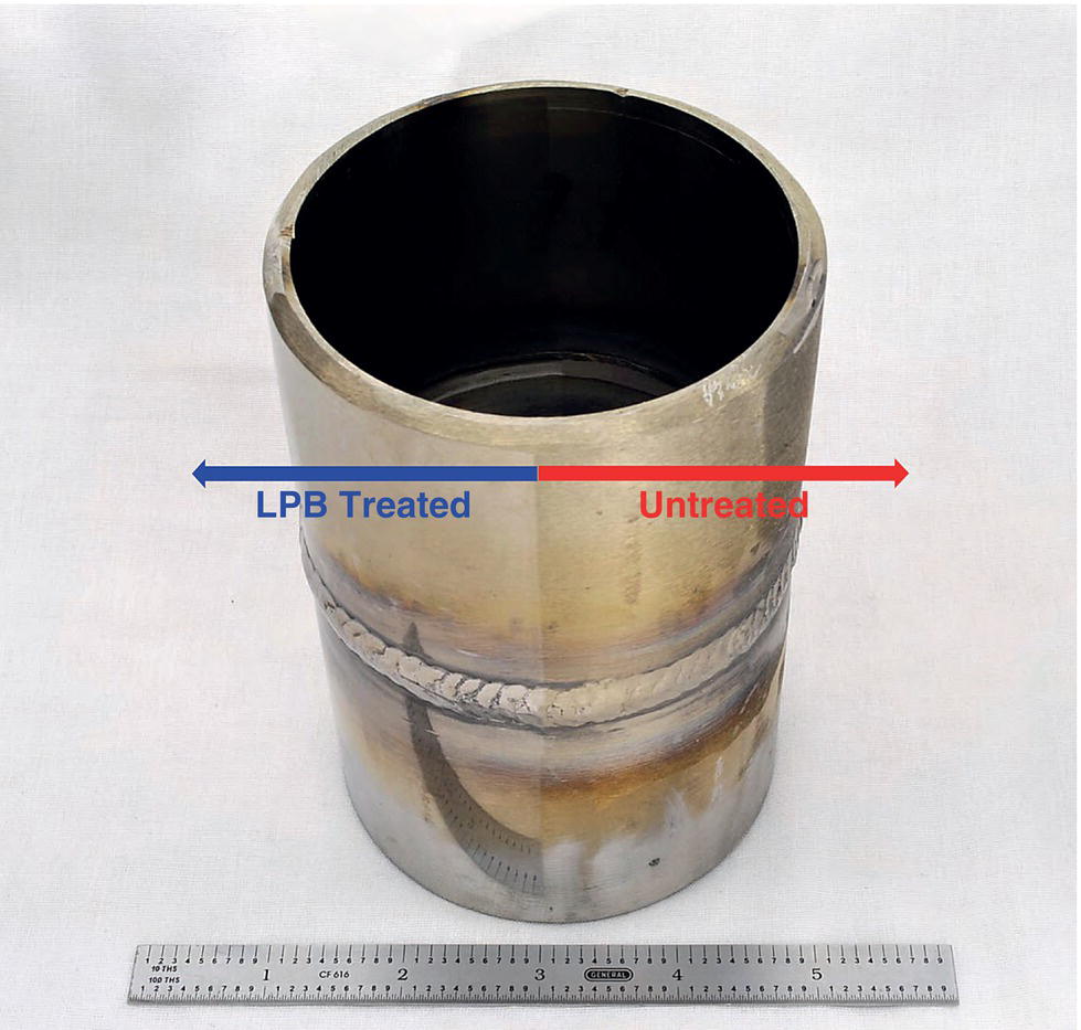
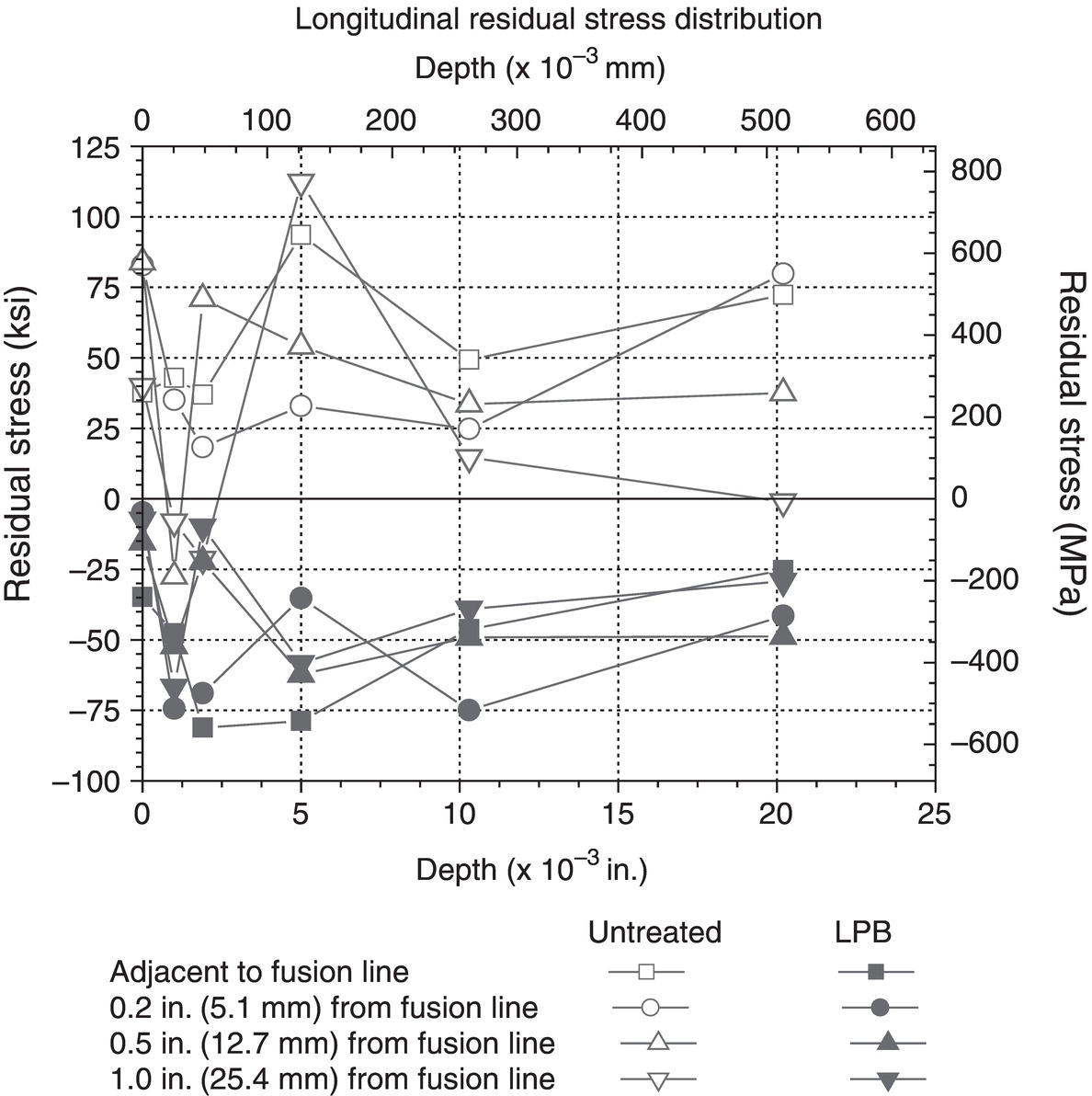
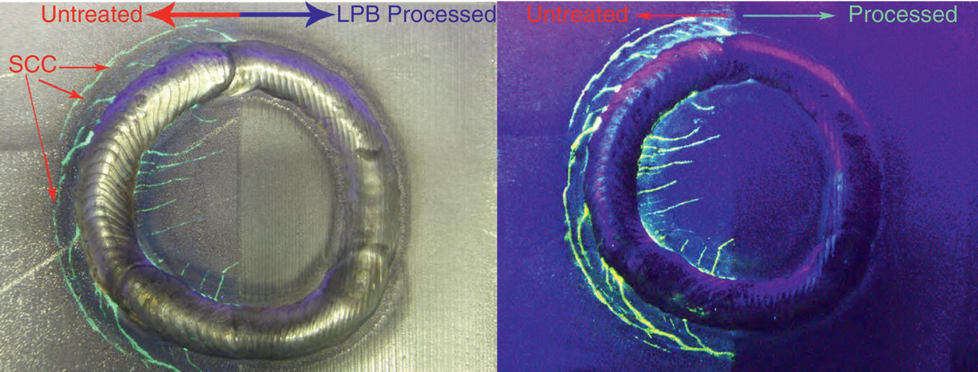
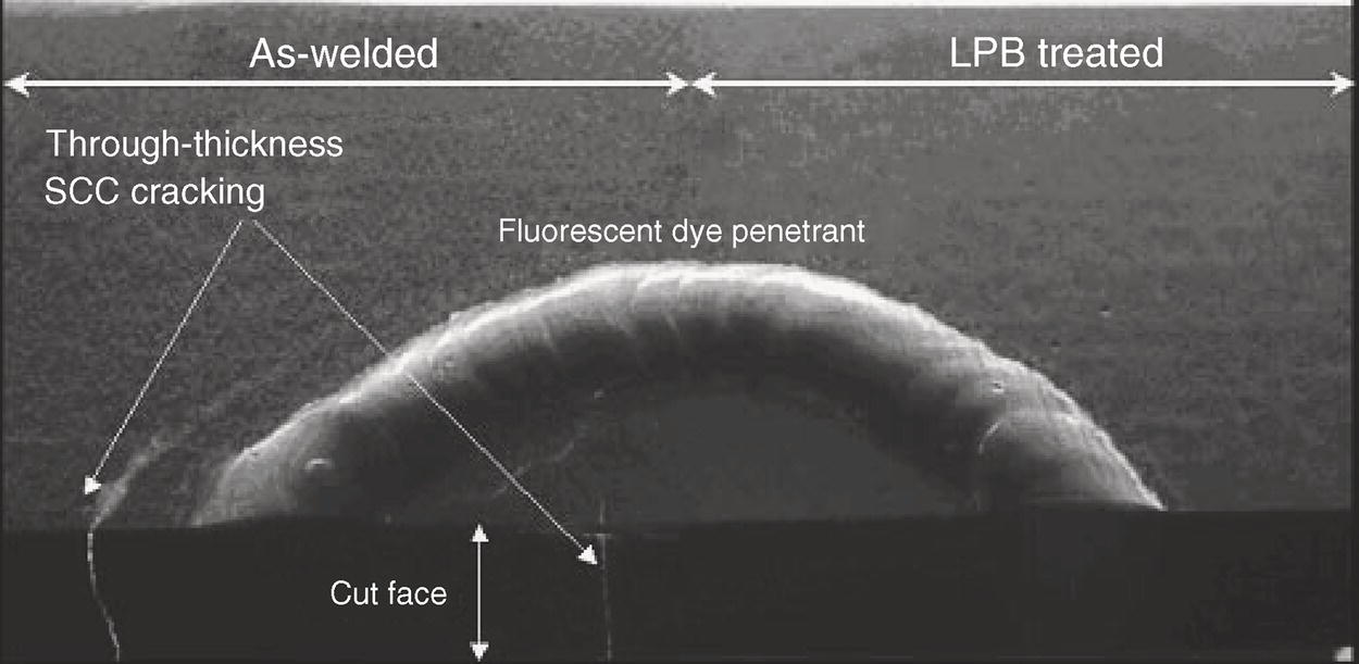
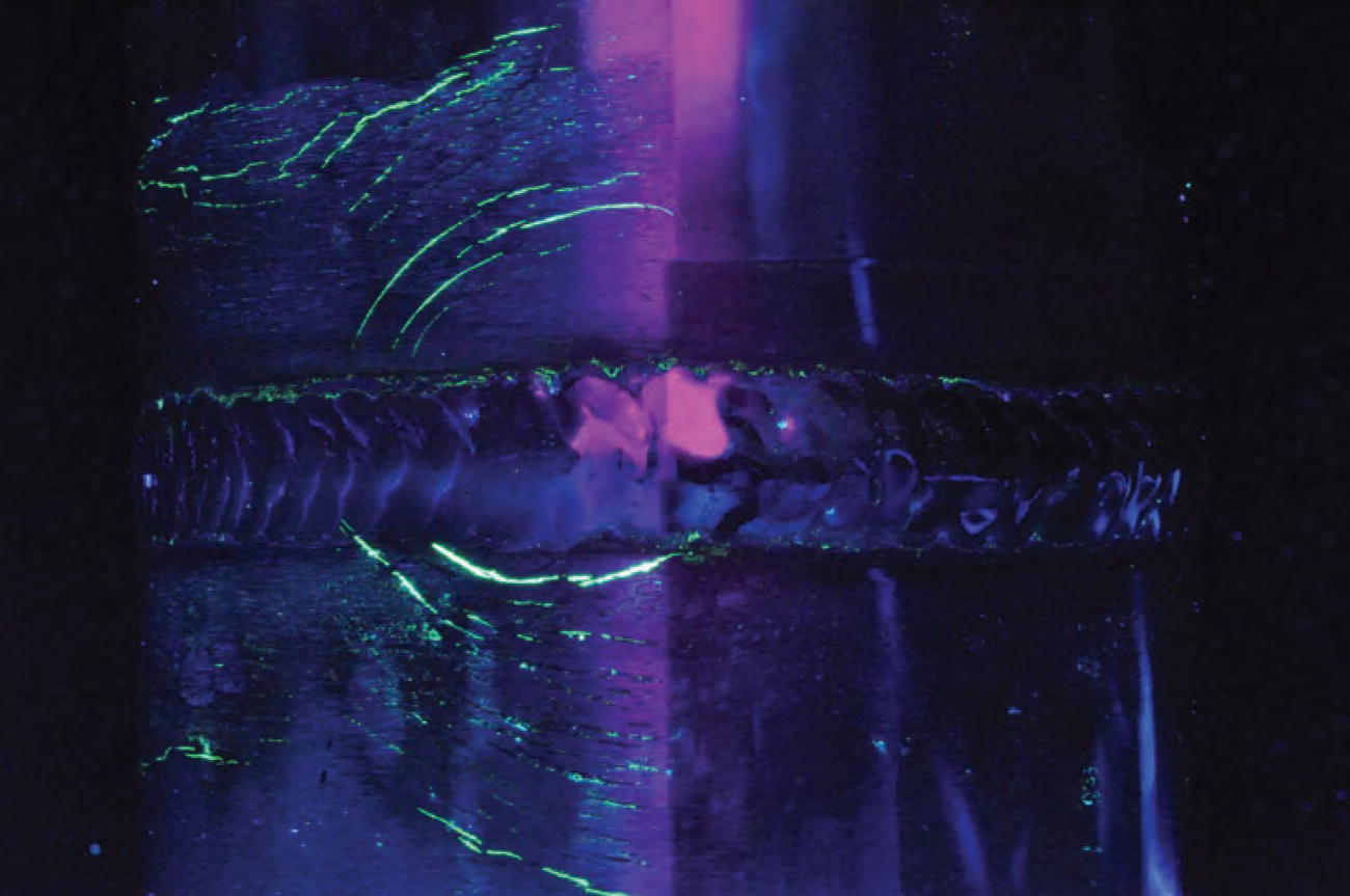
12.5.3 Case Study 3: Mitigation of Sulfide Stress Cracking in P110 Oil Field Couplings [41]
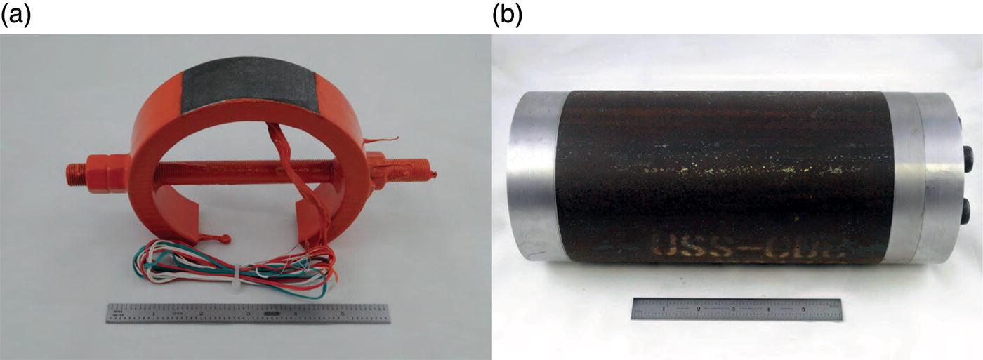
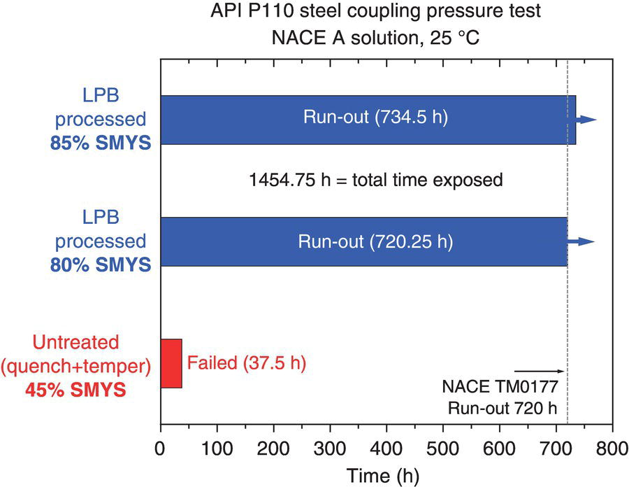
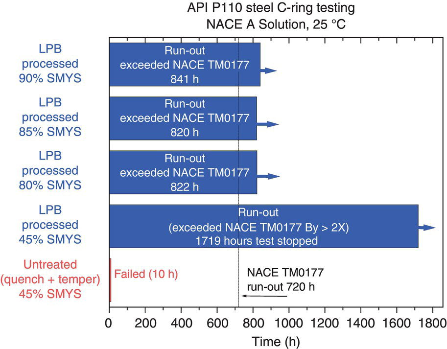
12.5.4 Case Study 4: Improving Corrosion Fatigue Performance and Damage Tolerance of 410 Stainless Steel [42]
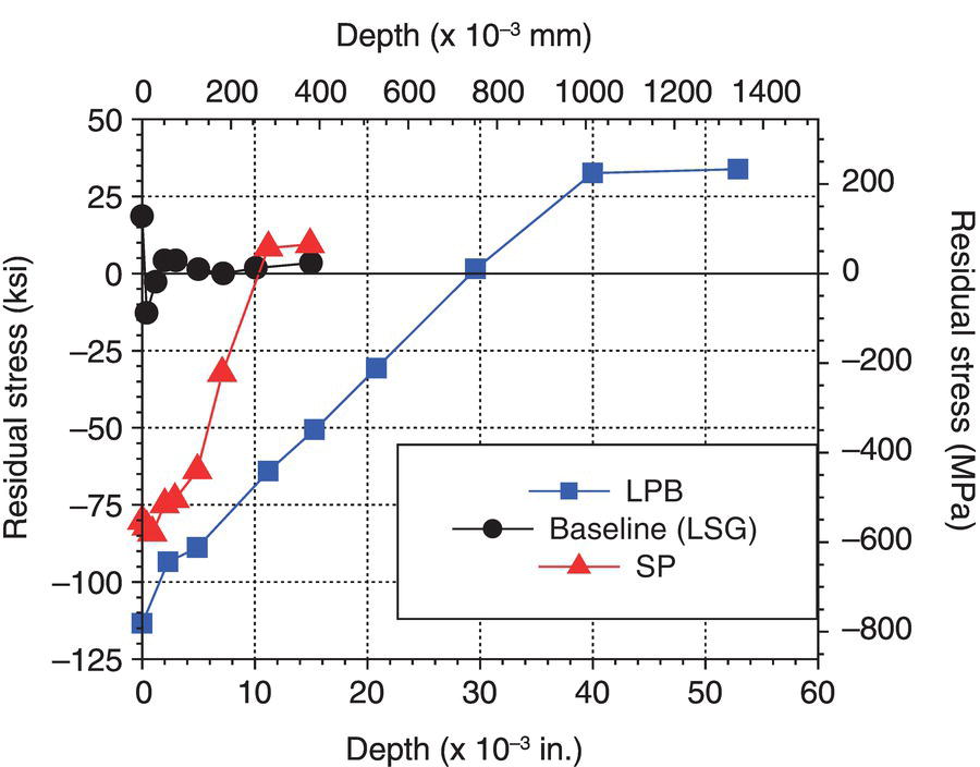
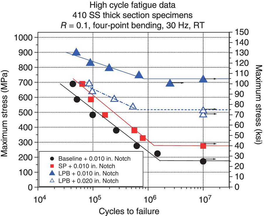
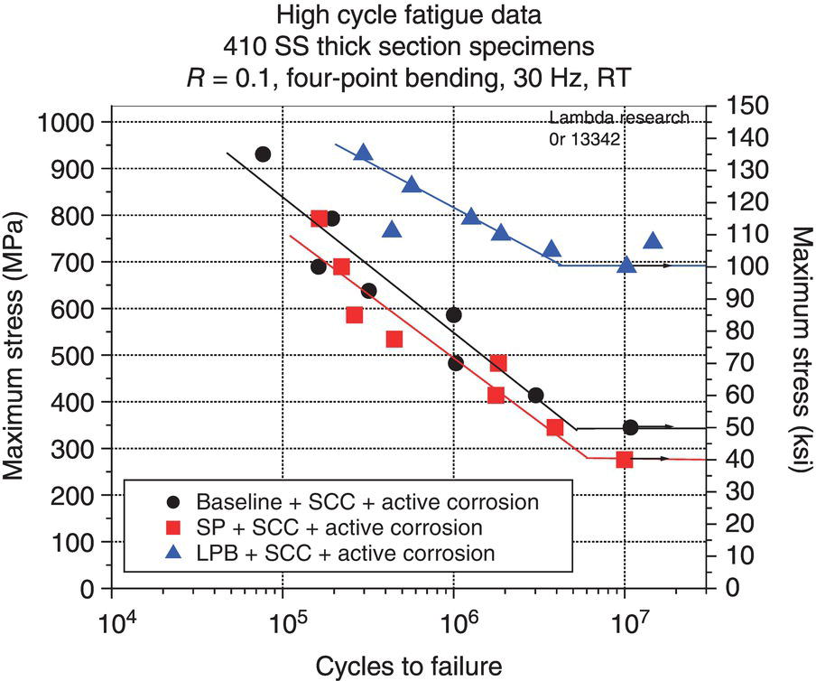
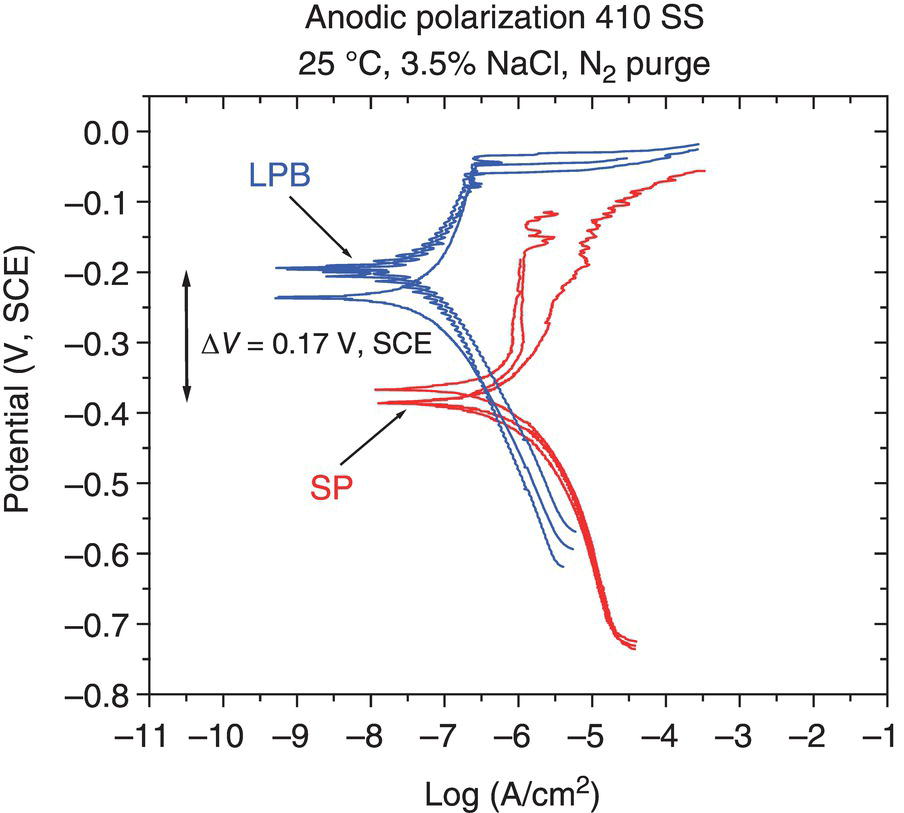
12.5.5 Case Study 5: Improving the Fatigue Performance of Downhole Tubular Components [43]
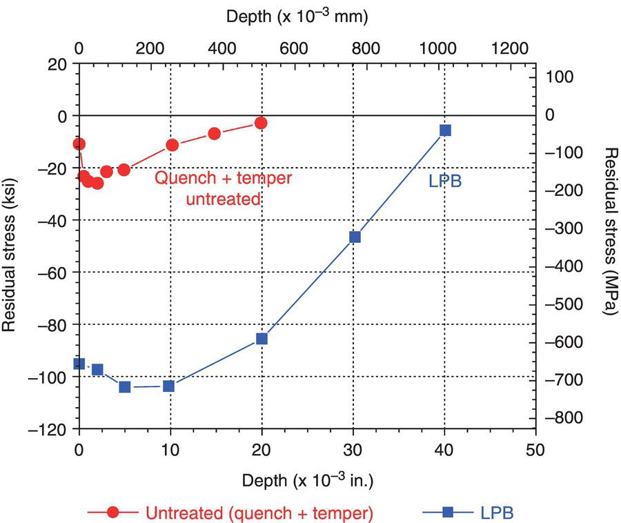
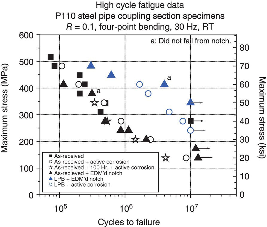

References
Note
Residual Stress in Pipelines
(12.1)
(12.2)
(12.3)
(12.4)
(12.5)
(12.6)