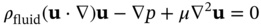
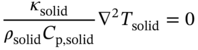
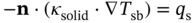
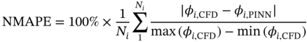
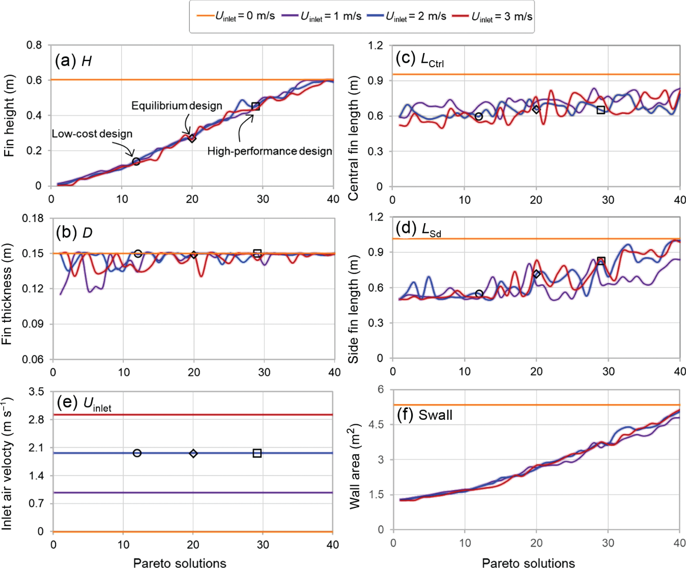
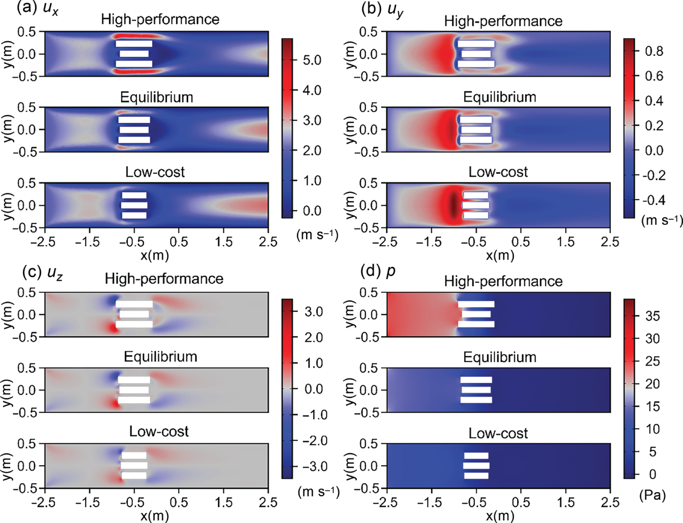
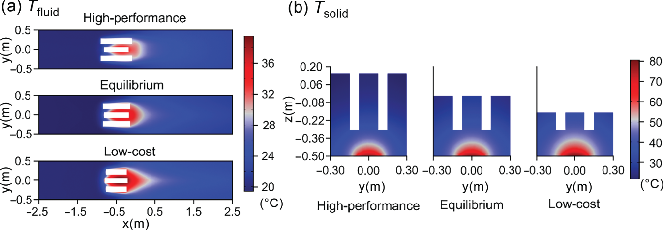
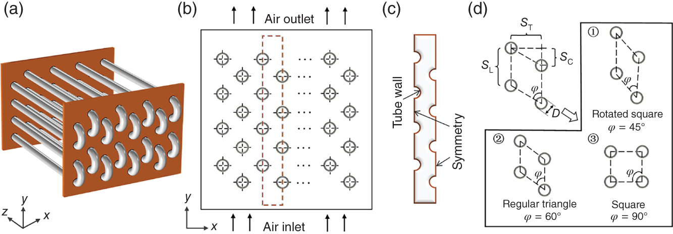
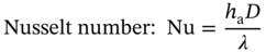
1Sun Yat-Sen University, School of Chemical Engineering and Technology, No. 135, Xingang Xi Road, Zhuhai, Guangdong 519082, China 2The Key Laboratory of Low-carbon Chemistry & Energy Conservation of Guangdong Province, Guangdong Engineering Center for Petrochemical Energy Conservation, 132 Waihuan East Road, University City, Panyu District, Guangzhou 510275, China 3Sun Yat-Sen University, School of Materials Science and Engineering, No. 135, Xingang Xi Road, Guangzhou 510275, China Designing high-performance and low-cost heat exchange systems for energy savings and emissions reduction has been a long-lasting challenge in electronic devices, power plants, and petrochemical processes [1–3]. To address this challenge, traditional practices typically rely on a trial-and-error or empirical procedure [4–6], where successive candidate solutions are generated through space-filling experimental designs over the combined space of the inputs (including geometric variable In contrast to intuition-based approaches, inverse design directly starts with the targeted functionality and sets it as an objective function to be optimized via partial differential equation (PDE)-constrained shape or topology optimization. When the geometry is represented by using the parameterized function of discrete geometric components, inverse design is known as shape optimization. On the other hand, when the geometry is parameterized by using a density function or level set so that the connectivity/structure/layout is arbitrary, inverse design is known as topology optimization [11, 12]. In this case, PDE-constrained inverse design can be performed via gradient-based optimization algorithms, where the gradient is obtained using adjoint methods that compute the gradient of the objective function with respect to all involved parameters. These methods are commonly based on numerical PDE solvers built into commercial CFD software, which tracks the interactions and spatial movement of each particle characterized by computationally expensive PDEs [13]. Moreover, data interface and transfer issues would lead to inefficient integration of numerical models with equation-oriented optimization frameworks since a large number of recourses to the PDE solver have to be executed before converging to the optimum. The time and memory costs further increase exponentially, which may cause a combinatorial explosion in the computation burden if no effective approach is applied. Figure 6.1 Traditional mesh-based numerical method for determining the optimal designs. In recent times, a prevalent approach to addressing the aforementioned computational burden has been the use of data-driven surrogate-based optimization. This is typically achieved by extensively studying shortcut models or detailed full-order models (FOMs) [14]. Shortcut models, employed to parameterize the geometry, consist of computationally inexpensive analytical or lumped parameter equations (rather than governing PDEs) with numerous ideal assumptions [15, 16]. These assumptions include perfect mixing, plug flow, and equilibrium behavior, among more. Consequently, it becomes advantageous for researchers to develop automated procedures that can effectively explore the design space by coupling with optimization algorithms such as mathematical programming [16, 17] and metaheuristic methods [18]. However, such approaches do not scale up well with the system’s size and would suffer from inaccurate and mismatch issues due to the insufficient description of the spatially distributed multiphysics phenomena inside a heat exchanger. By contrast, the FOM-based surrogate model can accurately capture the distributed phenomena. Neural networks, Kriging and radial basis functions, and specialized regression models are often employed in a supervised-learning paradigm to learn the nonlinear mapping from arbitrary designs to their associated objectives, i.e. neural networks are regarded as surrogate models of the original FOMs to accelerate the design and optimization [17, 18]. Nevertheless, it often requires a large number of datasets to form high-fidelity surrogate models, particularly for coping with complex varying geometry problems, where the generation of such datasets via conventional PDE solvers could become prohibitively expensive. As a result, the benefit of data-driven surrogate-based optimization must be weighed against model accuracy and time cost to resolve them, which is a major driver and could impede the development of better designs for heat exchange systems. With the explosive growth of computing and data resources, deep learning has shown promise for simulation, modeling, and optimization due to its capability of handling strong nonlinearity and high dimensionality issues. Recently, the physics-informed neural network (PINN) developed by Karniadakis et al. and coworkers [11, 12, 19, 20] has opened up a deep learning, mesh-free route to solve governing PDEs by mathematically encoding the underlying physics (e.g. conservation laws, transfer laws, and kinetic equations) into the loss function of the neural network. The governing PDEs can take various forms, such as integer-order PDEs [21], integrodifferential equations [22], fractional or stochastic PDEs [23–25], and so on. One of the notable strengths of PINN is its ability to efficiently take the derivatives of a neural network by applying chain rules for differentiating the compositions of PDEs using automatic differentiation [26]. PINN has been successfully applied to diverse areas such as fluid mechanics [27–29], medical diagnosis [30–32], heat transfer analysis [33–35], and materials science [36–38]. Moreover, due to its capability of learning physics equations in rich representation as well as the use of automatic differentiation that removes the need for mesh generation, physics-informed learning is well-placed to become a natural bridge that integrates the numerical model with the optimization procedure for accelerating the discovery of optimal geometry designs. Despite the recent success and promising prospects of PINN, it has been found that this approach is currently limited to tasks characterized by relatively simple and well-defined physics [10, 20]. Existing research on PINN generally aims to construct a high-fidelity surrogate model of the investigated system using a single deep neural network to control all variables and derivatives in the PDEs. It often struggles to accurately penalize residuals or even fails to train, particularly when tackling multiphysics and multiscale problems with high-frequency functions [10]. For example, heat sink systems typically involve a conjugate heat transfer process [39–41], which is a combination of heat transfer in fluids and heat transfer in solids. As a result, the involved physical variables or parameters (such as velocity, pressure, and temperature) have distinct meanings and may extend over several orders of magnitude in on spatial scales. However, most studies have applied encoding to the parametric inputs using a single variable or parameter in PDEs, without focusing on boundary conditions or geometric dimensions, as well as multivariable parameterization issues. When applying the stand PINN method to approximate this process, the trained neural networks and constructed surrogate models are not robust and stable enough, which are not conducive to subsequent tasks such as real-time prediction and design optimization. Therefore, the extension of the standard PINN to accomplish the parameterized system representation task is technically challenging and requires significant improvements in the structure and algorithm of the neural network for better accuracy, faster training, and improved generalization. This chapter aims to not only use the PINN for modeling heat exchange systems with complex geometries but also propose an inverse design method that seamlessly combines the constructed surrogate model with multi-objective optimization and decision-making algorithms. For simulating the involved heat and mass transfer processes, specialized neural network structures are developed to decompose the standard PINN model into multiple interconnected subnetworks with identical architecture, which were functionally designed to approximate the latent solutions of the governing PDEs. In addition, the developed PINN applies the input encoding to the geometric and operating inputs in a fully decoupled setting and then concatenates them together in surrogate modeling. This surrogate model, combined with multi-objective optimization and decision-making methods, not only delivers the Pareto-optimal solutions directly but also allows real-time visualization of the distributions of the monitored state variables for better physical inspection. Results are presented for two illustrative examples: (i) In the first example, we demonstrate the proposed method’s ability to describe the underlying behaviors of conjugate heat transfer inside the heat sink system. (ii) In the second example, we further leverage the capabilities of space decomposition, physics-informed deep learning, and transfer learning to accelerate the multi-objective stochastic optimization of a tubular air cooler system. This chapter is derived from the work of He and coworkers [42, 43]. This section begins by providing a brief introduction to the inverse design problem. Subsequently, the standard PINN method is presented, along with the PINN-based optimization and decision-making methods utilized to address this problem. Given a steady-state heat exchanger, the governing PDEs can be represented by a generic form defined on a bounded domain Ω ⊂ ℝ3 with suitable boundary conditions where where x = [u, p, T]T, xD, and xN are the coordinates of ∂DΩ and ∂NΩ, ∂Ω = ∂DΩ ∪ ∂NΩ, ∂DΩ ∩ ∂NΩ = ∅; n is the unit normal vector outward to the boundary at xN. Here, the initial condition can be simply treated as a special type of Dirichlet boundary condition on the domain [45]. The latent solution of the PDEs, μ(x) = [μ1(x),…, μn(x)] ∈ ℝn, is determined by the independent variable set λ = [λ(1), λ(2)], which is our quantity of interest for the inverse design problem [11]. Here, it is noted that λ includes design variable λ(1) and control variable λ(2), which describe the specific shapes/structures to be manufactured and the corresponding operating conditions to be maintained for realizing an optimal design, respectively. To address this complex problem, traditional intuition-based approaches have to indirectly convert it into a large number of forward-design problems via experimental design or even brute-force search. This is done until a feasible solution is found by evaluating the outputs of all objective values of interest. As presented in the Section 6.2.1.1, we utilize the advancements of PINN for inverse design optimization due to its natural capability of embedding physical models, as well as the use of automatic differentiation that removes the need for mesh generation. In particular, a deep neural network μnet is developed as a parametric surrogate model of the solution μ, where λ = [λ(1), λ(2)] satisfies all the equality constraints enforced by the governing PDEs and the boundary conditions. With the aid of this surrogate model, we can directly search for the best independent variable set λ* by minimizing objective functions of interest, Θ = [Θ1, …, Θm]. Besides, a set of equality/inequality constraints that stem from the multi-objective problems of the system, as well as the thermal and hydraulic requirements, are also incorporated in the inverse design. In all, the multi-objective inverse design problem can be formulated by where h denotes the additional equality or inequality constraints. The PINN algorithm can parameterize a physical model by applying the input encoding to the temporal/spatial and parametric inputs and then concatenating these inputs together. It often uses a conventional feed-forward fullyconnected architecture, where a deep neural network represented by μnet(x, λ; θ) is constructed as a surrogate of the solution μ. As shown in Figure 6.2, μnet(x, λ; θ) takes the spatial coordinate x = [x, y, z] and parametric variables λ = [λ1, λ2,… λn] as the input and outputs a vector αL (i.e. u, p, T) that has the same dimension as μ. The training of the PINN aims to obtain the set of best parameters θ* = [w*, b*] by minimizing loss terms (ℒf and ℒb) such that the neural network can approximate the solution of the original PDEs. Figure 6.2 Schematic of the standard PINN algorithm for parametric surrogate modeling. Source: [19]/with permission of Elsevier. The derivative terms (i.e. ∇and ∇2) are handled via automatic differentiation. a = σ[·] denotes a nonlinear activation function. where w and b are weight matrices and bias vectors of the neural network, respectively, which will be tuned at the training stage. In order to train PINN, the derivative terms of μnet with respect to its inputs are computed by applying the chain rule for differentiating compositions of the functions using automatic differentiation. Next, the neural network μnet is restricted to the training points where and ωf and ωb are the weights that balance the interplay between the two loss terms ℒf and ℒb; || ||2 denotes the L2 norm of residuals. Two mutually independent sets, To improve the training performance, the loss function of PINN can take the form of Monte Carlo integration approximation [46] since it can ensure the consistency of the loss per volume across the domain. Additionally, it is worth noting that the weighting coefficient in the loss function plays a pivotal role in enhancing the accuracy of PINN, which can be user-defined or tuned automatically. It is often defined as a fixed value that does not vary with the spatial position of the sampled points in the flow field or on the boundary. Nevertheless, the gradient profile at several positions of the flow field varies greatly (e.g. sampled points nearby the sharp corners or discontinuous areas), which makes a fixed weighting coefficient unreasonable. Here, the signed distance function (SDF) [47] is introduced in the loss function to weigh the loss terms, by which each weighting coefficient can be a function of the spatially distributed points in the spatial domain. The SDF is defined as follows [48]: where where d(x) represents the minimum distance of a given point from ∂Ω. According to this definition, the absolute value of SDF often decreases close to zero near the boundary of the domain, where sharp gradients occur. Hence, weighting by the SDF tends to reduce the impact of sharp gradients on the convergence, which contributes to speeding up the learning rate and sometimes also improves prediction accuracy. Overall, by combining the SDF and Monte Carlo integration approximation, the combined loss function for training the parameters of each subnetwork is as follows: Another similar training strategy, namely integral continuity plane [49], can be used for enforcing the conservation constraints (e.g. mass, volume, and energy equations) of a given control volume in the domain. For example, we can specify that the volumetric flow of coolant passing through the heat exchanger system must be equal to that entering the system in the flow channel, as listed in Eq. (6.14). This conservation constraint helps to accelerate the solution of the continuity PDEs. Similarly, the heat flux of coolant entering the flow channel, along with the heat flux generated by the working heat source, must be equal to that leaving the channel. Such heat flux conservation is also expressed in an integral form, as given by Eq. (6.15). where Ainlet and Asource are the areas of the channel inlet plane and heat source surface, respectively. The training hyperparameters of the neural network, e.g. network sizes, learning rates, optimizers, initializations, and regularizations, also need to be fine-tuned to achieve a good level of accuracy. More details of the training strategy can be found in Refs [45, 49]. Finally, it should be pointed out that the standard PINN uses a single neural network to construct a surrogate of the solution μnet. While this approach has demonstrated promising results in certain applications, its limitations become apparent in more complex multiphysics and multiscale tasks that involve high-dimensional and intricate geometric domains. For example, heat sink systems typically involve a convective heat transfer process, which entails a two-way coupling of fluid flow and heat transfer. In practice, however, it is challenging to precisely penalize the residuals in training the neural network of this process in a fully coupled setting. This is because the terms in the combined loss function have distinct physical meanings, such as velocity, pressure, and temperature, and may span several orders of magnitude in spatial scales, making the training process less robust and stable. In the field of multi-objective optimization, previous studies [50–52] have often relied on evolutionary methods, which mainly include decomposition-based and Pareto-based approaches. The former typically uses a scalarizing function to aggregate all the objectives into a single scalar objective function or retain only one objective while enforcing the others as constraints. A major issue with this approach resides in the extensive knowledge of the problem structure, and not all scalarizing functions can guarantee that all Pareto-optimal solutions are obtainable [53]. The latter can make full use of the Pareto-dominance relations to induce partial ordering in the objective space. It provides a more convenient way to obtain a set of solutions toward the Pareto front and covers the entire Pareto front. One of the most widely used algorithms is the Non-dominated Sorting Genetic Algorithm II (NSGA-II) [54], which is employed in the present study. It is noted that the alternative solutions of the multi-objective optimization on the Pareto-optimal front have the same worthiness based on optimization objectives in the absence of additional preference information, which entails a need to identify the most preferred solution for decision-makers in practice. To this end, a classic decision-making method, namely technique for order preference by similarity to ideal solution (TOPSIS) [55, 56], is subsequently used to identify the most preferred solution closest to the positive-ideal solution and furthest away from the negative-ideal solution as the compromise scheme. Assuming the number of alternative solutions is M, the procedure of the TOPSIS method can be divided into the following steps: where where ωn is the weighting factor of the nth criterion, ∑ωn = 1. A 3D finned heat sink system with forced air cooling [57] is used as a motivating example in this chapter. As shown in Figure 6.3, the base plate with a built-in chip is placed on the bottom center of a rectangular channel, which is directly in contact with the flat base of the heat sink system through thermal conductive adhesive. In this way, we can consider that almost all heat flux generated by the hot chip can be transferred to the fins on the flat base. Meanwhile, the coolant medium (air) introduced from the channel inlet flows to the surface of the fins, which aims to promptly take away the transferred heat and prevent the junction temperature of the chip from reaching the threshold value. In summary, the heat sink system involves a 3D, steady-state conjugate heat transfer process. Figure 6.3 A schematic view of the geometry of the finned heat sink system. (a) 3D view, (b) left view, and (c) bottom view. In 3D modeling, the center of the channel is used as the origin of the Cartesian coordinate system. Source: [42]/with permission of Elsevier. The heat sink system involves a 3D, steady-state conjugate heat transfer process, which combines heat transfer in fluids with heat transfer in solids [58]. In fluids, heat convection dominates the heat transfer process. We assume that fluid passes through the system subject to incompressible and laminar flows, the governing continuity and Navier–Stokes equations are as follows [59]: where u = [ux, uy, uz] denotes the fluid velocity vector; ∇ denotes the Hamiltonian operator; p, ρfluid, and μ denote the static pressure, density, and dynamic viscosity of the fluid, respectively. Here, it is assumed that the thermophysical properties of the fluid and solid, as listed in Table 6.1, are constant and insensitive to temperature change in the flow field. Table 6.1 Thermophysical properties of fluid and solid. The occurrence of fluid heat transfer is based on the premise of fluid motion. Thereby, without internal heat sources, the governing equation of fluid heat transfer is given by where Tfluid, Cp,fluid, and κfluid are the temperature, specific heat, and thermal conductivity of the fluid. The first and second terms act as the convection term and diffusion term, which describe the thermal convection and heat conduction of fluid, respectively. While heat conduction plays a major role in solids, the temperature distribution can be directly determined by solving Laplace’s equation. where Tsolid, Cp,solid, and κsolid are the temperature, specific heat, and thermal conductivity of the solid, respectively. An essential condition for solving the aforementioned conjugate heat transfer problem is to provide well-defined boundary and initial conditions as model constraints, especially at the fluid–solid interface. First, for simulating the fluid flow process, a non-slip velocity condition (u = 0) is applied to both the channel wall and the fluid–solid interface. The initial air velocity at the channel inlet is known (ux = Uinlet, uy = 0, uz = 0), while the air pressure at the channel outlet is set to zero. For simulating the heat transfer process, the channel wall is modeled using an adiabatic condition (n·(κfluid·∇Tfluid) = 0) with a known temperature at the channel inlet (Tfluid = Tinlet). It is assumed that the hot heat source could create an even heat flow at the bottom of the flat base. With this assumption, a constant heat flux qs can be specified as a thermal boundary constraint for the heat sink model, as given by where ∇Tsb denotes the temperature gradient at the bottom of the flat base; n denotes the unit normal vector outward to the surface. Herein, to guarantee the continuity of heat flux and temperature at the fluid–solid interface, the following constraints are enforced on boundary conditions [60]: where the subscripts sw and fw denote the solid wall and fluid wall at the fluid–solid interface, respectively. The heat sink system generally aims at cost-effectively cooling down the running heat source to prevent thermal shutdown by exchanging sensible heat with air flowing through the surface of this system. Based on this premise, the first objective of interest is termed the mean surface temperature of the heat source (Tmean), which is often used as a key indicator to measure the cooling capacity of a given heat sink system. In addition, decision-makers are concerned about the operating cost of achieving a higher cooling capacity. For example, using complex fins with a larger heat exchange area would help to reduce the working temperature of the heat source, but it also incurs an additional pressure drop (Δp) in the airflow. In this case, increased power consumption by the intake fan is required proportionally. These two conflicting objectives can be calculated through the solid heat transfer network and fluid flow network, combined with the Monte Carlo integral approximation, as given by. where Aout denotes the cross-sectional area at the outlet of the channel. The peak surface temperature of the heat source (Tpeak) must be lower than the maximum allowable junction temperature (Tmax) to ensure the safety and reliability of the system [61]. A bi-objective optimization model is formulated to minimize the mean surface temperature and the pressure drop of the system, as given by: where Eqs. (6.29)–(6.31) are embedded as a surrogate model to predict the temperature and pressure drop. The superscripts lb and ub are the lower and upper bounds for the decision variables of interest for the present study, as listed in Table 6.2. For simplicity, the height (H) and thickness (D) of all fins of the heat sink system are consistent, while the length of the central fin (Lctrl) and the length of two side fins (Lsd) are independent of each other. As a result, there will be four design variables in total, λ(1) = [H, D, Lctrl, Lsd]. Besides, only the inlet velocity of the coolant is considered the operating variable, λ(2) = [Uinlet]. Table 6.2 Summary of key variables and constraints. In this example, we develop a specialized neural network structure, namely hybrid PINN, to decompose the standard PINN into multiple small-size sub-networks, which can distinguish the difference between the state variables of interest in the combined loss function. According to the characteristics of fluid flow and heat transfer in the conjugate process, the neural network of this system representation is decomposed into three interconnected sub-networks with identical architecture, namely flow_net, heat_net_fluid, and heat_net_solid, which are functionally designed in this hybrid PINN model to approximate the latent solutions of Navier–Stokes, heat transfer in fluid, and heat transfer in solid, respectively. In Figure 6.4, each sub-network applies the input encoding to the same spatial and parametric inputs [x, λ]. According to the relationship between the governing PDEs involved in these sub-networks, it is assumed that there is a one-way coupling between the fluid flow and heat transfer processes. Meanwhile, the process of heat transfer between fluid and solid is mutually independent and coupled in a parallel correlation. On this basis, it is possible to compute the temperature field once the training of the flow field has converged. To be more specific, once the training of flow_net is completed and can satisfy convergence criteria, the resulting field distribution of velocity u* can be used as an intermediate for training heat_net_ fluid and heat_net_solid simultaneously. Besides, the continuity condition at the fluid–solid interface is encoded into the loss function as a boundary condition, which can lead to a significant speedup of the multiphysics learning task. The neural network training and CFD simulation are implemented on TensorFlow-based NVIDIA Modulus [46] and COMSOL Multiphysics@5.5 [62], respectively. During the neural network training, each sub-network of the hybrid PINN model that we have developed consists of six hidden layers, with 256 neurons in each layer. A minimum of 1 × 10⁶ training steps for the flow_net, and 1 × 10⁶ for both the heat_net_fluid and heat_net_solid are required to guarantee the convergence of the neural networks. The corresponding times for training are 38.3 and 75.6 hours. After training, the obtained networks are transferred to Matlab 2021b platform for implementing optimization and decision-making algorithms. These computational models were solved on a workstation with two Intel Xeon E5-2695v4 CPUs@ 2.1 GHz, 96GB RAM, and two NVIDIA GeForce RTX 3070 GPUs, using the Linux Ubuntu operating system. Figure 6.4 Schematic of the hybrid PINN strategy for simulating the conjugate heat transfer processes. Source: [42]/with permission of Elsevier. The performance of the PINN-derived surrogate model for predicting the behavior of the conjugate heat transfer process is evaluated by comparing the results obtained from CFD simulations. To facilitate the model validation, a benchmark design is used with representative conditions (H = 0.4 m, D = 0.1 m, Lctrl = 1 m, Lsd = 1 m, and Uinlet = 1 m s−1). To quantitatively measure the divergence of the field distributions, the normalized mean absolute percentage error (NMAPE [63]) is employed as an evaluation index where φ denotes the evaluated state variable, and the subscripts CFD and PINN denote the results predicted by CFD simulation and PINN-derived surrogate model. The statistics of NMAPE for the distributed velocity, pressure, and temperature are listed in Table 6.3. The PINN-derived surrogate model can lead to acceptable prediction accuracy, which is 0.40–1.14% for velocity, 1.53% for pressure, and 0.38–4.17% for temperature. Besides, the thermal and hydraulic behaviors of the heat sink system in terms of the pressure drop, the surface temperature, and the peak temperature on the heat source are also used to validate the PINN-derived surrogate model. The PINN-derived results for these indicators are 9.178 Pa, 70.34 °C, and 79.38 °C, which are only 0.45%, 2.66%, and 1.64% diverged from the reference CFD results, respectively. From the comparison, it is concluded that the PINN-derived surrogate model can offer good quantitative agreement and sufficient confidence to describe the underlying behaviors of the conjugate heat transfer process inside heat sink system. Based on the surrogate model, the design optimization of the heat sink system was performed using the NSGA-II algorithm, with parameters for the initial population and maximum evolution generation set at 40 and 30, respectively. Figure 6.5 presents the Pareto-optimal solutions of the system under fixed inlet air velocities, which consist of passive cooling mode (Uinlet = 0 m s−1) and active cooling mode (Uinlet > 0 m s−1). The corresponding optimal geometric dimensions and operating conditions are provided in Figure 6.6. Note that, the solutions on the Pareto-optimal curve are all non-dominated and feasible, indicating that the heat source surface temperature is minimized relative to the specified pressure drop limit. Specifically, these solutions are all optimal options with balanced performance between cooling capacity and energy cost for decision-making. Therefore, selecting the most preferred solution from these optimal options is critical for designing the heat sink system. Here, we consider three representative scenarios using the TOPSIS method: high-performance design, equilibrium design, and low-cost design. These scenarios correspond to weighting factors of 0.8 (0.2), 0.5 (0.5), and 0.2 (0.8) allocated to the objective of Tmean (Δp) in the process of decision-making. Table 6.3 Error evaluation between PINN and CFD solutions. Figure 6.5 The Pareto front of multi-objective optimization under fixed inlet air velocities. Source: [42]/with permission of Elsevier. Figure 6.6 The optimal results of geometric dimensions and operating conditions under fixed inlet air velocities. (a) fin height, (b) fin trickiness, (c) central fin length, (d) side fin lengthen, (e) inlet air velocity, (f) wall area. Though it requires 38.3 + 75.6 = 113.9 hours to train the networks, note that the time cost for the subsequent multi-objective optimization and decision-making can be almost negligible, as they only take less than 10 seconds. This brings a huge advantage over the traditional trial-and-error or empirical methods. For example, if we want to obtain similar optimal solutions (e.g. active cooling, Uinlet = variable), at least 64 = 1296 (four variables, with each variable having six evenly distributed values in its range) CFD runs are required to perform simultaneously. For a single CFD run, it would take about 10 minutes considering the time for mesh regeneration, communication, and computation. The total computational time required by CFD simulation is up to 1296 × 10 minutes = 216 hours. Besides, the traditional methods require additional time to screen the desired solutions from these 1296 candidates by analyzing the CFD simulation results. In contrast, the proposed inverse design method starts directly with the desired thermal and hydraulic objectives and works backward to identify the optimal geometry and corresponding operating conditions. It should be pointed out that, a further increase in geometric variables or their values would amplify the advantages of the proposed method in terms of time cost and computational efficiency. In the passive cooling mode, the heat generated by the heat source can only dissipate through thermal conduction since there is no forced airflow. In Figure 6.5, the mean temperature of the heat source surface exactly coincides with its peak temperature at Tpeak = 91.53 °C and Δp = 8.90 Pa, which is beyond the maximum allowable junction temperature (Tmax = 90 °C). As a result, the passive cooling mode would render the operation of the heat source inefficient and short-lived due to long-term overheating. Unlike the passive cooling mode, in the active cooling mode, the co-presence of thermal convection and conduction effectively reduces the thermal resistance between the fins and the surrounding airflow, which improves the cooling capability of the heat sink system. All generated Pareto-optimal solutions are distributed in the safe region, and even the peak temperatures are below 90 °C. The mean temperature of the heat source surface is lower than its peak temperature by 8–10 °C, while they exhibit similar trends of change. As the pressure drop increases from 0 to 27 Pa, both the mean temperature and the peak temperature have an obvious drop, particularly for high inlet velocity of air (e.g. Uinlet = 3 m s−1). As the pressure drop exceeds 27 Pa, the temperature decline is getting very slow, and almost all the Pareto-optimal curves overlap, indicating that the change in air inlet velocity has a negligible impact on the thermal performance of the heat sink system. From Figure 6.6a–d, it is clear that in the passive cooling mode, the geometric dimensions remain unchanged and reach the upper limit of the allowable range (H = 0.6 m, D = 0.15 m, Lctrl = 1.0 m, Lsd = 1.0 m). The resulting wall area is up to 5.38 m2 for maximizing heat removal. In the active cooling mode, it can be observed that, though the fin thickness remains almost unchanged at D = 0.15 m, the fin height exhibits a strong linear growth trend from 0 to 0.6 m in the Pareto solutions. This growth trend suggests that the evolutionary algorithm focuses on optimizing conflicting objectives primarily by adjusting the fin height of the heat sink system. Followed by the fin height, it appears that fin length has a secondary role in the multi-objective optimal design of the heat sink system; e.g. in general, the total fin length (Ltot = 2Lsd + Lctrl) increases from 1.6 to 2.8 m along the Pareto-optimal curve. Due to the growth of fin height and length, as seen in Figure 6.6f, the wall area of the fins in the active mode also has a linear growth from 0 to 3.90 m2. Figure 6.7 visualizes the distributed flow and pressure for the representative scenarios at Uinlet = 2.0 m s−1. Due to the different serrated shapes of the fins, it is evident that the flow field exhibits distinct flow patterns as it flows through the heat sink system. For example, the height and total length of the spaced fins have an obvious rise from 0.14 and 1.70 m for the low-cost design to 0.45 and 2.30 m for the high-performance design, respectively. The increase in fin size can reduce the flow gap between the heat sink system and the channel wall. Note that, as the air flows past the heat sink system, it must change direction and create different hydrodynamic zones in front of and behind the system. A stagnation zone is formed as air encounters the heat sink system, where zero velocity (Figure 6.7a–c) and maximum pressure (Figure 6.7d) are observable. Similarly, the blockage in the flow direction causes a decrease in air velocity and an increase in air static pressure, forming a wake zone behind the heat sink system. After that, the vortex flow is created by the separation and reattachment of airflow. In all, the high-performance design has significantly larger stagnation and wake zones than those in the low-cost design, with sizes ranging from 1.5 to 3.0 times larger. Figure 6.7 Comparison of flow and pressure fields among the representative scenarios at Uinlet = 2.0 m s−1, in the cross-section (z = −0.2 m) of the coordinate system. Figure 6.8 The optimal temperature field of the heat sink system at Uinlet = 2.0 m s−1, in the cross-section (z = −0.2 m; x = −0.5 m) of the coordinate system. (a) fluid temperature, (b) solid temperature. As mentioned above, increasing the size of the fins can enlarge the stagnation and wake zones, which increases thermal resistance as the air contacts the heat sink system. Despite this, the increased height and length of the fins can increase heat transfer areas, thereby facilitating the inlet air to remove more heat from the heat source. Furthermore, at the same inlet velocity, the increase in the fin size causes the majority of the inlet air to pass through the reduced gap between the heat sink system and the channel wall. As shown in Figure 6.7a, this in turn enhances the velocity component of ux according to the Bernoulli equation. The combined increase in heat transfer areas and flow velocity contributes to an overall improvement in heat transfer efficiency. At Uinlet = 2.0 m s−1, the total heat transfer areas and coefficient increase from 1.84 m2 and 5.91 W m−2 K−1 for the low-cost design to 3.72 m2 and 6.29 W m−2 K−1 for the high-performance design, respectively. Correspondingly, the mean temperatures of the heat source surface and fin wall declined from 70.68 to 66.33 °C, and 34.13 to 26.75 °C. These results are consistent with the change in temperature fields seen in Figure 6.8. On the other hand, note that the improvement in heat removed from the heat source comes at the cost of a greater pressure drop. The resulting pressure drop has increased by 2.1 times, from 12.19 Pa for the low-cost design to 25.16 Pa for the high-performance design. Relatively, the equilibrium design offers a more moderate option for the design of the heat sink system, where the mean temperature and pressure drop are 68.12 °C and 16.27 Pa, respectively. In the second example, we utilize a tubular air cooling system to demonstrate the potential of PINN in conjunction with transfer learning. In Figure 6.9a, it is seen that the air cooler system consists of eight-row and eight-column plain-type tubes with a staggered configuration. Figure 6.9b presents the corresponding cross-section of these tube bundles, where the region enclosed by the red dashed line is defined as the computational domain due to the symmetry of the geometry. The tube bundles can be divided into multiple heat exchange units, and each unit is composed of four copper tubes that have the same centerline spacing (Figure 6.9c). To accurately characterize this specific topology, in Figure 6.9d, we define the key geometric variables by using three tube pitch parameters, namely transversal tube pitch (ST), longitudinal tube pitch (SL), and cross tube pitch (SC). SC is a newly introduced geometric parameter and is defined as a multiple of SL, i.e., SC = F × SL, F ∈ [−1, 1], where F is a ratio between them. Given the same diameter of the tube (D), the random combination of these geometric variables results in countless tube bundle arrangements, which is our quantity of interest since they inherently determine the thermal and hydraulic behaviors of the system. Figure 6.9 Illustrations of the geometry of the air-cooled heat exchanger system. (a) Schematic view. (b) Cross-section of the tube bundle. (c) Computational domain with assigned boundary conditions. (d) Geometric variable definition and three representative topology designs that are termed rotated square, regular triangle, and standard square, here ϕ is the intersection angle between tube centers. The uncertain variables related to the inlet air can complicate the operation and management of the heat exchanger system in practice. In Figure 6.9a, the ambient air flows upwards and traverses the outer wall of the tube bundles, while the hot fluid pumped from the main tube is evenly divided and enters the tube bundles. A forced convective heat transfer process occurs inside the heat exchanger, where the sensible heat of the hot fluid is indirectly absorbed by upward airflow outside the tube bundles. In this forced convective heat transfer process, the temperature drop of the hot fluid only relies on sensible heat exchange with inlet air to achieve the required cooling capacity. This means that the thermal properties of the inlet air can strongly impact the characteristics of fluid flow and heat transfer inside the system. Specifically, the dry-bulb temperature of inlet air that depends on fluctuating weather conditions is considered an uncertain variable, while the velocity of inlet air is the major controllable variable that could mitigate the impact of the uncertainty and improve the system’s behavior. In all, to obtain the optimal geometric and operating variables while fully accounting for the impacts of weather uncertainty, a stochastic optimization is conducted in this example. The ranges of variation for the aforesaid variables Table 6.4 The input space of different variables. As shown in Figure 6.10, the reverse design starts with a decomposition of the geometric space, generating a batch of discrete geometric designs through the use of the Halton sequence sampling method, (m)∈ Figure 6.10 The proposed framework combines sequential decomposition, PINN, and TL for reverse design. (a) sequential decomposition; (b) PINN-TL; (c) stochastic optimization. In this example, if we construct a separate PINN model for each sample, there will be a total of M × N PINN models to be trained. For each geometric design, we randomly select a source model from N PINN models and then leverage it to train the rest P = N − 1 target models via transfer learning. The N PINN models obtained in total can be concatenated to construct the surrogate models that map all input and output variables of interest. Here, we encounter the following two conflicting objectives [64] that are often used in engineering design: where where A and Qa are the total heat transfer area and the air-side heat transfer rate, ΔTm is the logarithmic mean temperature difference between the tube wall and the air, We therefore consider two types of surrogate models regarding the bi-objectives of Nu and Δp of the system, which are embedded in the stochastic optimization models. These surrogate models are constructed by using the generalized polynomial chaos (gPC) expansion [43] based on the dataset obtained from the source and target PINN models. In this way, the original optimization model can be reformulated as a set of sampling-based stochastic nonlinear programming models. The goal is to obtain optimal solutions through the expected maximization of the distribution of the objectives, as given by: where The Pareto solutions { Herein, we propose a specialized segregated-network architecture to effectively decompose the standard PINN architecture into multiple small-size sub-networks. This segregation allows for a better distinction between the state variables of interest within the combined loss function. Figure 6.11 illustrates the segregated-network architecture for surrogate modeling of multi-physical fields in the heat exchanger system. As shown in this figure, the neural network of this system representation is decomposed into two serial sub-networks (namely the flow sub-network and the heat sub-network) that take the spatial coordinate [x] = [x, y] as inputs and are designed to successively approximate the latent solutions of Navier–Stokes and energy equations. According to the correlation between these two governing equations for incompressible flow, it is assumed that there is a one-way coupling between the fluid flow process and the heat transfer process. This assumption implies that once the fluid flow sub-network has been trained and can satisfy the convergence criteria, the resulting field distribution of velocity {u*, v*} could be used as an intermediate input for training the heat transfer sub-network. Meanwhile, we disable the gradient computation for velocity components, which effectively prevents the update of parameters in the flow sub-network. In this way, it is possible to substantially speed up the learning rate of multiphysics regarding field distributions of key state variables including velocity, pressure, and temperature, i.e. [x] → [u, v, p], [x] → [T]. Figure 6.11 A schematic diagram of the segregated-network PINN architecture for surrogate modeling of fluid flow and heat transfer behavior. For the governing equations of the heat exchanger system, the boundary conditions include differential, nonlinear, and identity terms, which could be subject to Dirichlet or Neumann conditions. It is well known that the network architecture plays a crucial role in improving the prediction ability of PINN, particularly for multiphysics learning tasks. Here, we address the convective heat transfer modeling problem for the heat exchanger system by comparing three representative types of architecture, i.e. fully-connected network (FCN), Fourier network (FN), and modified Fourier network (MFN). The theories for the three network architectures are detailed in Ref. [43] In order to compute arbitrary-order derivatives, we need to use a smooth and differentiable activation function. Note that the commonly used activation functions, such as ReLU, may fail to satisfy the continuous second-order derivatives. To address this issue, the Swish function with continuous derivatives, σ = x × sigmoid(βx), with a fixed parameter β = 1, is employed in each layer except the last one [65]. To improve the convergence performance, the loss function of each PINN can take the form of a Monte Carlo integration approximation since it can maintain the consistency of the loss per area across the domain and ensure that the loss is minimal throughout the entire spatial domain. A generic description of transfer learning is as follows [66]: Given a source domain A schematic of the parameter-transfer learning approach is shown in Figure 6.12. Firstly, the source PINN model is pre-trained with two serial sub-networks regarding fluid flow and heat transfer using the sample set, namely, Figure 6.12 Schematic representation of the proposed parameter-transfer learning between source PINN and target PINN models. Table 6.5 Hyperparameters setting of source and target PINN models. Although the space decomposition and transfer learning make the multiphysics problem trainable, the final computational time may still far exceed the allowable specification for engineering design. In the PINN framework, Monte Carlo sampling of spatial coordinates is employed to generate residual points, which serve as the input dataset for the neural network. These residual points are similar to the meshes used in traditional numerical methods. Increasing the number of residual points can improve computational accuracy, but it also leads to longer training times and increased computational load. In transfer learning, the data size of the source domain is generally much larger than that of the target domain, |XS| ≫ |XT|. Therefore, it can be inferred that the number of residual points provided to the target model can be reduced to shorten the computational time. However, it is necessary to investigate the appropriate size of residual points | Note that, the presence of numerous pointwise operations in network learning could put huge pressure on the memory sub-system of a GPU. To streamline the training process, we further propose the use of a domain-specific compiler called accelerated linear algebra (XLA) [67, 68] in conjunction with transfer learning. XLA can enable kernel fusion and just-in-time compilation of TensorFlow graphs. With XLA, a batch of pointwise operations can be executed simultaneously in a single kernel, reducing the number of memory transfers from GPU memory to the computation units. The results of NMAPEs for the velocity, pressure, and temperature predicted by the PINN model with different network architectures are listed in Table 6.6. These results clearly show that both FN and MFN architectures outperform FCN architecture. For example, the y-velocity and temperature NMAPEs for the MFN architecture have a significant increase from 4.60% to 32.99% and 3.15% to 64.14% compared with the FCN case, respectively. This increase reflects that Fourier-derived architectures lead to significant improvement in dealing with the increased nonlinearity problems over the regular FCN architecture because they can effectively reduce the impact of spectral bias [69] and have the ability to capture steep gradient variation (i.e. near the tube wall). Compared with the FN architecture, the MFN architecture further improves the prediction accuracy, e.g. the NMAPEs of x-velocity, y-velocity, pressure, and temperature drop from 2.57% to 1.54%, 9.47% to 4.60%, 10.60% to 6.80%, and 6.22% to 3.15%, respectively. From these results, it is concluded that the PINN model with MFN architecture is a more accurate solution to describe the underlying behaviors of fluid flow and heat transfer inside the heat exchanger system under consideration. The aforesaid best-performing PINN trained with MFN architecture is used as the source model for implementing parameter-transfer learning. Herein, for each geometric design, a total of 12 groups of stochastic samples from the combined operating and uncertain spaces are generated according to the requirement for constructing high-fidelity surrogate models. Based on these samples, we only randomly select a single one as the source PINN model, while the rest are the target PINN models. As previously mentioned, the target PINN models are fine-tuned using parameter-transfer learning, as opposed to training them from scratch. Taking the rotated square design, for example, the source PINN model is fully trained (full run) with a total of 2.3 × 10⁶ iterations (fluid flow 1.5 × 10⁶, heat transfer 0.8 × 10⁶), as shown in Figure 6.13. The training loss of target PINN models in transfer learning runs converged at a much faster speed of 3 × 10⁵ for both fluid flow and heat transfer sub-networks, which leads to a time reduction by a factor of 3.73 (the average total training time of a single target PINN model is 20.35 hours). Table 6.6 NMAPEs for the trained PINN models using different network architectures. Figure 6.13 Training losses at different air velocities and temperatures with/without transfer learning. (a) Fluid flow and (b) heat transfer. The model training was performed using an HP Precision T7920 workstation, where the basic configuration is as follows: NVIDIA 3090 GPU, Intel(R) Xeon E5-6230 CPU@ 2.30 GHz, 128GB RAM, 4TB SSD. Although transfer learning performs well in improving convergence rates, the total training time is still unacceptable for a complex system since the simultaneous training of hundreds of target PINN models is required in transfer learning. In this example, the decomposition strategy sequentially generates 30 geometric designs and 12 stochastic samples; the total training time for the decomposed PINN models is expected to be up to 75.82 hours × 30 × 12 = 27 295 hours (3.16 years). As shown in Figure 6.14b, by combining with parameter-transfer learning, the expected total training time can be preliminarily reduced by 3.12 times from 27 295 to 8 748 hours. On this basis, we can further cut down the abovementioned training time to 3133 hours by using simultaneous PDA and XLA approach in transfer learning, as shown in Figure 6.14c,d. Despite the significant time reduction, the total computational cost is still unbearable in practice. With the support of the NVIDIA TensorFlow container, parallel processing using multi-GPU configuration has been introduced to the training process of this example. In Figure 6.14e, taking the use of two NVIDIA 3090 GPUs as an example, the training time can be remarkably reduced by about 3.6 times from 3133 to 871 hours. Furthermore, it is noted that one great advantage of transfer learning is that the source and target models are independent of each other, and thus they allow for being deployed to parallelly run on a multi-workstation. In Figure 6.14f, when these target models are evenly assigned to four nodes, the resulting training time is proportionately reduced to 326 hours (13.6 days, without considering the overhead time between nodes). Figure 6.15a presents the optimal solutions regarding the expected values of the Nu and Δp obtained from multi-objective stochastic optimization. By applying the TOPSIS method, the most preferred solution is Figure 6.14 Review of training time for PINN models of the heat exchanger system with (a) standard PINN with space decomposition, (b) PINN-TL without acceleration, (c) PINN-TL with PDA, (d) PINN-TL with PDA and XLA, (e) PINN-TL with PDA and XLA on multi-GPU configuration, (f) PINN-TL with PDA and XLA on multi-GPU and multi-workstation configuration, and (g) the corresponding total training time for the aforesaid methods. Note that, the area of each square in (a) corresponds to a training time of 75.82 hours, while the training times for the squares in (a–f) are proportional to their areas. Figure 6.15 (a) The expected values of pressure drop and Nusselt number, (b) the relative closeness from TOPSIS analysis for each geometric design. Figure 6.16 depicts the detailed geometry for (27), In Figure 6.17a, we present the probability of occurrence for all 50 uncertain samples used in the stochastic optimization. As shown, they have a scattered and wide distribution that ranges from 0.0012 to 0.0627. According to these samples, Figure 6.17b presents the optimal value of the expected inlet air velocity. The velocity of inlet air under each geometric design shows an almost rising trend with the increase in the dry-bulb temperature of inlet air. This phenomenon is due to the decrease in heat transfer driving force when the air dry-bulb temperature is increased, resulting in the air velocity having to increase to meet the cooling target of the system. Besides, (27), Figure 6.16 Optimal geometric details of (a) the most preferred solution ((27)), (b) rotated square ( Figure 6.17 The optimal results for all uncertain samples in (27), Geometry optimization is essential for heat exchanger design, but it is often limited by the high computational time and costs associated with traditional trial-and-error or empirical methods. By utilizing PINN to parameterize the geometric and operating inputs of a heat sink system, this study proposed a new inverse design method that started with the desired objectives and worked backward to find the optimal designs. For simulating heat and mass transfer processes, specialized neural network structures have been developed. It efficiently decomposed the standard PINN model into multiple interconnected subnetworks with identical architecture, which were functionally designed to approximate the latent solutions of governing PDEs, i.e. Navier–Stokes, heat transfer in fluid, and heat transfer in solid, respectively. Based on this PINN model, a parametric surrogate model was developed according to the specific input and targets, which can be further coupled with multi-objective optimization and decision-making algorithms. The performance is verified by discovering the best-performing geometric design and the corresponding optimal operating conditions in the following illustrative examples. In the foreseeable future, the training costs for such PINN models can be further reduced to a more advantageous level, e.g. a few days or even hours, with the advances in computational resources and acceleration algorithms or strategies. Some potential avenues for achieving this include: (i) developing new differential and optimization algorithms specifically designed for the loss functions, such as coupled automatic and numerical differential methods [70, 71]; (ii) exploring more efficient training techniques, like reinforcement learning, meta-learning, and multi-task learning; and (iii) devising next-generation computational paradigms by synergistically combining the strengths of classical numerical methods and PINN techniques, such as the random feature method [72].
6
Reverse Design of Heat Exchange Systems Using Physics-Informed Machine Learning
6.1 Introduction
 , operating variable
  , and uncertain variable
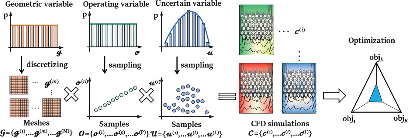
  , Figure 6.1) until one that is best-performing is found by evaluating the outputs of all objectives {obj1,…Objk…,ObjK}. For each solution, to accurately capture the multi-phase fluid flow and interfacial heat and mass transfer, it is often required to build a high-fidelity numerical model by solving the first-principle governing equations via mesh-based methods [7–9] (e.g. finite volume method and finite element method) with the aid of computational fluid dynamics (CFDs) tools. In practice, however, it is well known that numerical modeling is time-consuming, especially for varying geometry design problems that require tedious preprocessing and calibration procedures such as mesh regeneration or calibration of initial and boundary conditions [10]. Hence, the resulting computational burden becomes a major bottleneck that slows down the research and development of cutting-edge heat exchange designs.
6.2 PINN-Based Inverse Design Method
6.2.1 Overview of Inverse Design


 i and
i and  j denote the general form of the PDE operator and boundary condition operator, respectively; N
 and N
and N are the numbers of corresponding equations involved in the PDEs and boundary conditions. ∂Ω denotes the boundary of domain Ω that is required for defining the constraints. Generally,
  j may consist of differential, nonlinear, and identity terms, which could be subject to the following Dirichlet and Neumann boundary conditions [44], as given by


6.2.1.1 Standard Physics-Informed Neural Networks

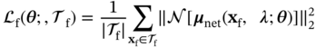
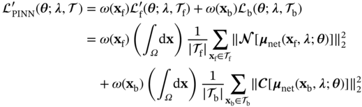
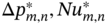
![A structure illustrates a Physics-Informed Neural Network P I N N framework for the design of heat exchangers. It represents the neural network with inputs x and lambda and theta as the network parameters. The neural network outputs variables u, rho, and T. P D Es governing the physical system, with lambda as a parameter. The equations are N [f(x); lambda]=0 and C[f(x subscript b); lambda]=0. Here, N and C are operators.](/wp-content/uploads/2025/05/c06f002-1.png)
 = [x1,…,x∣
  ∣] to satisfy the physics imposed by the PDEs and boundary conditions. For this purpose, a composite loss function that penalizes the divergence of the neural network from the PDEs and boundary conditions is considered.

 f and
f and  b, are the sampled points in the domain and on the boundary, respectively,
  f ⊂ Ω,
  b ⊂ ∂Ω,
  = [
= [ b,
b,  f]. Since the loss function is often highly nonlinear and non-convex, the network parameters θ of PINN are iteratively optimized by gradient-based optimizers, such as gradient descent, Adam, and L-BFGS [45].
6.2.1.2 Design Optimization and Decision-making Methods
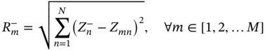
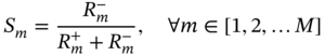
 denotes the mth alternative solution in terms of the nth objective, and
  denotes the maximum value of all the alternative solutions in terms of the nth objective. Ymn denotes the element of the positive matrix Y.
6.3 Example 1: Finned Heat Sink Model
6.3.1 System Description and Objectives
Property
ρ (kg m−3)
κ (W (m K)−1)
Cp (J (kg K)−1)
μ (kg (m s)−1)
Fluid
1.0
1.0
50
0.02
Solid
1.0
5.0
80
—

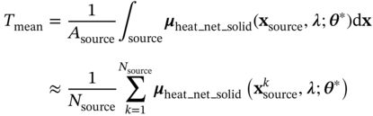
 ,
,  , and
, and  are the coordinates of samples collected on the heat source surface, channel inlet, and outlet sections, respectively; Nsource, Nin, and Nout are the corresponding numbers of these samples.
Variable/constraint
Unit
Lower bound
Upper bound
Operating variable, λ(2)
Inlet air velocity
Uinlet
m s−1
0
3.0
Design variable, λ(1)
Fin height
H
m
0
0.6
Fin thickness
D
m
0.05
0.15
Central fin length
Lctrl
m
0.50
1.0
Side fin length
Lsd
m
0.50
1.0
Process constraint
Inlet air temperature
Tinlet
°C
20
Heat flux
qs
W m−2
1800
Max allowable junction temperature
Tmax
°C
90
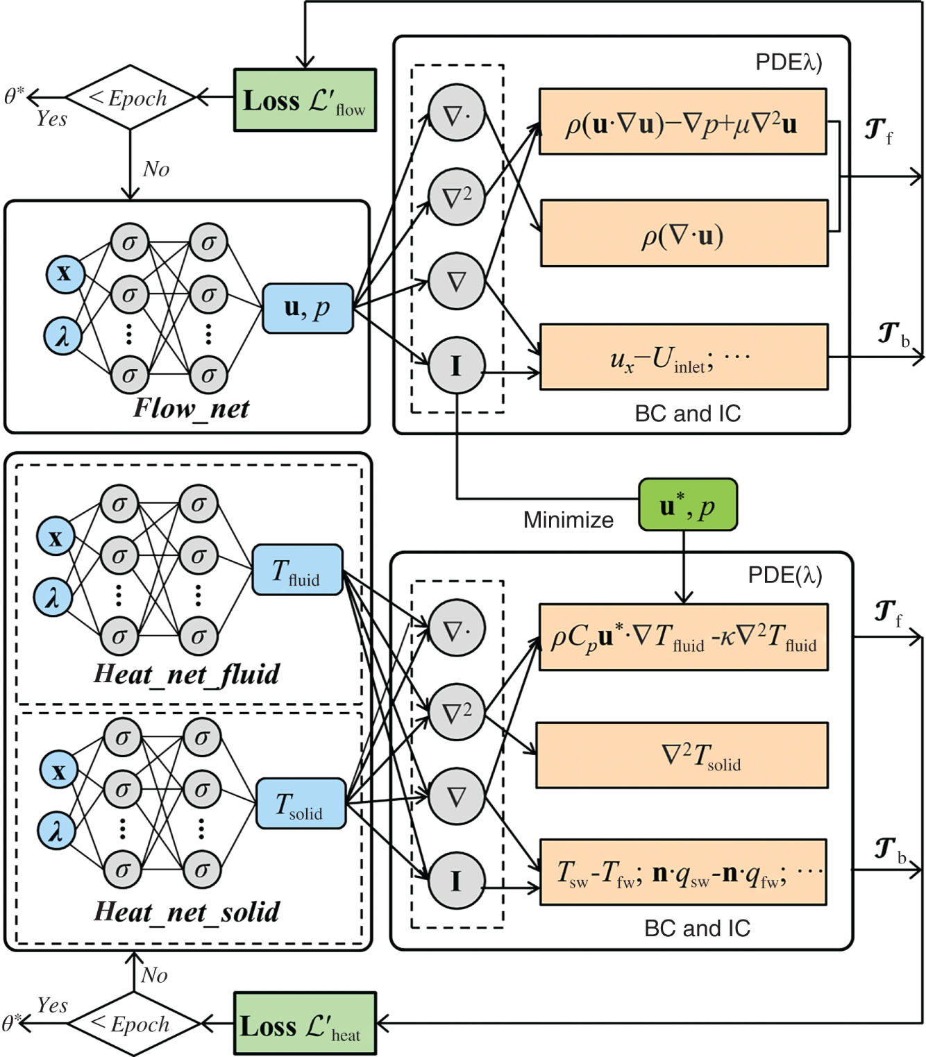
6.3.2 Improved PINN Structure
6.3.3 Results
NMAPE
ux (m s−1)
uy (m s−1)
uz (m s−1)
0.88%
1.14%
0.40%
p (Pa)
Tfluid (°C)
Tsolid (°C)
1.53%
4.17%
0.38%
Δp (Pa)
Tmean (°C)
Tpeak (°C)
CFD
9.137
68.51
78.10
PINN
9.178
70.34
79.38
Relative error
0.45%
2.66%
1.64% 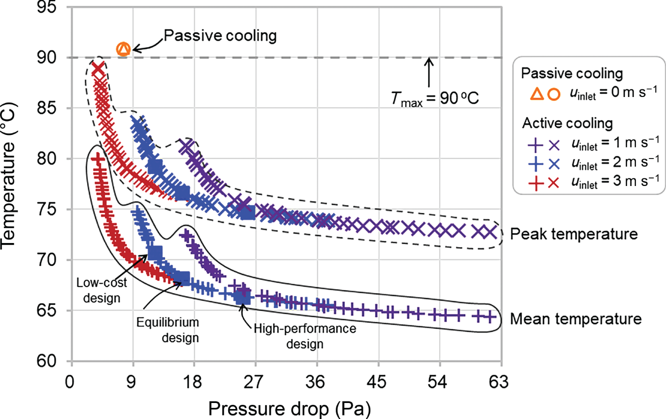
6.4 Illustrative Example 2: Tubular Air Cooler Model
6.4.1 System Description and Objectives
 ,
,  , and
, and  are listed in Table 6.4.
Input variables
Symbol
Unit
Lower bound
Upper bound
Geometric variables

Transverse tube pitch
ST
m
2D
4D
Longitudinal tube pitch
SL
m
3D
5D
Cross tube pitch
SC
m
−5D
5D
Tube diameter
D
m
0.01
Operating variables

Velocity of inlet air
Uin
m s−1
1
2
Uncertain variables

Dry-bulb temperature of inlet air
Tin
K
259.15
306.15
 . That is, the entire design space is represented using M discrete geometric designs, and each design
  represents a combined set of geometric variables. Meanwhile, the uncertainty of weather conditions is realized by extracting N uncertain samples that can represent the actual environment, and these samples are fed into each optimization model. We employ a non-intrusive sampling approach called the stochastic reduced-order model (SROM, see details in Chapter 8) to generate a finite set of stochastic samples with varying probabilities,
  (n)∈
(n)∈ ,
,  (n) = {ℴ(n),
  (n)}.
(n)}.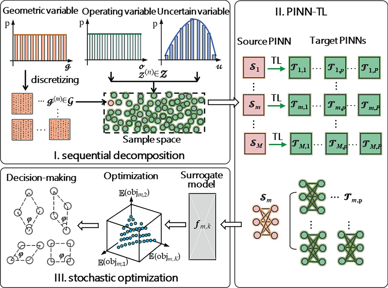

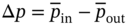 is the pressure drop between the inlet and outlet of airflow in the computational domain, and ha is the air-side convection heat transfer coefficient that can be calculated from:
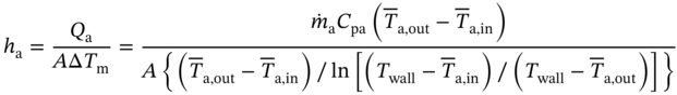
 and
and  are the mean temperatures of air at inlet and outlet, Twall is the temperature of the tube wall.
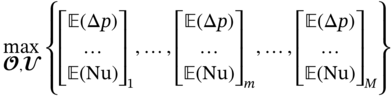
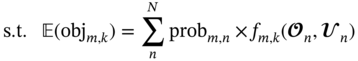

 n and
n and  n are the realizations of operating and uncertain variables in a specific sample n; lb and ub are the corresponding lower and upper bounds for these variables; probn is the probability related to the occurrence of a specific sample n; 𝚿 is the design constraint that defines the outlet temperature of the hot fluid to meet the cooling requirement. fm,k (·) is the surrogate model corresponding to the kth objective under mth geometric design, which is used as the objective function depending on the operating and uncertain variables.
 } are generated by repeatedly solving this optimization model for M × N times according to the numbers of uncertain samples and geometric designs. Similar to example 1, the NSGA-II [54] is also adopted to handle each optimization problem since it can efficiently search for the Pareto solutions. After that, the TOPSIS method is applied to identify the optimal operating conditions for each uncertain sample and determine the expected value of the optimal objective function
  for each geometric design. Finally, the most preferred solutions regarding the best-performing geometric design {
 } are obtained by re-applying with the TOPSIS method.
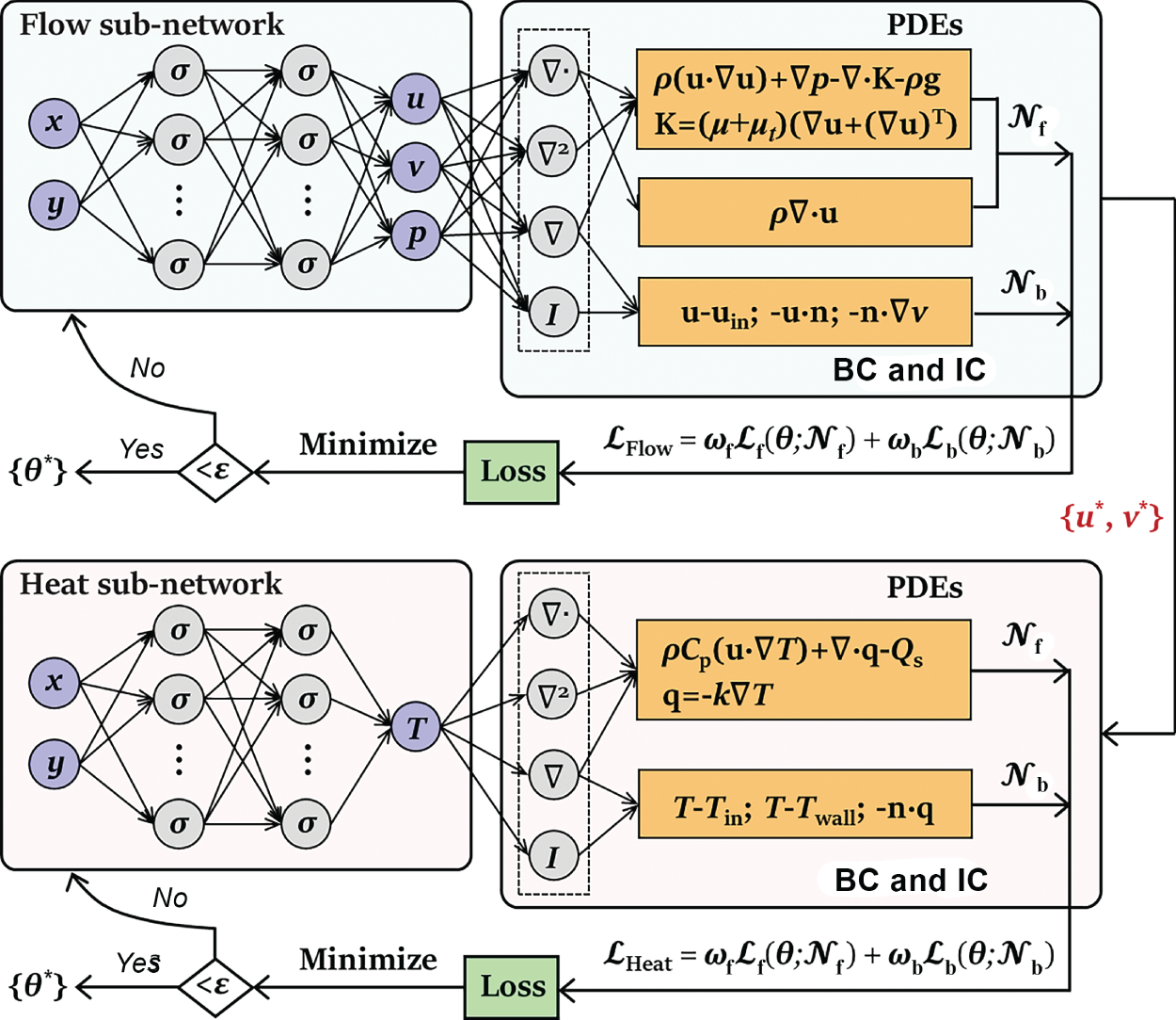
6.4.2 Improved PINN Structure
6.4.3 Transfer Learning
 S = {
S = { S, P(XS)} and learning task
  S = {
S = { S, fS (·)}, a target domain
  T = {
T = { T, P(XT)} and learning task
  T = {
T = { T, fT (·)}, it aims to improve the learning of the target predictive function fT(·) using the knowledge in
  S and
S and  S, where
  S ≠
S ≠  T or
T or  S ≠
S ≠  T;
T;  and
and  are the feature and label spaces; P(X) is a marginal probability distribution, where X ∈
  . In this study, we perform design space exploration and operating parameter optimization tasks, which are based on constructing a surrogate model using the solutions obtained from a batch of PINN models. In theory, neural network solvers can transfer knowledge across these PINN models via transfer learning since both source PINN and target PINN originate from the decomposition of the same design space of the heat exchanger system. Here, a parameter-transfer learning approach that assumes
  S and
S and  T share partial parameters or prior distributions of the hyper-parameter of the source model is employed, where the transferred knowledge acquired by a source PINN for a specific geometry is encoded into the shared parameters or priors. By discovering the shared parameters or priors, the acquired knowledge can be applied to the construction of target PINN models that have similar geometry and slightly different operating and uncertain conditions.
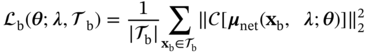
 . The parameters of these two sub-networks are tuned by minimizing the following combined losses
  and
and  . The trained optimal network parameter set
  is further used for the initialization of network parameters for each target PINN model. Based on the sample set
  , the initialized target PINN model is then re-trained to cope with the changes in operating and uncertain conditions without having the NN model trained from scratch. In this stage, the parameters of two similar sub-networks in the target PINN models are fine-tuned by minimizing the combined losses,
 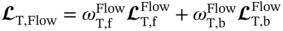 and
and  , with a limited number of iterations, smaller learning rate, and a faster learning rate decay, as listed in Table 6.5. Iteratively,
  is updated and
 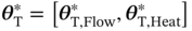 is obtained at the end of this stage.
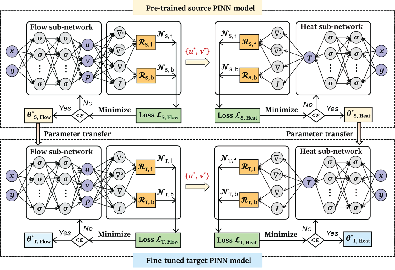
Source PINN
Parameters
Flow
Heat
Target PINN
No. neurons
256
256
256
No. layers
6
6
6
Learn rate schedule
Exponential decay
Exponential decay
Exponential decay
Learning rate
5 × 10⁻⁴
5 × 10⁻⁴
1 × 10⁻⁴
Decay step
15 000
8000
3000
No. iterations
1.5 × 10⁶
0.8 × 10⁶
0.3 × 10⁶
Activation function
Swish
Swish
Swish
Optimizer
Adam
Adam
Adam
 T| for training the target PINN models. Herein, we propose a point density adjustment (PDA) strategy that can quickly identify an optimal ratio of sample size in the domain to that on the boundary by comparing different sampling schemes. For example, the size of residual points on the boundary remains constant (|
 T,b| = |
 S,b|), while the proportion of interior residual points drops gradually.
6.4.4 Results
Outputs
FCN
FN
MFN
u (m s−1)
6.67%
2.57%
1.54%
v (m s−1)
32.99%
9.47%
4.60%
p (Pa)
16.95%
10.60%
6.80%
T (K)
64.14%
6.22%
3.15% 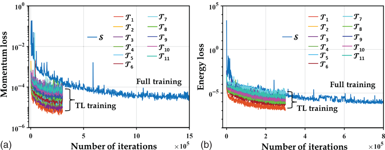
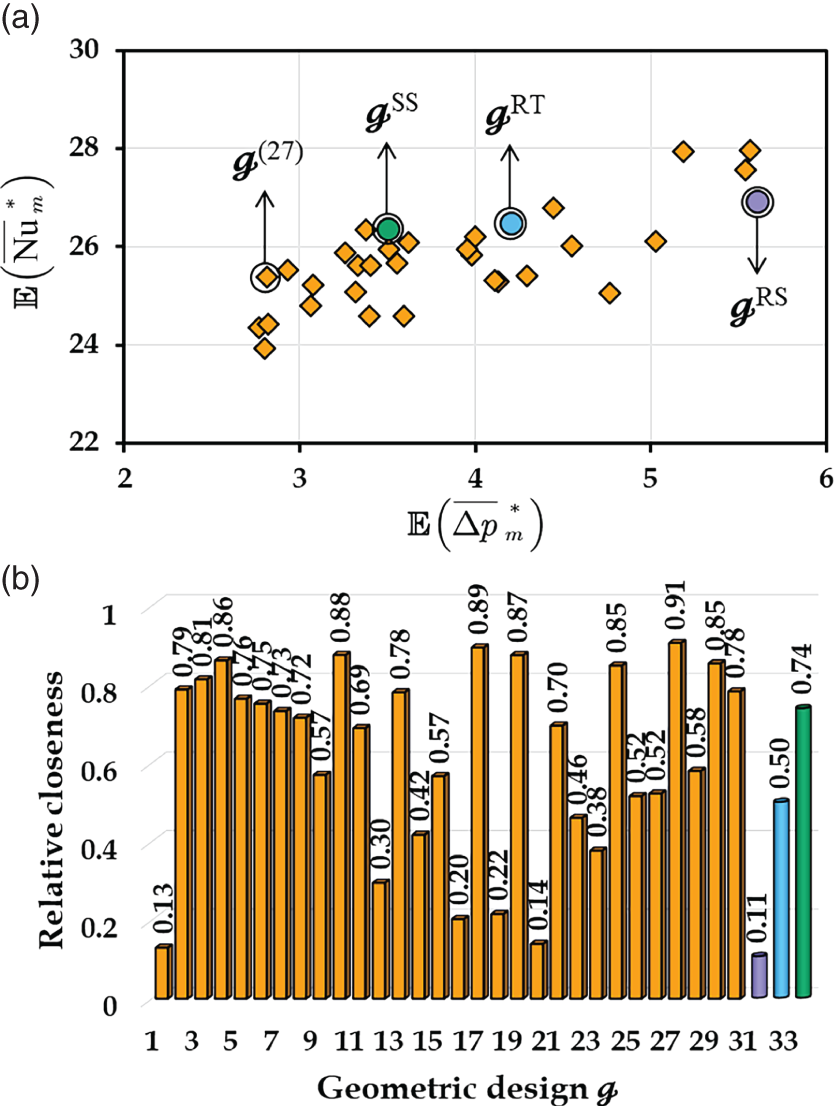
 (27), where
  = 25.38 and
  = 2.81 Pa. For a better comparison, three representative topology designs (see Figure 6.9d) often used in actual engineering design and manufacturing are also evaluated, namely rotated square (
 RS, ST = 0.5SL, SC = 0.5SL, ϕ = 45°), regular triangle (
 RT, ST = √3/2SL, SC = 0.5SL, ϕ = 60°), and standard square (
 SS, ST = SL, SC = 0, ϕ = 90°). The expected Nusselt numbers for
  RS,
RS,  RT, and
  SS are 26.92, 26.47, and 26.37, which is 6.07%, 4.29%, and 3.90% higher than that for (27), respectively. Meanwhile, the expected pressure drop for (27) has a dramatic rise from 2.81 to 5.61 Pa for
  RS, 4.20 Pa for
  RT, and 3.51 Pa for
  SS. Figure 6.13b shows the relative closeness of each design point with their corresponding values. Herein, a larger value of relative closeness means a closer distance to the ideal solution and a further distance away from the nadir solution. The relative closeness of the (27) has the largest relative closeness (0.91) as compared to the other geometric designs; therefore it is recommended as the most preferred solution for the case study.
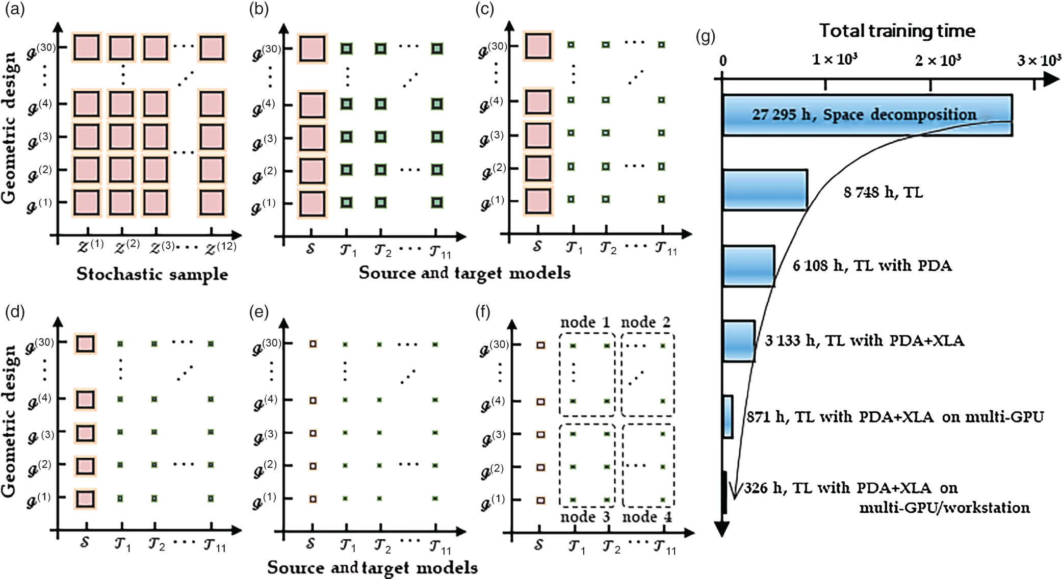
 RS,
RS,  RT, and
  SS with respect to the optimal tube arrangement. As depicted, the value of transversal tube pitch ST in (27) is ST = 0.0369 m, which is greater than that in
  RS (ST = 0.02 m),
  RT (ST = 0.026 m), and
  SS (ST = 0.03 m). Notably, the (27) has nearly the same longitudinal tube pitch SL = 0.0302 m as compared to
  RT (SL = 0.03 m) and
  SS (SL = 0.03 m). Among them, the
  RS has the longest longitudinal tube pitch SL = 0.04 m. The different included angles between tubes ϕ can be formed by changing the cross tube pitch SC. To be more specific, the value of SC is SC = −0.0056 m in (27), and an included angle of ϕ = 98.6° is formed, which is greater than that in
  RS (SC = 0.02 m, ϕ = 45°),
  RT (SC = 0.015 m, ϕ = 60°) and
  SS (SC = 0 m, ϕ = 90°).
 RS,
RS,  RT, and
  SS have nearly the same optimal solutions, and the corresponding expected values are 1.67, 1.64, 1.66, and 1.65 m s−1, respectively. It is seen from Figure 6.15c that, the optimal pressure drops for all samples in
  RS,
RS,  RT, and
  SS increase from 3.43 to 7.30, 2.49 to 5.34, and 2.07 to 4.49 Pa, respectively, which are higher than the case of
  (27) that grows from 1.79 to 3.52 Pa. This is mainly attributed to the fact that (27) has a wider flow channel, leading to a smaller pressure drop. In Figure 6.15d, the optimal Nusselt numbers for all samples in the (27) increase from 20.01 to 30.03, which are slightly lower than that in the
  RS (21.55–30.05),
  RT (20.82–30.58), and
  SS (20.61–30.44). This is because a larger ST leads to larger fully developed regions with a smaller Nusselt number. It should be noted that the effect of ST on the Nusselt number is less than that on pressure drop.
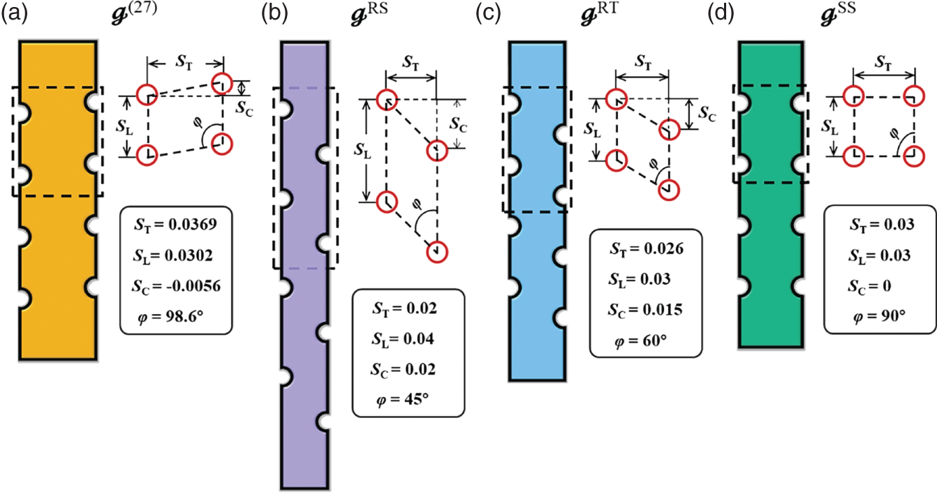
 RS), (c) regular triangle (
 RT), and (d) standard square (
 SS).
SS).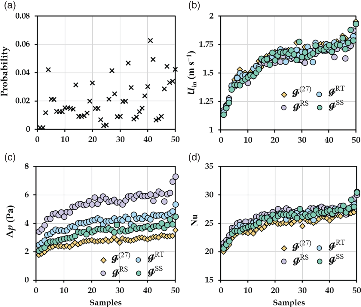
 RS,
RS,  RT, and
  SS. (a) The probability of occurrence, (b) pressure drop, (c) Nusselt number, and (d) inlet air velocity. All samples are rearranged in ascending order of the dry-bulb temperature of inlet air.
6.5 Conclusion
References
Reverse Design of Heat Exchange Systems Using Physics-Informed Machine Learning
(6.1)
(6.2)
(6.3)
(6.4)
(6.5)
(6.6)
(6.7)
(6.8)
(6.9)
(6.10)
(6.11)
(6.12)
(6.13)

(6.17)
(6.18)
(6.19)
(6.20)
(6.21)
(6.22)
(6.23)
(6.24)
(6.25)
(6.26)
(6.27)
(6.28)

(6.30)
(6.32)
(6.33)
(6.34)
(6.35)
(6.36)
(6.37)
(6.38)