Lynne C. Kaley Pinnacle, Houston, TX, USA The use of risk-based inspection (RBI) for pipelines is increasing in demand as government regulators worldwide are requiring operators to use risk assessment in high-consequence areas. Historical statistics attribute piping failure as the leading cause of large property losses globally [1]. Data from numerous corporations indicate that the most frequent failures (approximately 35–40%) are from piping systems. There are a number of international design codes and standards covering pressurized equipment that should be referenced when considering a piping program. The Norsk Sokkels Konkuranseposisjon (NORSOK) standards, developed by the Norwegian petroleum industry, were intended to supersede individual company specifications as a reference for government regulators. ISO 31000, Risk Management—Principles and Guidelines, is a family of international risk management standards that provide generic guidance for any risk management implementation. Other ISO and OGP standards focus more specifically on risk and integrity management specifications and techniques. This chapter focuses on in-service American Petroleum Institute (API) codes and standards that were developed by representatives from multinational oil and gas companies through an ANSI-accredited balloting process. API 510, 570, and 653 and associated documents define inspection requirements for pressurized equipment, while recommended practices API 580 and 581 provide the necessary guidance on RBI programs and methodology. RBI methods and applications for inspection planning, execution standards, and recommended practices are also described by American Society of Mechanical Engineers (ASME). Finally, the assessment of fitness-for-service and remaining life (RL) using API 579-1/ASME FFS-1 can be used to justify continued service when damage is found during inspection. Risk-based principles allow low-risk and low-consequence systems to run to failure. This risk concept implies that other systems are high in risk and that the consequence of failure (COF) is unacceptable; as such, these systems should receive attention even when the probabilities of failure are not significantly high. Risk-based principles challenge accepted design codes that are based on deterministic design and fitness-for-service codes, particularly where worst-case scenarios are used without consideration for COF. Differences in inspection requirements and remedial action will occur when deterministic methods are compared with recommendations from risk-based methodologies. The purpose of a RBI program is to develop risk assessment in order to implement an integrity inspection program over a defined period with the available data and detailed technical data. With inspection planning focused on high-risk items, inspection generates the necessary technical data required for risk assessment updating and fine-tuning future priorities. RBI methodologies can be used on older facilities that have little or poor data available; on newer assets where technical data are available, but little inspection history exists; and on facilities with good quality data and inspection history. A RBI program should be considered for the following pipeline assets: Since facilities range widely in age, there is often limited construction, process, and inspection history available. Inspection and maintenance programs are sometimes reactionary, lacking a cohesive strategy or long-term plan based on expected in-service damage to equipment. Construction and process data and inspection histories are marginal or missing completely. The quality of available information on the assets determines whether a qualitative or quantitative RBI approach should be used. Less data generally require a more qualitative approach, at least initially. The approach adopted will depend on the following: Regardless of the approach used, a continuous improvement process similar to one of the following should be implemented: As the program develops and matures, a more quantitative analysis can be incorporated, as desired. This chapter is primarily intended to be used for the planning of in-service inspection for pipeline static mechanical pressure systems when considering failures by loss of containment of the pressure envelope. Failure modes, such as failure to operate on demand, leakage through gaskets, flanged connections, valve stem packing along with valve passing, and tube clogging, are not addressed. The focus is on pipeline pressure systems involving the following types of components: Excluded from the scope are In this chapter, “equipment” is defined as any of the aforementioned, while a “system” refers to a combination or group in the aforementioned list. Traditional risk analysis and risk management is based on applying a systematic approach to use available knowledge to assess, mitigate (to an acceptable level), and monitor risk. The goal is to identify all reasonably foreseeable detrimental impacts on asset integrity and reliability. Risk is assessed by identifying possible failures, estimating the probability of failures (POFs), and assessing the COFs. The results of the risk assessment are then used to reduce the impact of failure to as low as reasonably practicable (ALARP). The risk management process is a continuous activity that reflects changes in the operating environment and the need to monitor and maintain the performance of the resources. The major concepts of a traditional risk analysis process comprise five tasks: A typical risk analysis scenario includes the following set of events: loss of containment; detection, isolation, and mitigation. Depending on the nature of the process and the detail of the study, a risk analysis can include thousands of different scenarios with evaluation of both the probability and the consequence of the set of events in each scenario. In the system definition phase of a risk analysis, the ground rules are established and all pertinent information is collected. The ground rules of the analysis typically include the following: A critical step is to identify hazards that can cause injury to humans, damage to the environment, damage to property, or loss in production. The hazards are identified along with how the hazard can develop into an accident, the consequences of a potential accident, and the safeguards in place to prevent an accident. The major focus is to evaluate various scenarios that may lead to undesirable outcomes. Both the probability and the magnitude of these outcomes are estimated and displayed as results. A hazard and operability study (HAZOP) is a structured brainstorming exercise that uses a list of guide words to stimulate team discussion. The guide words initially focus on process parameters (such as flow, level, temperature, and pressure) and then branch out to include other concerns such as human factors and operating outside normal parameters. The majority of identified potential deviations are typically operability issues, but potential safety concerns and environmental considerations are also identified. For maximum effectiveness, the HAZOP is typically performed by a team familiar with the process rather than an individual. This team normally needs participation from various disciplines, including mechanical design, instrumentation, machinery, and metallurgy. The task of hazard identification has received much public attention and, as a result, is one of the most mature of the various disciplines that comprise a risk analysis. A probability assessment is conducted to estimate the probability of occurrence for the scenarios identified in the previous phase of the risk analysis. If a scenario occurs fairly frequently, it is best to use historical data to estimate the event’s probability. However, if the events are rare and sufficient data do not exist to estimate their probability based on the historical data alone, a building-block approach is used. Probability estimates for all elements of the scenario are obtained and combined to predict the overall scenario probability. The most common measure of probability for a scenario is frequency. A single fixed value is assigned for the frequency/probability term and is considered constant over time. Frequency can be used for a single event or a series of events. A year is most often used as the standard time interval for a frequency analysis. Frequencies may be very small numbers, such as one in a million years for infrequent events, or they may be relatively high values, such as once a month or four times a day. If, for example, a pipe is known to leak about every 5 years, it would have a leak frequency of one in 5 years or 0.2 per year. The term “recurrence period” is sometimes used to refer to the reciprocal of the frequency. In our example, the recurrence period for the leak would be 5 years. To obtain the frequency of the scenario, multiply the frequency of the leak by the probability of all events that follow. The resulting likelihood is the scenario’ s frequency. The mathematical representation of the likelihood of the sequence, in terms of frequency, is as follows: For example, consider a leak that does not ignite. If the estimated leak frequency is 10−5 and the probability of that leak not igniting was 0.5, the overall frequency for the no ignition scenario is 10−5 × 0.5 = 5 × 10⁻⁶. The consequence of a release from equipment varies depending on factors such as the physical properties of the material being handled, toxicity or flammability characteristics, weather conditions, release duration, and mitigation actions. The effects may impact plant personnel or equipment, nearby population, and the environment. Hazardous consequences are estimated in five phases: Depending on the material released, only one of the flammable, toxic or, environmental effects is calculated, although all of them may be possible with the release of certain mixtures. Historically, a number of measures have been used to express risk in the context of a risk analysis. There is no single way to measure or present an estimate of the risk of an operating process. Risks to people are normally presented in one of the three ways: risk indices, individual risk measures, and societal risks. Risk indices are a single number measure of risk. Some of the more common risk indices are as follows: Individual risk measures consider the risk to an individual who might be located at any point in the effect zones of incident. Following are some of the more common individual risk measures: Societal risk is a measure of risk to a group of people in the effect zones of incidents. It is most often expressed in terms of the frequency distribution of multiple fatality events. RBI is a methodology that uses risk as a basis for prioritizing and managing the efforts of an inspection program, including recommendations for monitoring and testing inspection plans. It provides focus for inspection activity to specifically address threats to the integrity of the asset and the equipment’s capacity to operate as intended. The POF and COF are assessed separately and then combined to calculate risk of failure. Risk is compared and equipment risk prioritized for inspection planning and risk mitigation. A RBI program includes the following: A RBI program is not a fully quantitative risk analysis, but a technique that combines the disciplines of risk analysis and mechanical integrity. However, the techniques used in RBI are similar to those seen in traditional risk analysis. RBI methodology follows the five tasks of a traditional risk analysis described in the previous section, but it uses a modified and in some cases simplified approach: RBI focuses on the development of inspection programs to address damage types that inspection should detect; the appropriate inspection technique to detect the damage; and the application of RBI tools to reduce risk and optimize the inspection program. Figure 67.1 Risk matrix example. Figure 67.2 Iso-risk example. Inspection influences risk primarily by reducing the POF. Many conditions (design errors, fabrication flaws, and malfunction of control devices) can lead to equipment failure, but in-service inspection is primarily concerned with the detection of progressive damage. RBI considers that the POF is due to damage as a function of four factors: RBI differs from conventional inspection management because it provides the concepts and methods to support decision making even when data are missing or uncertain. Rational decisions can be made using both quantitative and qualitative RBI methods. The benefits of using RBI for inspection planning are as follows: The inspection planning process directs resources to accurately determine the condition of the equipment through the most effective and efficient inspection methods, balancing the necessary down time and cost of inspection against the effectiveness and benefits of inspection. Operators considering a piping inspection program should be aware of several important industry design codes and standards that cover pressurized equipment. The API in-service codes and standards, including API 510, API 570, and API 653, and their associated documents should be used to define inspection requirements for pressurized equipment and tanks. Recommended practices API 580 and API 581 provide the necessary guidance on RBI programs and methodologies. RBI methods and applications for inspection planning, execution standards, and recommended practices are also described by ASME PCC-3-2007 Inspection Planning Using Risk-Based Methods. Finally, assessment of fitness-for-service and RL using API 579-1/ASME FFS-1 can be used to justify continued service when damage is found during inspection. ASME PCC-3-2007 provides guidance on the preparation and implementation of a RBI plan based on API RP 580 RBI, the earliest industry standard on the practice. ASME PCC-3 and API RP 580 are closely aligned as changes, additions, and improvements are made to each document to enhance applicability for a broader spectrum of industries. ASME-PCC-3-2007 provides recognized and generally accepted good practices that may be used in conjunction with postconstruction codes, such as API 510 and API 570. The purpose of API RP 580 is to provide users with the basic elements required for developing, implementing, and maintaining an RBI program. The risk analysis principles, guidance, and implementation strategies presented in this document are broadly applicable but were specifically developed for applications involving fixed pressure-containing equipment and components. API RP 580 provides guidance to owners, operators, and designers of pressure-containing equipment for developing, implementing, and assessing inspection programs. API RP 580 emphasizes safe and reliable operation through cost-effective inspection using a spectrum of complimentary risk analysis approaches (qualitative through fully quantitative) as part of the inspection planning process. API RP 580 includes an introduction to the concepts and principles of RBI for risk management as well as the steps that should be followed in applying risk management principles within the framework of the RBI process. These steps include the following: The expected outcome from an RBI process should be the association of risks with appropriate inspection, process control, or other risk mitigation activities to manage the risks. The RBI process is capable of generating API RP 581 [2] was developed to provide users with a specific approach for developing, implementing, and maintaining a RBI program. The methodology outlined in API RP 581 [2] was developed through a joint industry project initiated in May 1993 and conducted by API to develop practical methods for RBI. The original sponsor group was organized and administered by API and included the following original members: Amoco, ARCO, Ashland, BP, Chevron, CITGO, Conoco, Dow Chemical, DNO Heather, DSM Chemicals, Exxon, Fina, Koch, Marathon, Mobil, Petro-Canada, Phillips, Saudi Aramco, Shell, Sun, Texaco, and UNOCAL. The results of this project were published in a RBI base resource document (BRD) to the sponsor group based on the development of quantitative and qualitative RBI methodologies. The methodologies developed in the project continue to be improved and maintained in API RP 581 [2]. The target audience in the proposal for the API sponsor group project stated that the methods in it were “to be aimed at an inspection and engineering function audience.” The methodology was specifically not intended to “become a comprehensive reference on the technology of quantitative risk assessment (QRA).” For failure rate estimations, the proposal promised “methodologies to modify generic equipment item failure rates” via “modification factors.” For consequence calculations, safety, monetary loss, and environmental impact were to be included. Existing algorithms in AIChE chemical process quantitative risk analysis (CPQRA) guidelines are “complex and are best suited for use in a computerized form” for safety evaluations. It was proposed that “for ease of use, that safety consequences be limited to the evaluation of burning pools of liquids, ignited high-velocity gas and liquid releases, explosions of vapor clouds, and toxic impacts.” The result of the sponsor group project and subsequent activities has been the development of simplified methods for estimating failure rates and consequences of pressure boundary failures. The methods are aimed at persons who are not expert in QRA. Subsequent computer programs were developed to further ease the application of the BRD and now API RP 581 [2] methodologies. The approach outlined in API RP 581 [2] has been successfully implemented in major refineries, petrochemical/chemical plants, and upstream gas plants. In recent years, an increasing emphasis on pipeline process safety management and mechanical integrity using RBI has been considered for all upstream and pipeline applications following established and emerging OSHA, DOT, and API regulations and recommended practices. Equipment or system failure and the subsequent release of hazardous materials can lead to many undesirable effects, including the unavailability of equipment. A RBI program considers these effects based on four basic risk categories: The risk calculation is performed for each scenario, for all four risk categories, if desired. The risk for each equipment item is then found by summing the individual risk components from each scenario (hole size) calculation. RBI begins with the identification of high-risk assets followed by the assessment of equipment condition, evaluation of maintenance and inspection programs, study of operating protocols, and estimation of life consumption of these priority assets. This process takes into account the probability and consequences of mechanical failure. The information is used to modify and optimize inspection and maintenance programs, audit procedures, operating limits, and safety information. The POF due to loss of containment should consider each of potential degradation mechanism that could lead to loss of containment. POF (loss of containment) can be estimated quantitatively, if any degradation model exists, or qualitatively by means of engineering judgment. Given that loss of containment has occurred, the potential consequences depend on the size of the hole, which can vary from a pinhole to a full-bore rupture. The methodology’s handling of hole size probability distribution by degradation mechanism should be understood when considering the potential consequences of any loss of containment, since the approach used can significantly affect the outcome. Finally, the probability that loss of containment can lead to ignition or pollution is an important issue. RBI can be carried out using methods that are qualitative or more quantitative. In practice, most RBI efforts are carried out using a blend of both the methods, referred to as semiquantitative, and is often represented as a continuum as shown in Figure 67.3. The qualitative assessments can be conducted at a system or equipment level, while quantitative assessments are conducted on the equipment level, as follows: Figure 67.3 Range of RBI analysis details. Regardless of the level of assessment conducted, the team should be comprising specialists with considerable experience with the specific installation(s) being assessed and include relevant expertise in the RBI methodology being used. Since qualitative assessments are based on rankings and numerical assignment during experienced-based team sessions, a higher level of experience and specialist involvement is required for a credible assessment. In addition, the documentation of data and any assumptions that were the basis for the assessment should be documented sufficiently for the study to be reproduced at a later date, even if the original team members are not available to participate. Conversely, RBI assessments based on actual design, operating, and inspection data require less documentation and assumptions, making future reassessments more reproducible. Qualitative approaches are similar to quantitative analysis but require less equipment-specific data and can take less time to complete. While the results yielded are not as precise as those of the quantitative analysis, this approach provides a basis for prioritizing a RBI inspection program. However, as previously mentioned, a higher level of experience and specialist involvement is required for a credible qualitative assessment. The basis for all numerical assignments or rankings should be thoroughly documented as well as any assumptions that were the basis for the assessment in the event that the original team members are not available to participate. Qualitative models can be interpreted as an expert judgment-based approach in which a numerical value is not calculated or assigned. A descriptive ranking is given, such as low, medium, or high, or a numerical ranking such as 1, 2, or 3. Qualitative RBI approaches cover a wide spectrum of methodologies. The simplest approach would be to compile the data/information required to do a quality damage review for the POF and categorize the hazards for COF to generate a risk matrix location to recommend a relevant inspection frequency. The advantage of using a qualitative approach is that the assessment can be completed quickly and at a lower initial cost; there is little need for detailed information and the results are easily presented and understood. A disadvantage is that the results are more subjective than quantitative analysis because they are based on the opinions and experience of the RBI team and are thus harder to update the following inspection. Qualitative models provide a risk ranking of items since there is no change in risk over time and setting an acceptable risk target is not possible. As a result, an inspection interval is assigned based on position in a risk matrix that only changes if an input value, and therefore, matrix location changes. Methodologies that would be considered qualitative generally have the following characteristics: A qualitative analysis of a system can be conducted to quickly prioritize groups of equipment for more detailed risk analysis. The result of any qualitative analysis positions equipment within a risk matrix and provides a method for risk rank prioritization. This level of qualitative analysis is performed at any of the following levels: Note that the aforementioned four levels are most representative of an oil/gas separation plant. Pipeline applications would generally only apply to the system and equipment levels. Qualitative approaches conducted at the system level are generally influenced by the number of equipment items in the system or equipment being studied because the quantity and type of inventory is considered to assign COF. As a result, assessments conducted at the system level should be based on similar equipment counts when used to compare systems for prioritization purposes. Equipment level qualitative assessments do not require any special considerations for risk prioritization purposes. Qualitative RBI procedures have the following three functions: The qualitative analysis determines a risk ranking for systems or equipment by categorizing the two elements of risk: POF and COF. The process involved and the physical boundaries of the study area must be defined before the qualitative analysis is conducted. The following sections provide an overview of the factors that should be considered in any qualitative analysis. POF category is determined by estimating the susceptibility of the system/equipment to one or more degradation mechanisms that affect the probability of a leak. An adjustment is made to the POF category based on the known condition of the system/equipment, inspection program history, and process stability and design considerations. Key factors that may be considered to determine the POF based on equipment type are as follows: These components are combined to determine the final POF and POF category. POF is plotted on the vertical axis of the risk matrix (see Figure 67.1). The DF is a measure of the risk associated with known or potential degradation mechanisms. The potential degradation mechanisms include levels of internal (corrosion or cracking), external (corrosion or cracking), and mechanical damage (fatigue and brittle fracture). The inspection factor provides a measure of the effectiveness of the current inspection program and the ability of the program to detect and quantify active or anticipated degradation. It is based on inspection methods, coverage, and inspection program management. The inspection factor is weighted with negative numbers because the quality of the inspection program will partially offset the POF inherent in the degradation mechanisms from the DF. The current equipment condition factor is a measure of the physical condition of the equipment from a maintenance and housekeeping perspective. Simple evaluations are performed on the condition and upkeep of the equipment from a visual examination. The process factor is a measure of the process stability and potential for abnormal operations or upset conditions that may initiate a sequence of events leading to a loss of containment. It is a function of the process interruptions, stability of the process, and potential for failure of protective devices because of plugging or other causes. The equipment design factor evaluates the factor of safety equipment design, whether it is designed to current standards and the complexity of design. There are two major potential hazards associated with pipeline operations: (a) fire and explosion risks, flammability and (b) toxic risk. In determining the toxic consequence category, RBI considers acute and does not consider chronic effects. The key variables that affect flammable consequences are process composition, available inventory, and state in the process (liquid, gas, or mixed phase). These three variables can be combined to determine flammability COF. Operating temperature and pressure can be used to further refine the COF. The COF analysis determines a damage consequence factor and is usually determined for each process. Many processes, however, exhibit a predominate risk (either fire/explosion or toxicity); thus if the predominant risk for a given process is known, the factor for risk should be based on the known predominant risk. If there are several processes present in relatively large percentages in the area, the risk factor for each of the processes present should be considered. In general, a good practice is to determine risk for any processes with high health consequence in addition to any that comprise at least 90–95% of the total mass of process in the area. The COF category is derived from a combination of seven elements that determine the magnitude of a fire and/or explosion hazard: The process factor, a process stream’s inherent tendency to ignite, is derived as a combination of the material’s flash factor and its reactivity factor. Flash factors correspond to the material’s NFPA 1 Class rating, while the reactivity factor is a function of how readily the material can explode when exposed to an ignition source. The inventory factor represents the largest amount of material that could reasonably be expected to be released from a unit in a single event. This factor is based on the largest mass of flammable inventory in the unit. The state factor is a measure of how readily a material will flash to a vapor when it is released to the atmosphere. It is determined from a ratio of the average process temperature to the boiling temperature at atmospheric pressure (using absolute temperatures in the ratio). The autoignition factor accounts for the increased probability of ignition for a fluid released at a temperature above its autoignition temperature. The pressure factor is a measure of how quickly the fluid can escape. In general, liquids or gases processed at high pressure (>150 psig) are more likely to be released quickly and result in an instantaneous-type release, with more severe consequences than a continuous-type release. The safety factor is determined to account for the safety features engineered into the unit. These safety features can play a significant role in reducing the consequences of a potentially catastrophic release. Several aspects of unit design and operation are included in this factor: The damage potential factor determines the potential for a fire or explosion to cause adjacent equipment damage. This is accomplished by a rough estimate of the value of equipment near large inventories of flammable or explosive materials. The flammable COF category is determined by combining the aforementioned consequence factors and selecting the category based on ranges of these combined factors. The health consequence category is derived from the following elements that are combined to express the degree of a potential toxic hazard in a unit: Toxic consequences depend heavily upon the percentage of the process fluid that is toxic. Highly toxic process streams containing a portion of highly toxic components use the same key variables as for flammable COF in addition to an estimate of toxic material based on the percentage of the toxic component in the process stream. The toxic factor is a measure of the quantity and the toxicity of a material. The quantity portion is based on mass and the toxicity of the material is found using the NFPA toxicity factor. The dispersibility factor is a measure of the ability of a material to disperse. It is determined directly from the normal boiling point of the material. The higher the boiling point, the less likely a material is to disperse. A mitigation factor is determined to account for the safety features engineered into the system/equipment: The population factor is a measure of the number of people that can potentially be affected by a toxic release event. The health COF category is determined by combining the COF factors and selecting the category based on ranges of these combined factors. The business COF category is assigned by a combination of production impact, the ability to make-up product from another source and the market value of the product. The COF categories (flammable, toxic, and business) are assigned letter scores. The final COF category is the highest value plotted on the horizontal axis of the risk matrix to develop a risk rating for the unit. The POF category rating and the highest rating from damage, toxic, or business consequence categories are used to place each unit within a 5 × 5 risk matrix, as shown in Figure 67.1. The populated matrix provides a graphic indication of risk for the systems/equipment evaluated. The system/equipment with the highest risk is a candidate for further evaluation and urgency of the evaluation. Risk matrix results are used to locate areas of potential concern, suggest an inspection frequency, and determine where additional inspection or other methods of risk reduction are necessary. The results are also used to decide whether a more quantitative study would be beneficial. It should be noted that using qualitative analysis to manage risk may result in higher than necessary inspection and maintenance costs, since emphasis would be placed on high-risk items only (increased inspection and maintenance activities) and may miss emphasis on lower risk equipment (reduced inspection and maintenance activities). The shadings provided in Figure 67.1 matrix example are guidelines for determining the degree of potential risk. These shadings are not symmetrical, as they are based on the assumption that the COF will be more heavily weighted than POF in determining total risk. It is recommended that companies develop and apply criteria to determine when further risk analysis, changes to their inspection practices or mitigation is required. Quantitative models are model-based approaches where numerical values are calculated. The advantage of a quantitative approach is that the results can be used to calculate with some precision when the risk acceptance limit is reached. Quantitative methods are systematic, consistent, documented, and are relatively easy to update with inspection results. A quantitative approach generally uses a program or software to calculate risk and develop inspection program recommendations. The models are initially data-intensive but use of models removes repetitive, detailed work from the traditional inspection planning process. The types of data required for quantitative RBI analyses are represented in the flow diagram shown in Figure 67.4. API RP 581 [2] outlines a thoroughly documented quantitative approach widely used and generally accepted in the oil and gas and petrochemical industries. API RP 581 [2] is equally applicable to offshore, midstream, and pipeline industries if a quantitative methodology is desired and supported by the data requirements. The following description of quantitative RBI analysis generally follows the methodology outlined in API RP 581 [2]. The POF analysis is based on using industry generic failure frequencies (Gff) by equipment type that is modified by two factors, reflecting identifiable differences from a generic value to an equipment-specific probability of the equipment/component being studied. A calculated equipment/component equipment factor (FEquip) reflects the specific operation, potential in-service damage mechanisms, and condition based on inspection. The FEquip is a combination of a DF modified by an inspection effectiveness factor (IF). The DF is a factor calculated based on the potential in-service damage mechanisms for the equipment. The inspection IF modifies the DF based on the history of inspection, the effectiveness of those inspections, and the result/findings. The management systems factor (FMS) is based on an evaluation of the facility’s management practices that affect the mechanical integrity of the equipment. The management system evaluation tool was based on API 750 guidelines and is included as a workbook of audit questions in the API RP 581 [2]. Figure 67.4 Type of data required for quantitative RBI analysis flow diagram. The adjusted failure frequency or POF is calculated by multiplying the Gff by the two modification factors, as shown in the following equation: The database of Gff was based on a compilation of available equipment failure histories from multiple industries. From these data, Gff were developed for each type of equipment and pipe diameter. The DF evaluates the specific operating environment of the equipment/component and determines a factor unique to the equipment operating history and inspection condition. DF calculation includes a series of damage modules that assess the effect of specific failure mechanisms on the POF. The DF for thinning is determined by calculating an ar/t factor, where The ar/t factor is defined as the ratio of wall loss (years in service age, a; times damage rate, r) and furnished thickness, t. The ar/t factor is used with inspection effectiveness to determine a thinning DF using the table in API RP 581 [2] Part 2, Table 5.11. A similar table is provided for cracking mechanisms that can be found in API RP 581 [2] Part 2, Table 7.4. The damage modules serve the following functions: The FMS adjusts for the influence of the facility’s process safety management system on the mechanical integrity of the plant. The outline of the Management Systems Workbook from API RP 581 [2] is given in Table 67.1. The complete audit of the workbook can be found in API RP 581 [2] Part 2, Table 4.4. The FMS adjustment is applied equally to all equipment/component items in the study. The FMS provides discrimination between risk of equipment/components under different management practices or at different locations and management systems. However, the evaluation process can be used to improve the effectiveness of any PSM program, thereby reducing overall risk. COF of releasing a hazardous material are estimated in the following steps: Table 67.1 Management Systems Workbook, FMS Source: Adapted from Ref. [2]. Flammable, toxic, environmental, and financial impacts are calculated. Environmental consequence is calculated from the release rate or mass information. Financial consequences are calculated using the results of a combination of flammable, toxic, environmental, and business interruption. RBI considers releases as instantaneous or continuous release types. Instantaneous releases result in emptying the vessel contents in a relatively short period of time, for example, in the case of brittle failure of a vessel. Continuous releases occur over a longer period of time at a relatively constant rate. Note that the approach is simplified by modeling only instantaneous or continuous releases since many releases have characteristics of both. The outcome of a release refers to the physical behavior of the hazardous material. Examples of outcomes are safe dispersion, explosion, or jet fire. Outcomes should not be confused with consequences that refer to the adverse effects on people, equipment, and the environment as a result of the outcome. The actual outcome of a release depends on the nature and properties of the material released. A brief discussion of possible outcomes for various types of events is as follows. The following possible outcomes may result from the release of a flammable fluid: Two outcomes are possible when a toxic material is released: safe dispersal or manifestation of toxic effects. In order for a toxic effect to occur, two conditions must be met: If either of the earlier conditions does not occur, the release of the toxic material results in safe dispersal. Safe dispersal is used in risk assessment to indicate that the incident falls below the pass/fail threshold. If both of the earlier conditions exist (concentration and duration) and personnel are present, toxic exposure will occur. RBI uses two distinct types of impact criteria to estimate consequences from a given outcome: the direct effect model and the probit (short for probability unit). The direct effect model uses a pass/fail approach to predict the consequence from a given outcome. It assumes that no effect is observed if the outcome is below the predefined threshold and it assumes a single effect for any outcome above the threshold. This approach is fairly coarse since, in reality, spectrums of effects are observed for a range of outcomes. The probit is a statistical method of assessing the impact of a given consequence. It reflects a generalized time-dependent relationship for a variable that has a probabilistic outcome described by the normal distribution. The initial steps in the consequence calculation predict the outcome in terms of the physical phenomena of a process release to the atmosphere. The final step converts the outcomes to consequences. Effect models, also known as impact criteria, are used to estimate consequences from an outcome. Direct effect models are used for flammable, environmental, and financial consequences, while toxic consequences are estimated using the probit. From an environmental standpoint, safe dispersal occurs if the released material is entirely contained within the physical boundaries of the facility. If the material cannot be contained, the release of a hazardous material will result in a spill. Financial effects are calculated as the sum of the following consequences: API RP 581 [2] outlines an industry-accepted quantitative methodology for prioritizing equipment risk at the equipment/component level. The result of the quantitative analysis positions equipment/components in a 5 × 5 risk matrix in addition to calculating discrete risk values for prioritization from higher to lower risk. The POF and COF are combined to produce an estimate of risk for each equipment/component item. The equipment/components are ranked based on risk with POF, COF, and risk calculated and reported separately to aid identification of major contributors to risk or risk drivers. Guidelines are provided to develop and modify an inspection program to manage the risks identified in the risk calculation and prioritization steps. Inspection program development will be presented in Section 67.3. High-risk assets have the potential to cause serious disruption in operations or cause unplanned and extended production outages. The priority treatment of high-risk assets must be balanced by providing sufficient maintenance and inspection for other lower-risk equipment to avoid the unintended increased risk over time. The objective is to optimize the use of pipeline maintenance and inspection resources for all equipment/components over time to manage risk at the desired levels. In any system or process, a relatively large percentage of risk in an operating plant is associated with a small percentage of the equipment items. RBI shifts inspection and maintenance resources to provide a higher level of coverage on the high-risk items and an appropriate effort on lower risk equipment, by systematically combining both POF and COF to establish a prioritized list of equipment/components based on total risk. From the prioritized list, an inspection program may be designed that manages (reduces or maintains) the risk of equipment failure. The potential benefit of an RBI program is to improve the operating efficiencies of systems or processes, while improving, or at least maintaining, the same level of risk. Figures 67.5–67.7 show the impact of an RBI assessment on the inspection program. Figure 67.5 presents a comparison of the risk reduction relative to increased inspection activity associated with a typical, non-RBI program, and risk using RBI. Both plans will decrease risk as the inspection activity increases to a point where the rate of risk reduction with additional activity is low. However, the RBI-based program achieves an overall lower level of risk with the same inspection as a result of optimization of resources based on risk. It should be noted that a certain level of residual risk is inherent in any process involving hazardous materials and additional inspection will not reduce the risk below that residual risk. Figure 67.5 Impact of RBI assessment on inspection program. Figure 67.6 Impact of RBI assessment on inspection program with reduced inspection activities. Figure 67.7 Impact of RBI assessment on inspection program with refocused inspection activities. Figure 67.6 shows how refocusing inspection activities on the highest risk equipment achieve a lower risk. The lower risk is achieved in this case without additional costs to reduce the risk. Figure 67.7 demonstrates how unnecessary or low-value inspection activities can be reduced while maintaining the same risk level when inspection priorities are based on risk. Risk reduction or risk optimization is achieved several ways, including the following: RBI focuses on risk reduction through inspection planning by the development of inspection programs that address the types of damage expected and the inspection methods appropriate to detect the expected damage. Inspection influences risk by reducing the POF through improved knowledge of the equipment condition. Many conditions (design errors, fabrication flaws, and malfunction of control devices) can lead to equipment failure, but in-service inspection is primarily concerned with the detection of progressive damage. The POF due to such damage is a function of the following factors: RBI differs from conventional inspection management by providing the methods to support decision-making when the data are missing or uncertain. Rational decisions can be made using RBI methodologies and the application of decision-making applies risk reduction through inspection. The purpose of an inspection program is to define and perform the activities necessary to detect in-service deterioration of equipment before failures occur. An effective inspection program is developed by systematically identifying Equipment data that must be available to properly assess the risk include equipment design and construction, the operating process conditions, and the maintenance and inspection history. The following basic data are required to identify damage mechanisms of interest: Design and construction data Operating process data Damage types are the physical characteristics of damage that can be detected by an inspection technique. Damage mechanisms are the corrosion or mechanical actions that produce the damage. Table 67.2 describes some familiar damage types and their characteristics. Tables 67.3–67.6 illustrate the damage mechanisms by broad categories and the types of damage associated with the mechanisms. Damage may occur uniformly throughout a piece of equipment, or it may occur locally, depending on the mechanism at work. Uniformly occurring damage can be inspected and evaluated at any convenient location, since the results can be expected to be representative of the overall condition. Damage that occurs locally requires a more focused inspection effort. This may involve inspection of a larger area to ensure that localized damage is detected. If the damage mechanism is sufficiently well understood to allow prediction of the locations where damage will occur, the inspection effort can focus on those areas. Inspection methods are selected based on their ability to find the damage type; however, the mechanism that caused the damage can affect the inspection technique selection. Table 67.7 qualitatively lists the effectiveness of inspection techniques for various damage types. A range of effectiveness is given for some damage type/inspection technique combinations based on the comments from various sources, including the API Subcommittee on Inspection. Table 67.2 Pipeline Damage Types and Characteristics Table 67.3 Pipeline Corrosion Damage Mechanisms Table 67.4 Pipeline SCC Damage Mechanisms Table 67.5 Hydrogen Environmental Damage Table 67.6 Pipeline Mechanical Damage Mechanisms The selection of the inspection technique will depend not only on the effectiveness of the method but also on equipment availability and access to the external or internal surfaces. Inspection frequency/interval is determined by combining the factors of RBI presented in previous sections: Traditional inspection programs perform inspection at recommended frequencies, often selected based on some fraction of the equipment’s RL defined as: Inspection planning using risk of loss of containment provides a tool to conduct inspection based on risk targets rather than fixed frequencies. The result is inspection intervals that vary through the life of the equipment depending on the in-service damage potential and observed rate of damage. A risk criteria defining acceptable risk based on prudent levels of safety, environmental, and financial risks must be developed for RBI decision-making. Risk acceptance may vary for different risk exposures. For example, risk tolerance for a financial risk may be higher than for a safety/health risk. As given in Table 67.7, note that no inspection technique is always considered highly effective for all damage types and more than one inspection technique may be used for each damage type, in some cases complimentary. For example, ultrasonic thickness measurements are much more effective at locating internal corrosion if combined with an internal visual inspection. Table 67.7 Pipeline Inspection Techniques to Detect Damage Types H: high; M: medium; L: low; X: ineffective. RBI requires a quantitative evaluation of inspection effectiveness to calculate a Fequip. The following shows how the estimate of inspection effectiveness is developed. As analysis advances from observing the effectiveness of inspection techniques to quantifying the effectiveness of an inspection plan, the following factors must be evaluated: A rigorously quantitative approach would require a probabilistic description of each of these factors, permitting the inspection effectiveness to be presented as a probabilistic expression. Such an approach is costly and overly complicated for most RBI approaches. Instead, a method was developed to assess inspection effectiveness by categorizing the ability of inspection types, or common combinations of inspection types, to detect and evaluate in-service damage. An example is the combination of visual and ultrasonic inspections for the detection and measurement of general corrosion. The effectiveness categories are based on evaluating the factors identified previously. Inspection is categorized according to the ability to detect and quantify the anticipated progressive damage. The inspection effectiveness categories are described in more detail in Table 67.9: Since a rigorously quantitative approach is not realistic, RBI relies on professional judgment and expert opinion used in conjunction with general guidance. Table 67.8 illustrates the levels of inspection effectiveness used in API RP 581 [2] considered in either the RBI or rigorously quantitative approach. Examples of inspection for each level of effectiveness are provided for each damage type in API RP 581 [2]. Inspection effectiveness is qualitatively evaluated by assigning the inspection methods to one of the descriptive categories listed in Table 67.9. Assignment of categories is based on professional judgment and expert opinion. Examples of each category are provided for each damage type in API RP 581 [2]. Table 67.8 Factors Considered in Assessing Inspection Effectiveness Table 67.9 The Five Effectiveness Categories In order to quantitatively express the impact of inspection on the POF, it is necessary to develop a method to convert the qualitative categories in Table 67.9 into quantitative measures of inspection effectiveness. The goal is to express how effective the inspection is at correctly identifying the state of damage in the equipment examined. The handling of inspection effectiveness was constructed using Bayes’ Theorem to credit inspection. Further details for the background and construction of the thinning DF table can be found in API RP 581 [2] and other referenced publications. Inspection techniques vary in their accuracy, depending on operator skill and test conditions. Accuracy can be measured by repeating the examinations of known flaws of various sizes and recording the results. The application of these data to in-service plant inspections is somewhat limited since they are based on examination of prepared test blocks in a comfortable laboratory environment. However, they provide two very important pieces of information: Several organizations have tried to quantify the POD by performing round-robin type tests: As discussed in the previous section on inspection effectiveness, POD data can be used in a quantitative assessment of inspection effectiveness through extreme value analysis, if sufficiently detailed information on the distribution of damage states is also available. The POD data, where available, are also useful in helping assign the inspection methods to the appropriate inspection effectiveness category. Presenting the RBI results in a risk matrix is a very effective way of communicating the distribution of risks throughout a system or process without showing numerical values. An example of risk matrix is shown in Figure 67.1, different sizes of matrices may be used (e.g., 5 × 5 and 4 × 4). Risk categories may be assigned to the boxes on the risk matrix. The example in Figure 67.1 shows risk categorization of high, medium-high, medium, and low. A risk matrix depicts risk results at one particular point in time. Another method of showing risk results for quantitative methodologies and when showing numeric risk values is meaningful, an iso-risk plot is used, as shown in Figure 67.2. An iso-risk plot shows POF and COF for equipment plotted on a graph with an iso-risk line (line of constant risk). If this line is the acceptable level of risk, the equipment above the line fail the established risk acceptance criteria and should be mitigated to a value below the line. The most common presentation of the RBI results is to rank the equipment/components by risk (from high to low) in a tabular format. Risk matrix and iso-risk plots graphically show that the equipment/components toward the upper right-hand corner of the matrix or plot have a higher priority for inspection planning because these items have the highest risk. Similarly, items residing toward the lower left-hand corner of the matrix or plot will have a lower priority. The risk matrix or plot can be used as a screening tool during the inspection prioritization process. Established risk thresholds that divide the risk matrix, plot, or prioritized risk table into acceptable and unacceptable regions of risk can be developed using corporate safety and financial policies. Inspection is conducted on or before the date that equipment reaches the risk target. As damage progresses, inspection is performed to increase confidence in the current and expected future condition of equipment. Increased confidence reduces risk but never as low as the original risk level due to the damaged state. When inspection no longer effectively lowers the risk below the risk target, other risk mitigation activities are required to manage the risk such as FFS evaluations or plans for the equipment repair/replacement. Regulations and laws may also specify or assist in identifying the acceptable risk thresholds. Reduction of some risks to a lower level may not be practical due to technology and cost constraints. An ALARP approach to risk management or other risk management approach may be necessary for these items. Obviously, inspection does not mitigate damage mechanisms or in and of itself does not reduce risk. However, the knowledge of the equipment/component condition gained through effective inspection better quantifies the actual risk. Inspection does not prevent an impending failure unless the inspection initiates a risk mitigation activity that changes rate of damage and POF. Inspection serves to identify, monitor, and measure the damage rate to more accurately calculate the remaining useful life of equipment. Correct application of inspection methods improves the ability to predict the future condition of the equipment. The better the predictability, the less uncertainty there will be as to when a failure may occur. Risk mitigation activities (repair, replacement, changes, etc.) are planned and implemented prior to the predicted failure date. The reduction in uncertainty and increase in predictability through inspection translate directly into a better estimate of the POF and, therefore, reduce risk. Figure 67.8 shows the mitigation of risk over time that is possible by using a well-planned inspection program (Figure 67.9). Inspection is not the only risk mitigation activity reducing risks associated. Some damage mechanisms are very difficult or impossible to monitor with inspection activities (e.g., metallurgical deterioration that may result in brittle fracture, some types of stress corrosion cracking [SCC] and even fatigue). Other damage caused by mechanical damage is event-driven and are not impacted by inspection. Figure 67.8 Equipment risk profile over time using RBI principles. Figure 67.9 Risk management and inspection planning. Risk mitigation (by the reduction in uncertainty) achieved through inspection presumes that the organization will act on the results of the inspection in a timely manner. Risk mitigation is not achieved if gathered inspection data are not properly analyzed and acted upon. The quality of the inspection data and the analysis or interpretation significantly affects the level of risk mitigation. Proper inspection methods and data analysis tools are therefore critical. In any system or process facility, a relatively large percentage of risk in an operating plant is associated with a small percentage of the equipment items. RBI permits the shift of inspection and maintenance resources to provide a higher level of coverage on the high-risk items and an appropriate effort on lower risk equipment, by systematically combining both likelihood and COF to establish a prioritized list of pressure equipment based on total risk. From that list, users can design an inspection program that manages (reduces or maintains) the risk of equipment failure. The potential benefit of a RBI program is to increase operating times and run lengths of process facilities, while improving, or at least maintaining, the same level of risk. Traditional inspection codes give prescriptive or time-based requirements for inspection recommendations, focusing on the POF over time, that is, inspection would be in a defined number of years based on estimated RL or some other criteria. Alternatively, risk-based methodology considers both the probability and COF to plan inspections, providing a basis for making informed decisions on inspection frequency and the extent of inspection. A qualitative RBI approach uses data analysis as well as expert local knowledge and judgment to prioritize inspection, while quantitative analysis is based on a probabilistic or statistical model that calculates risk over time as the potential of in-service damage increases. Quantitative RBI requires large amounts of up-to-date and accurate data that are often not available; on the other hand, qualitative RBI analysis requires much less data to implement. Because it relies on less data and a simpler assessment methodology, qualitative RBI provides a more conservative analysis with greater inspection frequency. However, a qualitative program is fully compliant with API 580, the recommended practice for implementing RBI for the fixed equipment and pipeline industry and can prepare the operator for a more in-depth quantitative analysis. In most facilities, a large percent of the total risk is concentrated in a relatively small percent of the equipment, and these potential high-risk areas may require greater attention through a revised inspection plan. A qualitative program can help identify areas of higher risk and potentially destabilizing conditions for which a more focused quantitative approach is necessary. Thus, both qualitative and quantitative approaches can be used in a complimentary way to develop an efficient and reliable inspection program that continues over the life of the equipment. A qualitative program can be the first step toward a semiquantitative or quantitative program as more detailed technical data become available. These are the key elements to every RBI program, whether the approach is qualitative or quantitative: In the following examples, a low-pressure separation drum in sour gas service is assessed using both qualitative and qualitative methodologies to illustrate the difference in results between the two approaches. Background: A low-pressure separation drum is in sour gas service A simple qualitative example will be used to demonstrate the use of RBI. No RBI was performed until 2005 and the first in-service inspection was scheduled for 2007. When an RBI study and damage review was conducted in 2006, the expected corrosion rate of 10 mpy for internal corrosion was 10 mpy. Using Table 67.10, a corrosion rate of ≥10 mpy was assigned a POF category of 4. However, once an inspection is performed, the measured corrosion rate is found to actually be 5 mpy. Again, using Table 67.10, the POF category is adjusted to a category 3 in 2007. While H2S was expected at fairly low concentrations and the vessel was not given any postweld heat treatment (PWHT) during fabrication, no inspection for H2S blistering or cracking was planned. Wet H2S damage was identified as a potential damage mechanism during the RBI damage review so no inspection had been identified prior to the study. A susceptibility of “medium” was assigned for both blistering and cracking. Using Table 67.11 and the susceptibility of medium, the POF category for SCC is 3. Table 67.10 Recommended Maximum Internal Thinning Interval Based on Corrosion Rate, Years Table 67.11 Recommended Maximum Intervals Based on Cracking Susceptibility Note that POF category in qualitative RBI does not change with time unless a key input value is changed, such as corrosion rate. The process material balance indicates handles primarily methane/ethane and propane/butane. Using Table 67.12, the flammable COF category is 4. The process also contains 0.2% H2S, assigning a toxic category of 3. The final COF is the largest of the flammable and toxic or category 4. While COF is considered constant with time, process stream characteristics, over the life of the system, may change significantly and should be reflected in the COF category assignments over time. The risk results for the qualitative example are summarized in the following table: Table 67.12 Qualitative Fluid Table COF Categories Notes: Since the COF does not change over time in this example, the largest of the flammable and health COF category is used to set the inspection frequency for thinning and cracking mechanisms. If process conditions change, modifications can easily be made to the model to reflect those changes. Updating the expected corrosion rate of 10 mpy with an in-service measured rate reduced the POF category from 4 to 2 and results in a reduction from high to medium-high. Figure 67.10 Recommended risk-based inspection intervals for internal thinning. Figure 67.11 Recommended risk-based inspection intervals for internal SCC. Using Figure 67.10, the change in risk category increases the inspection interval from 2 years to 6 for thinning. The recommended interval for cracking is 4 years using Figure 67.11. Because qualitative RBI is not quantitative enough for POF to change over time, the inspection frequency is assumed to be constant through the equipment useful life. This assumption is conservative at the start of service but becomes less conservative as the equipment reaches the end of life. As a result, the qualitative results must be based on more conservative frequencies. Figure 67.12 Recommended risk-based inspection intervals for internal thinning as a function of remaining life fraction. Using the RL interval, adjustment factor approach (Figure 67.12) adjusts the inspection interval as the equipment approaches end of life. This method requires a RL calculation based on the excess wall thickness (furnished thickness—minimum required thickness) after each inspection. The next inspection is based on the RL × inspection factor from Figure 67.14. In this example, the measured corrosion rate is 5 mpy with a 0.090 in. corrosion allowance at the start of service or 18 year expected life. The first inspection would be expected to occur by using the RL × 0.3 or 18 × 0.3 = 5.4 years. However, after 10 years of service with 5 mpy all loss, the RL is 8 years. Therefore, the inspection interval at year 10 is RL × 0.3, since there is no change in risk over time. But by using the RL adjustment factor approach, the new interval is 8 × 0.3 = 2.4 years. Applying the RL method for setting RBI frequency/intervals results in setting more realistic intervals over the equipment life, that is, longer intervals at the start of service and shorter intervals as the equipment approaches its end of life. The results for thinning and cracking are shown on a risk matrix in Figures 67.13 and 67.14. Implemented correctly, a qualitative RBI study logically leads to a more conservative analysis and more inspection than a quantitative RBI analysis would suggest. Figure 67.13 Qualitative thinning inspection risk. Figure 67.14 Qualitative cracking inspection risk. The aforementioned example will be studied using a quantitative approach to demonstrate the use of quantitative RBI. No RBI was performed until 2005 and the first in-service inspection was scheduled for 2006. The drum operated for 6 years with no inspection. The expected corrosion rate was 10 mpy and applied over the first 6 years of service with a starting thickness 0.375 in. The ar/t factor was calculated and DF determined using the inspection history. For demonstration purposes, the ar/t and DF’s were calculated in the table before and after each B level thinning inspection assuming an inspection is performed at a 3-year frequency after the first 6 years of service. Similarly, the cracking DF and POF must be calculated. While H2S was expected at fairly low concentrations and the vessel was not PWHT’d during fabrication, no inspection for H2S blistering or cracking was planned. Wet H2S damage was identified as a potential damage mechanism during the RBI damage review, so no inspection had been identified prior to the study. A susceptibility of medium was assigned for both blistering and cracking. A medium susceptibility has a severity index, SI, of 10. The severity index is used to determine a cracking DF with the inspection history. The DF is used to calculate the DFfinal using the following equation: The final POF is the sum of the individual DFs combined with the Gff and FMS as shown in the following table: Table 67.13 is used to determine the POF category from the combined DFs. The process material balance indicates handles primarily methane/ethane and propane/butane. Step-by-step calculations of COF area and category using the API 581 are beyond the scope of this discussion. The user is directed to the recommended practice for the detailed calculations. The final results of the calculations are as follows: The final COF is the largest of the flammable and toxic consequences or category C as given in Table 67.13. Table 67.13 Example of Probability and Area-Based Consequence Categories While COF is considered constant with time, process stream characteristics can change over the life of the system may change significantly and should be reflected in the COF category assignments over time. The risk results for the quantitative example are summarized in the following table: Since the COF does not change over time unless the process conditions are changed significantly, the largest of the flammable (equipment and injury) and toxic COF consequence areas are used to set the inspection frequency active damage mechanisms. If process conditions change, modifications can easily be made to the model to reflect those changes. Figure 67.15 Quantitative risk matrix risk reduction. As a result of implementing the recommended inspection, the risk is reduced by two POF categories as shown in Figure 67.15. The B level inspection is recommended for general thinning and a C level inspection is recommended for cracking. Reassessment projects risk into the future, predict the future condition based on the past experience, and set a next inspection date based on the target risk. Inspection effectiveness is recommended for each damage type in proportion to its contribution to risk. Quantitative RBI analysis uses more realistic time-based degradation models, showing that POF varies with time. Quantitative results provide a specific inspection interval that varies over of the life of the equipment rather than a fixed frequency typical of qualitative analyses. Implemented correctly, a quantitative RBI study leads to less conservative results, and therefore, less inspection than qualitative RBI analysis. The aforementioned examples demonstrate the use of RBI to evaluate options for an inspection program and show how inspection planning can be optimized using the following: The purpose of this example is to show both qualitative and quantitative RBI approaches. A wide spectrum of RBI can be used, as discussed in Section 67.2.3 and shown in Figure 67.3. In addition, the example can be used to demonstrate the fact that a more qualitative approach is more conservative than a quantitative one. While qualitative approaches require less time and cost to implement, they generally recommend more equipment inspection as a result of that conservativeness. Conversely, quantitative approaches require more time and data to implement. However, updating risk after implementation of an inspection plan and re-establishing the inspection requirements can require less time and cost to maintain. Operators are encouraged to implement a quantitative approach for the aforementioned benefits, which provide the basis for more in-depth inspection planning, reliability, and financial analysis. However, the qualitative approach has its place. Start there and build toward a more quantitative approach once the data and resources are in place. Government regulators are increasingly demanding that risk assessment techniques be applied to high-consequence areas. International standards organizations such as ISO, NORSOK, OGP, and API have each developed international design codes and standards that should be considered when implementing a risk management program for pipelines. RBI is a structured methodology that establishes an inspection strategy over a defined period of time using detailed technical data. Based on an analysis of the probability and COF, RBI focuses inspection planning on high-risk items and generates the necessary data to determine inspection frequency and future priorities. A RBI program should be considered for the following pipeline assets: The quality of available information on a facility’s assets determines whether a qualitative or quantitative RBI approach should be used. The approach adopted will depend on the following: Less data generally require more qualitative approach, at least initially. RBI methodology can be used on older facilities that have little or poor data available; on newer assets that have technical data available, but little inspection history; and on facilities with good quality data and inspection history. This recommends that the following criteria be used to determine whether a qualitative–quantitative should initially be used: Regardless of the approach used, a continuous improvement process should be implemented: As the RBI program develops and matures, a more quantitative analysis can be incorporated, as desired. Operators can justify the cost of implementing RBI because an RBI program compliments and supports other company initiatives: Mechanical integrity and process safely management initiatives can use RBI to help prioritize the work over time, precluding the onerous task of implementing these programs in short periods to avoid exposures. RBI can be used to prioritize risk and perform the activities resulting in the largest risk reduction for the risk reduction expense. Similarly, RBI can be used to support any business initiatives or specialized inspection programs (such as wet H2S inspection programs and CUI detection/improvements) in an efficient, cost-effective manner.
67
Risk Management of Pipelines
67.1 Overview
67.1.1 Risk-Based Inspection for Pipelines
67.1.2 Scope
67.1.3 Risk Analysis
67.1.3.1 System Definition
67.1.3.2 Hazard Identification
67.1.3.3 Probability Assessment

67.1.3.4 Consequence Analysis
67.1.3.5 Risk Results
67.1.4 The RBI Approach
67.1.5 Risk Reduction and Inspection Planning

67.2 Qualitative and Quantitative RBI Approaches
67.2.1 API Industry Standards for RBI
67.2.2 Basic Risk Categories
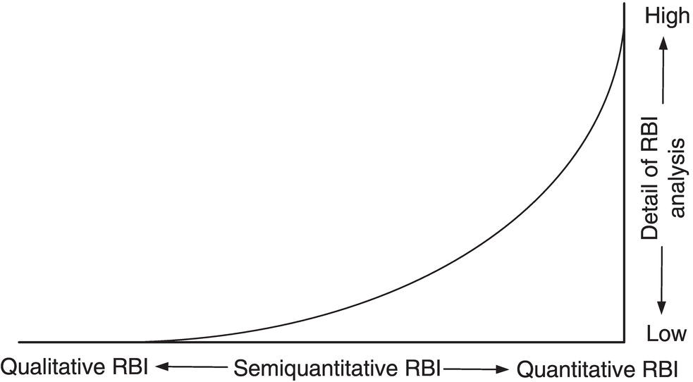
67.2.3 Alternative RBI Approaches
67.2.4 Qualitative Approaches to RBI
67.2.4.1 Probability of Failure Category
67.2.4.2 Consequence of Failure Category
67.2.4.3 Flammable COF Category
67.2.4.4 Health COF Category
67.2.4.5 Business COF Category
67.2.4.6 Final COF Category
67.2.4.7 Qualitative Risk Results
67.2.5 Quantitative RBI Analysis
67.2.5.1 Probability of Failure Analysis

67.2.5.2 Consequence of Failure Analysis
Title
Leadership and administration
Process safety information
Process hazard analysis
Management of change
Operating procedures
Safe work practices
Training
Mechanical integrity
Pre-startup safety review
Emergency response
Incident investigation
Contractors
Audits
67.2.5.3 Estimating the Release Rate
67.2.5.4 Predicting the Type of Outcome
66.7.4.4 Flammable Effects
57.5.3 Toxic Effects
67.2.5.5 Applying Effect Models to Estimate Flammable and Toxic Consequences
57.5.3.2 Environmental Effects
66.7.5 Financial Effects
67.2.5.6 Quantitative Risk Results
67.3 Development of Inspection Programs
67.3.1 Introduction
67.3.2 Inspection Techniques and Effectiveness
67.3.3 Damage Types
67.3.3.1 Inspection Methods
Damage Type
Description
Thinning, general
Uniform loss of material thickness internally and/or externally
Thinning, localized, and pitting
Nonuniform loss of material thickness internally and/or externally
Cracks connected to equipment surface
Cracking at material surface internally and/or externally
Cracking not connected to equipment surface
Cracking in material subsurface, not broken to surface internally and/or externally
Microfissuring/microvoid formation
Small fissures or voids in material subsurface
Metallurgical changes
Changes to the metallurgical microstructure
Dimensional changes
Physical dimension changes
Blistering
Subsurface lamellar blisters at plate inclusions, typically caused by hydrogen diffusion into material
Material properties changes
Changes to the material mechanical properties
Damage Mechanisms
Amine corrosion
CO2 corrosion
Organic chloride corrosion
Organic sulfur corrosion
Microbiological corrosion
Sour water corrosion
Cooling water corrosion
Injection point corrosion
Underdeposit corrosion
Soil corrosion
Atmospheric corrosion
CUI
Cracking Mechanism
Amine cracking
Sulfide stress cracking
HIC/stress-oriented hydrogen-induced cracking (SOHIC)
Damage Mechanism
Damage Types
Sulfide stress cracking
Surface initiated cracking
Hydrogen-induced cracking
Surface and subsurface initiated cracking
Blistering
Subsurface lamellar blisters at plate inclusions
SOHIC
Surface and/or subsurface cracking, cracks can be surface connected
Damage Mechanism
Damage Types
Erosion—solids
Thinning, localized
Erosion—droplets
Thinning, localized
Cavitation
Thinning, localized
Sliding wear
Thinning, general or localized
Fatigue
Surface or sub-surfaced initiated cracking
Corrosion fatigue
Surface initiated cracking
Overload (plastic collapse)
Thinning, localized and dimensional changes
67.3.3.2 Inspection Frequency/Interval
67.3.3.3 Inspection Effectiveness
Inspection Technique
Thinning
Surface Initiated Cracking
Subsurface Cracking
Metallurgical Changes
Dimensional Changes
Blistering
Visual examination
H, M, L
M, L
X
X
H, M, L
H, M, L
Ultrasonic pigging or manual
H, M, L
L, X
L, X
X
X
H, M
Ultrasonic shear wave
X
H, M
H, M
X
X
X
Fluorescent magnetic particle
X
H, M
L, X
X
X
X
Dye penetrant
X
H, M, L
X
X
X
X
Acoustic emission
X
H, M, L
H, M, L
X
X
L, X
Eddy current
H, M
H, M
H, M
X
X
X
Flux leakage
H, M
X
X
X
X
X
Radiography
H, M, L
L, X
L, X
X
H, M
X
Dimensional measurements
H, M, L
X
X
X
H, M
X
Metallography
X
M, L
M, L
H, M
X
X
67.3.3.4 Qualitative Assessment of Inspection Effectiveness
Evaluation Factor
Rigorously Quantitative Approach
RBI Approach
Example of RBI Approach for General Corrosion
Damage density and variability
Density, mean, and extreme value distributions of damage
General corrosion occurs over a substantial portion of the surface area and is relatively uniform
Validity of sample
Sample must be representative of the population about which a statistical inference is to be made
The inspection program is designed to concentrate on areas where damage is likely to occur
For general corrosion, most samples will be representative of the condition; however, the rate of corrosion may vary significantly within one piece of equipment
Sample size
Sample size must be statistically significant
The area inspected should be appropriate for damage mechanisms that are highly localized
Visual examination, combined with ultrasonics, increases the significance of the sample versus spot ultrasonic thickness readings alone
Detection capability
Probability of detection curves describe the capability of the method
The capability of the inspection type is evaluated qualitatively
Visual examination is rated “possibly” to “highly” effective; ultrasonic thickness measurements are rated “moderately” to “highly” effective
Validity of future predictions based on past observations
Damage is modeled showing rate variation with time, and so on
The past observation of damage is used to predict the future, based on increase or decrease in damage rate or based on changes to process parameters affecting damage
General corrosion is assumed to occur at the same rate in the future as in the past, unless the process changes (feedstock, temperature, etc.)
Qualitative Inspection Effectiveness Category
Description of Effectiveness
Highly effective (A)
Inspection methods correctly identify the anticipated in-service damage in nearly every case (80–100%)
Usually effective (B)
The inspection methods will correctly identify the actual damage state most of the time (60–80%)
Fairly effective (C)
The inspection methods will correctly identify the true damage state about half of the time (40–60%)
Poorly effective (D)
The inspection methods will provide little information to correctly identify the true damage state (33–40%)
Ineffective (E)
The inspection method will provide no or almost no information that will correctly identify the true damage state (33%)
67.3.3.5 Quantifying Inspection Effectiveness
67.3.4 Probability of Detection
67.3.5 Reducing Risk through Inspection
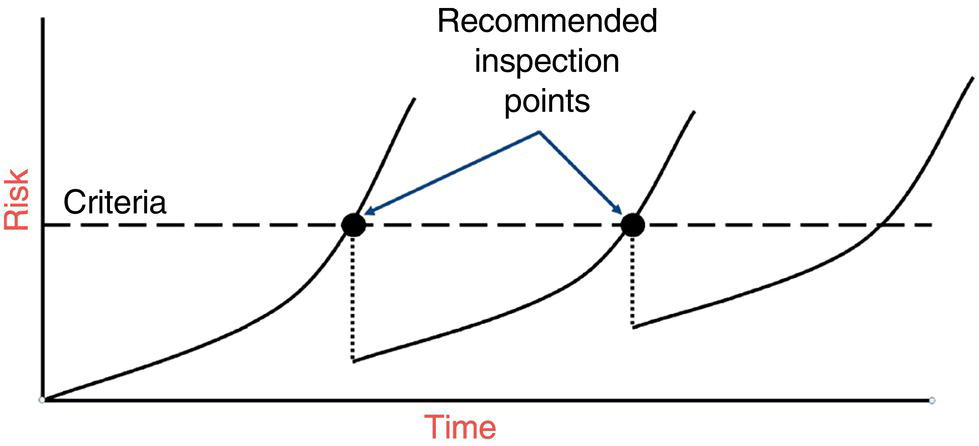

67.4 Putting RBI Into Practice
67.4.1 A Continuum of Approach
67.4.2 Qualitative Versus Quantitative Examples
Equipment type:
Drum
Material of construction:
Carbon steel
Fabrication date:
8/2001
Diameter:
36 in.
Height:
7 ft.
Furnished thickness:
0.375 in.
tmin:
0.285 in.
Corrosion allowance:
0.090
Insulation:
Yes
PWHT:
No
Process stream composition:
12% C1; 22% C2; 24% C3; 21% C4; 13% C5+; 2.8% CO2; 5% H2O; 2000 ppm H2S
Phase:
Gas
Operating pressure:
180 psi
Operating temperature:
104 °F
Expected corrosion rate, internal thinning:
10 mpy
Expected corrosion rate, corrosion under insulation (CUI) thinning:
10 mpy
H2S damage susceptibility:
Medium
Inspection history:
B level 2006
B level 2010
B level 2013
Next planned inspection:
B level 2017
67.4.3 Qualitative Example
67.4.3.1 POF Category
POF Category
Rate of Damage
COF Category
1
2
3
4
4
CR ≥10 mpy
9
5
3
2
3
CR 5–10 mpy
10
8
5
4
2
CR 2–≤5 mpy
10
10
8
6
1
CR ≤2 mpy
10
10
10
9
LOF Category
Cracking Susceptibility
COF Category
1
2
3
4
4
High
10
10
5
2
3
Medium
10
10
7
4
2
Low
15
15
10
6
1
None
–
–
–
–
67.4.3.2 COF Category
67.4.3.3 Risk Results
Analysis
Basis
Results COF Category
COF
Flammable
4
Health
3
Final
4
POF category
POF
Thinning, 10 pmy
4
Thinning, 5 mpy
2
Cracking
3
Risk category
Risk
Thinning, 10 mpy
High
Thinning, 5 mpy
Medium-high
Cracking
High frequency
Inspection planning
Thinning, 10 mpy
2
Thinning, 5 mpy
6
Thinning, 5 mpy RL
0.3
Cracking
4
API Fluid Name
Applicable Materials
COF, Flammable
COF, Toxic
C1–C2
Methane, ethane, ethylene, LNG, fuel gas
4
0
C3–C4
Propane, butane, isobutane, LPG
4
0
C5
Pentane
3
0
C6–C8
Gasoline, naphtha, LSR, heptane
3
0
C9–C12
Jet fuel. Light kerosene
3
0
C13–C16
Diesel, heavy kerosene, Atm gas oil
3
0
C17–C25
Gas oil, crude
2
0
C25+
Residuum, heavy crude
2
0
Water
Water
l
0
Steam
Steam
l
0
Acid-LP
Low pressure acid/caustic
3
0
Acid-MP
Medium pressure acid/caustic
3
0
Acid-HP
High pressure acid/caustic
3
0
H2
Hydrogen only
3
0
H2S
Hydrogen sulfide
3
4
HF
Hydrofluoric acid
0
4
Aromatics
Benzene, toluene, xylene, cumene
3
0
Ammonia
Ammonia
0
4
HCl
Hydrochloric acid
0
5
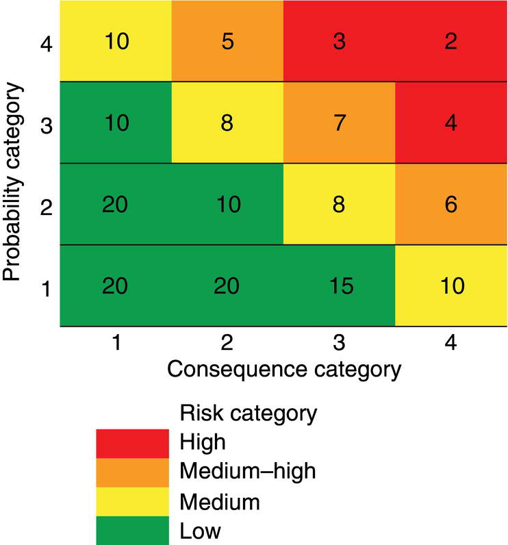
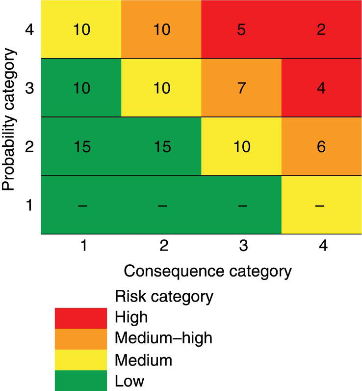
67.4.3.4 Inspection Planning
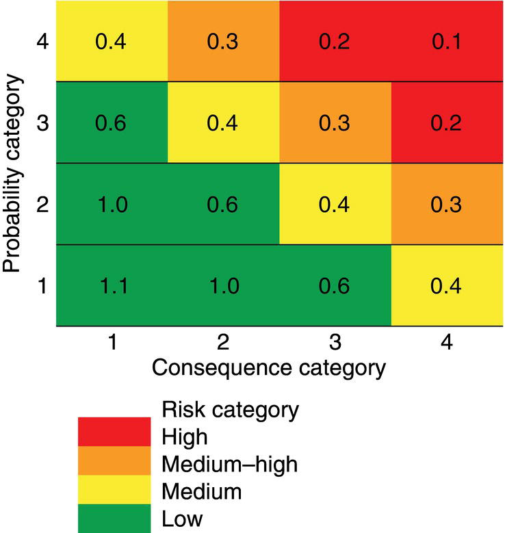
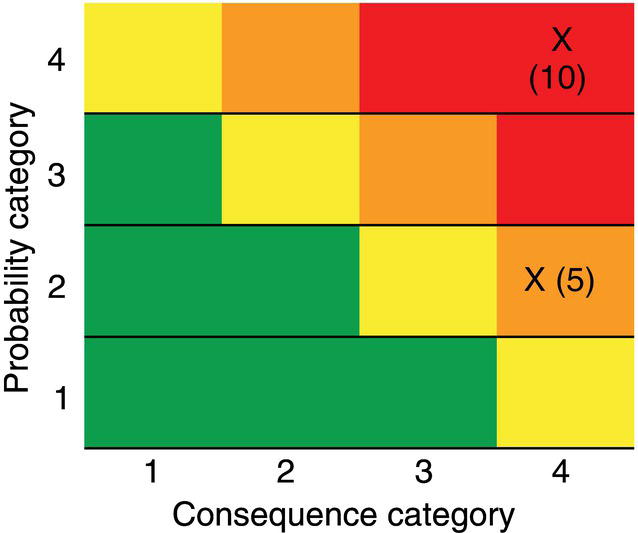
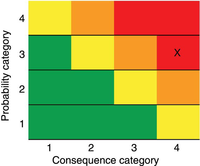
67.4.4 Quantitative Example
67.4.4.1 POF Calculation
Age
Corrosion Rate
(ar/t)
DF, No Inspection
No. of B Inspections
DF
Thinning POF Category
5
0.01
0.13
90
0
90
3
5
0.005
0.07
1
1
1
1
9
0.005
0.12
6
1
2
1
9
0.005
0.12
6
2
1
1
13
0.005
0.17
170
2
7
2
13
0.005
0.17
170
3
2
1
17
0.005
0.23
400
3
6
2
17
0.005
0.23
400
4
2
1

Age
Susceptibility
No. of C Inspection
DF
Cracking POF Category
5
Medium
0
58.75
3
9
Medium
0
112.1
1
13
Medium
0
168.0
1
17
Medium
1
1
2
17
Medium
1
33.50
1
Year
Age
Thinning DF
Cracking DF
Combined DF
FMS
Gff
POF
POF Category
2001
5
90
58.73
167.73
1
1.56E−05
2.32E−03
4
2006
5
1
58.73
59.73
1
1.56E−05
9.32E−04
3
2010
9
2
112.12
114.12
1
1.56E−05
1.78E−03
4
2010
9
1
112.12
113.12
1
1.56E−05
1.76E−03
4
2013
13
7
168.01
175.01
1
1.56E−05
2.73E−03
4
2013
13
2
168.01
170.01
1
1.56E−05
2.65E−03
4
2017
17
6
225.68
231.68
1
1.56E−05
3.61E−03
4
2017
17
2
1.00
3.00
1
1.56E−05
4.68E−05
1
67.4.4.2 COF Category
Analysis
Basis
Results
COF Area
COF Category
COF
Flammable, equipment
943.66
B
Flammable, injury
2443.84
C
Toxic
226.84
B
Final
2443.84
C
Category
Probability Category
Consequence Category
POF Range
DF Range
Category
Range (ft2)
1
POF ≤ 1.00E−04
DF ≤ 1
A
CA ≤ 100
2
1.00E−04 < POF ≤ 1.00E−03
1 < DF ≤ 10
B
100 < CA ≤ 1000
3
1.00E−03 < POF ≤ 1.00E−02
10 < DF ≤ 100
C
1000 < CA ≤ 10,000
4
1.00E−02 < POF ≤ 1.00E−01
100 < DF ≤ 1000
D
10,000 < CA ≤ 100,000
5
POF > 1.00E−01
DF > 1000
E
CA > 100,000
67.4.4.3 Risk Results
Analysis
Basis
Results
COF Area
COF Category
COF
Flammable, equipment
943.66
B
Flammable, injury
2,443.84
C
Toxic
226.84
B
Final
2443.84
C
DF/Risk
POF Category
POF at 2017
Thinning
6
2
Cracking
225.68
4
Total
231.68
4
POF
3.61E−03
4
Risk
Total
Risk Value, ft2/year
Risk Category 4C—high
8.83
Inspection Planning risk after inspection
Thinning—1B
2
1
Cracking—1C
1
1
Total DF
3
2
POF
4.68E−05
2
Risk
Risk Value, ft2/year
Risk Category
1.14E−01
2C—low
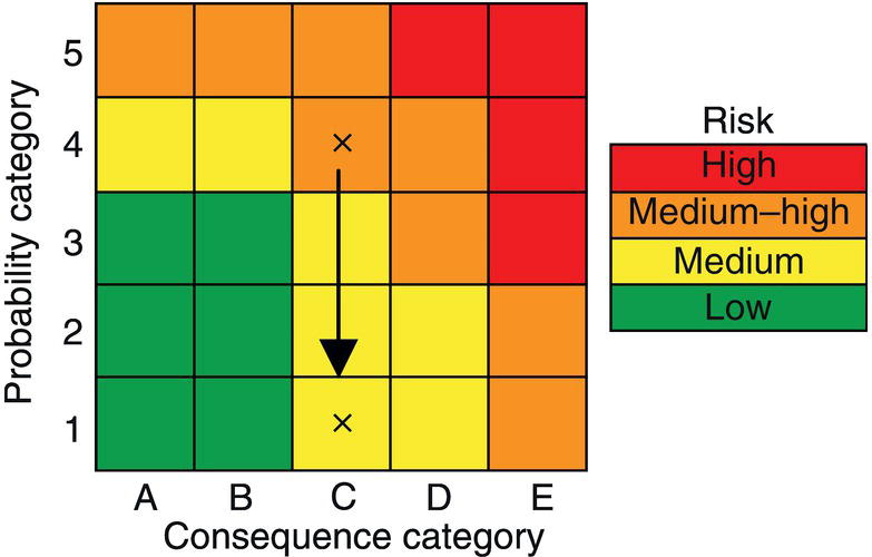
67.4.4.4 Inspection Planning
67.4.5 Optimizing the Inspection Program
67.4.6 Example Problem Conclusions
67.4.6.1 Qualitative RBI Characteristics
67.4.6.2 Quantitative RBI Characteristics
67.5 Conclusion: Evaluating RBI Methodologies
67.5.1 Summary
67.5.2 Ten Criteria for Selecting the Most Appropriate Level of RBI
67.5.3 Justifying Costs
References
Bibliography
Note