52.1 Introduction

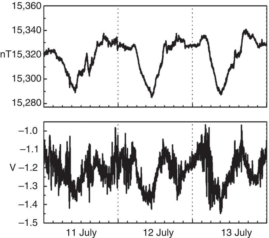
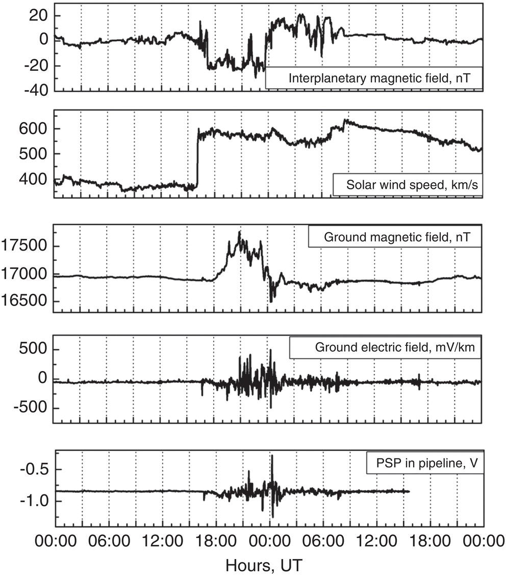
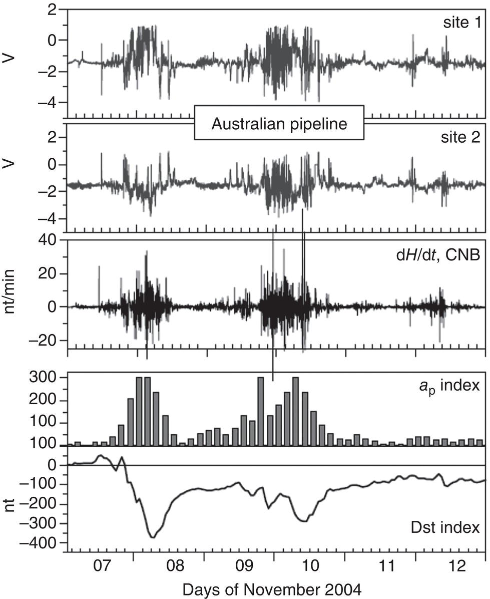
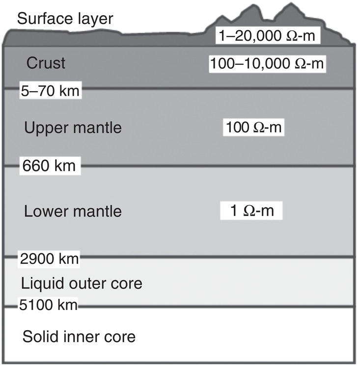
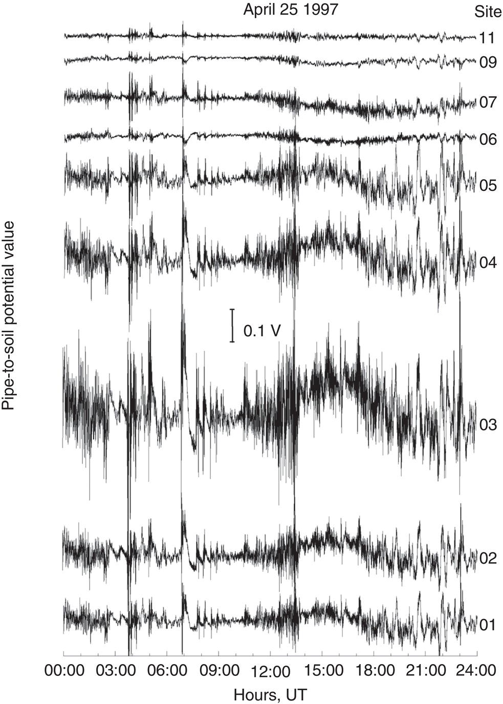
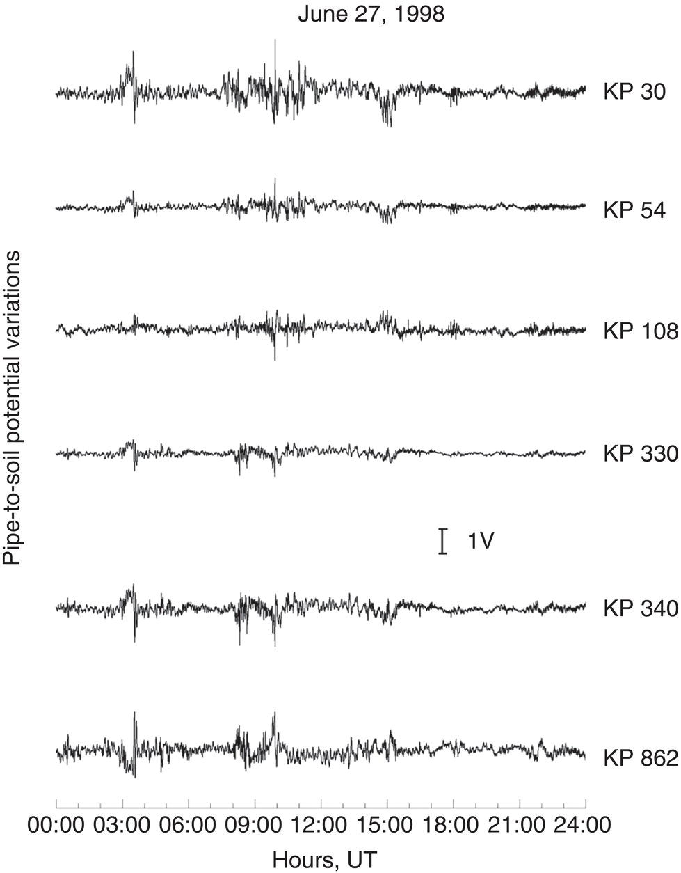
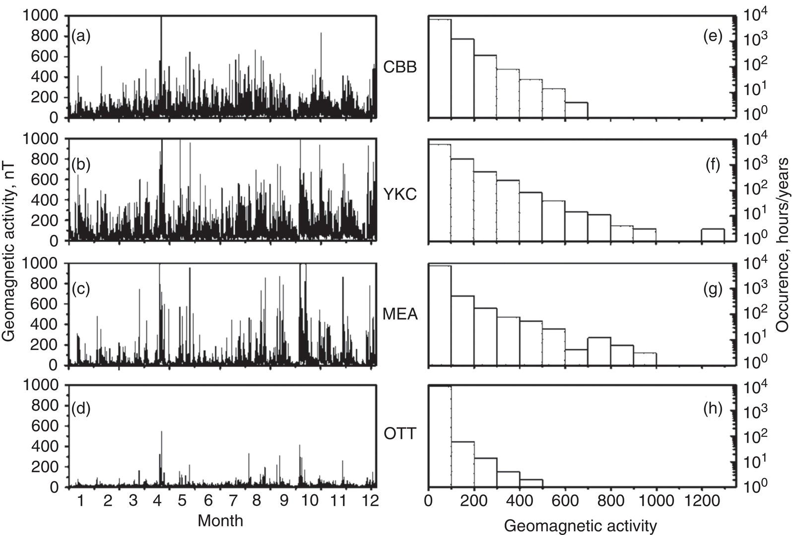
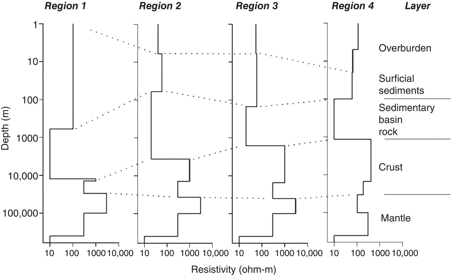
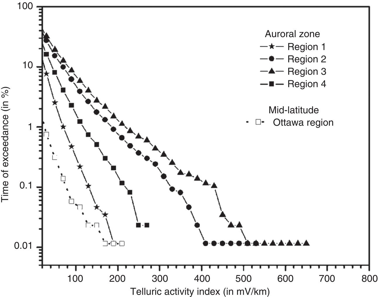
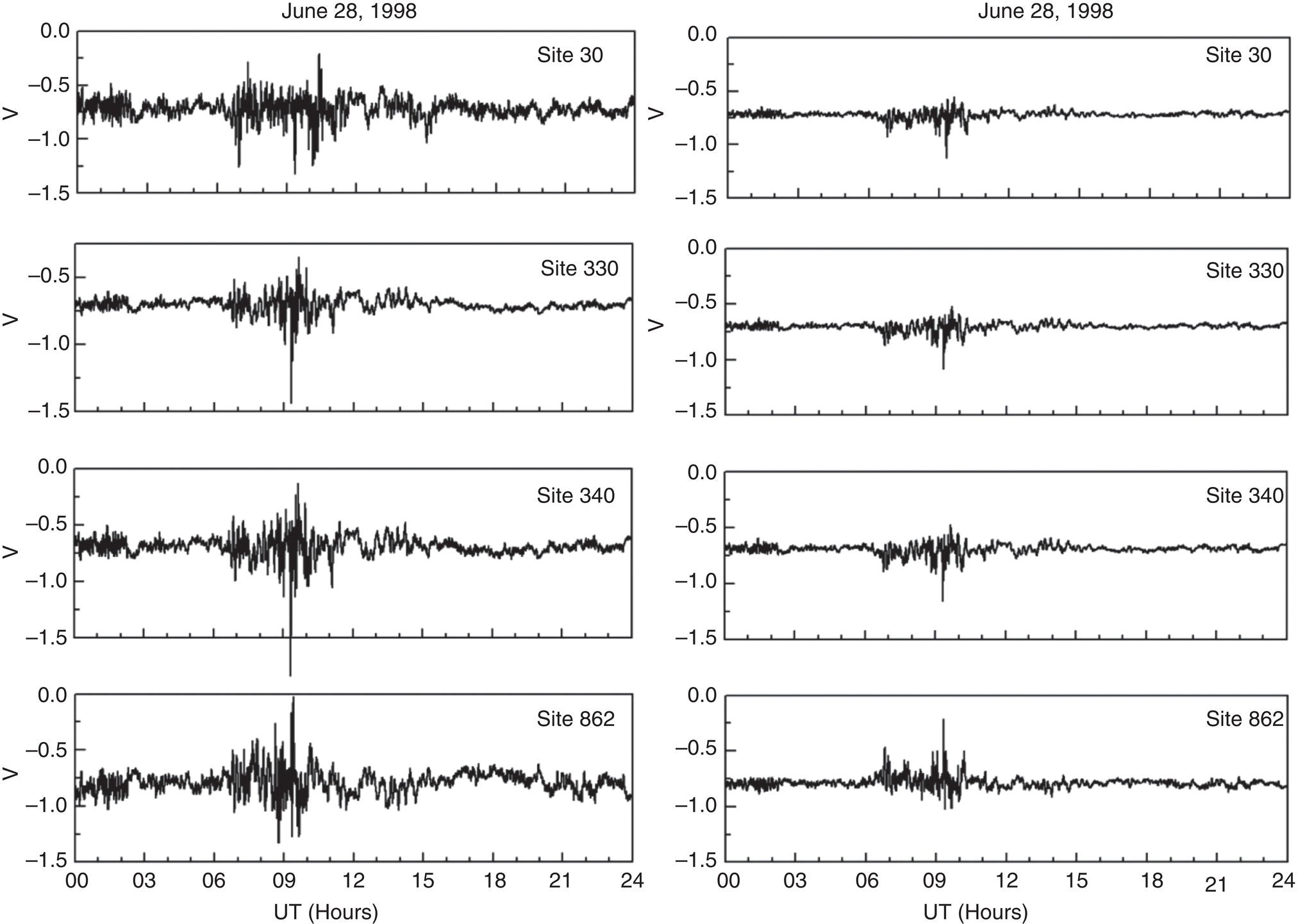
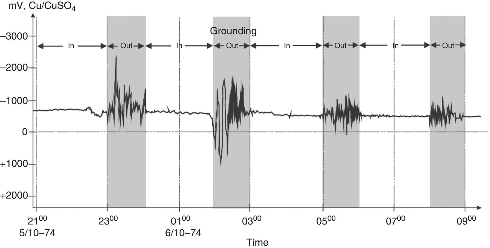
Telluric currents are the electric currents produced in the ground by natural geomagnetic field variations. One of the first experiments to record telluric currents was carried out in 1862 [1]. The currents and corresponding electric fields are primarily induced by changes in the Earth’s magnetic field, which are usually caused by interactions of the solar disturbances propagating and impacting the Earth’s natural electromagnetic environment. Recordings of these magnetic field variations and electric fields have been widely used since the 1950s for mineral exploration [2].

In pipelines, telluric currents are responsible for variations in pipe-to-soil potentials (PSPs) that interfere with pipeline surveys and might contribute to pipeline corrosion [3] [4, 5]. Evaluating the telluric influence on a pipeline is difficult due to its irregular nature. This is nicely described by Shapka [6]:

Pipeline potentials would remain unchanged for several weeks, then begin fluctuating anywhere from 100 millivolts to 15 volts. Further investigation showed that these disturbances correlated closely to variations in the Earth’s magnetic field.

Telluric variations have a continuous frequency spectrum, as distinct from single frequency variations due to alternating current (AC) interference. Also, PSP variations due to tellurics are different for different locations along the pipeline, which can be confusing when doing a close-interval pipeline survey.

To help understand all these features of telluric currents, this chapter provides a review of the literature followed by an explanation of the geomagnetic sources of telluric activity, the impacts of Earth’s deep conductivity structures, a pipeline’s response to telluric electric fields and the methodology for assessing telluric effects, and mitigation/compensation of telluric effects. To conclude, we examine the knowledge gaps and open questions about telluric effects.

52.2 Review of the Existing Knowledge on Pipeline-Telluric Interference

The first report of telluric currents in pipelines comes from Varley in 1873, who commented that currents on a telegraph cable in London appeared to be associated with telluric currents in nearby gas pipelines [7, 8]. However, studies focused on telluric current effects on pipelines have been reported for just over half a century. Early work on an 1128-mile pipeline in Canada noted the existence of stray currents that could not be accounted for by any of the usual sources and indicated a possible association with magnetic disturbances [9]. The variations of PSP or currents along the pipeline associated with telluric activity have been reported from nearly every part of the world, for example, New Zealand [10–12], Africa [13], Australia [14–17], Europe [18–31], the USA [32–41], Argentina [42–45], and Canada [46–48] and not only on pipelines buried in the ground but on the seafloor as well [49].

The telluric influence has represented an ongoing problem for engineers setting up cathodic protection systems, and the variations in PSP produced by telluric currents often make pipeline surveys difficult [10, 36, 50]. The most significant telluric currents are associated with large geomagnetic disturbances [51, 52], although tidally induced effects have also been reported [12]. Early attempts to suppress the telluric currents effects include the pipeline grounding, investigated in Norway [53]. Later observations in Northern Canada by Seager showed how the amplitude of telluric PSP fluctuations is affected by the introduction of an insulating flange into the pipeline [54]. Experimental techniques have also been developed for correcting close-interval potential surveys [40, 55, 56] and pipeline test station surveys [57], although they can require knowledge of telluric effects to use them appropriately [58].

Construction of the Alaska pipeline in the high-latitude region noted for enhanced geomagnetic and telluric activity prompted more dedicated quantitative studies and numerical modeling. For the Alaska pipeline, Campbell [59] calculated the telluric currents that could be produced in the pipeline and their dependence on geophysical parameters such as the Earth’s conductivity structure and frequency spectrum of the geomagnetic disturbances. Numerical modeling of the effects of telluric currents on pipelines has also been made for pipelines in Finland [27], Argentina [60], and Nigeria [61]. All the aforementioned modeling has been done based on the assumption that the pipeline is a single infinitely long conductor. The inclusion of the coating properties was made by modeling the pipeline as multiple concentric cylinders [62, 63]. Pirjola and Lehtinen [64] modeled a single pipeline with discrete ground connections. The modeling was extended to include the continuous high-resistance connection to ground through a pipeline coating by the application of distributed source transmission line theory. This was based on the methods developed for AC interference [65–68], adapted for telluric modeling [69–71], and continues to be the most widely used method due to its versatility [47, 72–78].

The development of numerical modeling of telluric effects on pipelines has provided the theoretical foundation for understanding the telluric observations and provided tools to aid in the design of cathodic protection systems [79–81]. Telluric influence is now often considered part of the pipeline design process [82–84]. Further explanations of the methodology for assessing telluric effects on a pipeline are presented in the section on mitigation.

Greater awareness of telluric effects has prompted several large-scale investigations, such as the simultaneous measurements of the telluric variations of the PSPs in multiple locations along a pipeline made in different countries [85], as well as the detailed Pipeline Research Council International review of the existing knowledge on the telluric interference with pipelines [86].

Telluric effects on pipelines are part of a wider field of geomagnetic effects on ground infrastructure [8, 87–90] that dates back to the 19th century and the early days of the telegraph [91]. In a major magnetic storm in 1859, telegraph services around the world were disrupted with many accounts of messages being interrupted during the disturbance [92]. Subsequent telluric disturbances produced problems and in 1921 telluric currents started fires at several telegraph stations in Sweden [93]. As technology changed, telluric effects were observed on other systems. Submarine phone cables were affected [94], and a major storm on August 4, 1972, produced an outage of the L-4 phone cable system in the Midwestern United States [95]. Telluric currents also occur in power systems, where they are referred to as geomagnetically induced currents (GIC). The GIC induced in transmission lines flow to ground at substations causing saturation of power transformers leading to a variety of problems with power system operation [96, 97]. On March 13, 1989, one of the biggest magnetic storms of the last century sent electric currents surging through power systems in North America and Northern Europe [98]. The result was equipment and lines tripped out of service, burnt-out transformers, and the collapse of the Hydro-Québec power system, leaving the 6 million residents of Québec without power for over nine hours [99]. This all has stimulated research into the impacts of natural electromagnetic environment on ground infrastructure and has significantly contributed to advancing our understanding of telluric effects on pipelines [100–104].

52.3 Geomagnetic Sources of Telluric Activity

The geomagnetic field variations that produce telluric activity have their origin in processes on the Sun [105]. The electromagnetic and particle radiation from the Sun affects the Earth’s magnetic environment in a variety of ways [106]. Regular electromagnetic radiation (light) heats the dayside part of the Earth’s atmosphere, producing vertical convection that drives electric currents in the ionosphere (conductive top layer of the Earth’s atmosphere). These electric currents create a magnetic field on the dayside of the Earth that is superimposed on the Earth’s internally generated magnetic field. A site on the Earth’s surface is carried by the Earth’s rotation into this extra magnetic field in the morning and out again in the evening. This produces the normal magnetic field variation seen on quiet days. Figure 52.1 shows an example of the geomagnetic diurnal variation in Norway and simultaneous recordings of PSP on a nearby pipeline [26].

Irregular periods of solar activity produce disturbances such as coronal mass ejections (CMEs) and high-speed streams that travel from the Sun through interplanetary space (solar wind) to the Earth. These disturbances interact with the Earth’s magnetic field, creating geomagnetic storms that enhance telluric currents. Figure 52.2 shows an example of a solar disturbance reaching the Earth, seen by the sudden changes in the interplanetary magnetic field and the solar wind speed in the top two panels. The next two panels show the magnetic disturbance and telluric electric field observed on the ground. The bottom panel shows recordings of the resulting PSP variations on a pipeline.

The sizes of geomagnetic field variations associated with particular types of solar phenomena are not the same all over the Earth. The diurnal variation is largest near the equator, where the currents driven by solar heating are greatest and decrease slowly with increasing latitude. In contrast, the irregular geomagnetic field variations and geomagnetic storms produced by high-speed streams and CMEs are most intense at high latitudes (above 65°). It should be noted that the same processes that give rise to the geomagnetic disturbances also produce the aurora, and the “auroral zone,” the region where the aurora is most frequently seen, is also a region of high telluric activity. Mid-latitudes will experience a mixture of these auroral and equatorial disturbances. Early accounts of telluric activity were generally from high-latitude pipelines, but the use of higher resistance coatings on modern pipelines (see Section 52.6.3) has increased the amplitude of telluric PSP fluctuations and means that they can now be seen on pipelines at any latitude.

Figure 52.3 shows an example of PSP recordings made on an Australian pipeline during a geomagnetic disturbance [107]. Ap and Dst are global geomagnetic activity indices showing the worldwide level of disturbance in the geomagnetic field. The middle panel shows the rate of change of the magnetic field, dH/dt, recorded at Canberra, the magnetic observatory closest to the pipeline location. It can be seen that the size of these variations follows the general trend of the global activity indices. The PSP variations at two sites on a nearby pipeline are closely related to the rate of change of the local magnetic field.

Thus, in understanding the influence of telluric currents on PSP variations, it is important to compare these variations with nearby geomagnetic recordings if available or with the variations of the global geomagnetic activity [74, 108, 109].

52.4 Earth Resistivity Influence on Telluric Activity

The size of telluric electric fields produced by the geomagnetic field variations depends on the rate of change of the magnetic field variations and the deep earth resistivity structure of the region traversed by the pipeline [2, 74]. Geomagnetic field variations at low frequencies (mHz) penetrate tens to hundreds of kilometers into the Earth, and the resistivity down to these depths needs to be taken into account to calculate the electric fields at the Earth’s surface.

The Earth is comprised of a number of layers, as shown schematically in Figure 52.4. At the Earth’s surface the resistivity depends on the rock type with sedimentary rocks being less resistive than granitic igneous rocks. Below the surface layer, the crust of the Earth is resistive but at greater depths the increasing temperature and pressure causes a decrease in resistivity.

Higher resistivities cause larger telluric electric fields to be produced during geomagnetic disturbances, while the lower resistivity rocks have lower telluric electric field values. Thus, a pipeline passing through regions with different resistivities will experience larger telluric currents in the region with the higher resistivity [44, 60]. Changes in soil resistivity at the surface can also affect the discharge of telluric currents from a pipeline [40].

Boundaries between regions of different resistivity, such as at the interface between geological terrains, also produce localized enhancements of the electric fields that can affect pipelines [26, 45, 110–112]. For example, Figure 52.5 shows the changes in amplitude of PSP variations at sites along a 150 km stretch of pipeline. These could not be explained by the pipeline structure but coincided with earth resistivity changes associated with a geological boundary [85]. The resistivity boundary effect is also significant at a coastline because of the large contrast between the resistivity of the land (100–10,000 ohm-m) and seawater (0.25 ohm-m) [86, 113].

52.5 Pipeline Response to Telluric Electric Fields

The telluric electric fields produced by geomagnetic field variations will drive telluric currents along a pipeline as well as in the ground. The “potential drop” produced by these currents flowing on and off the pipeline is the cause of the telluric PSP variations. During the course of a geomagnetic disturbance, the telluric electric field will reverse direction many times causing a similar change in the direction of the telluric current resulting in many fluctuations of the PSP on the pipeline, as shown in Figure 52.6 [85]. It shows that the PSP variations at the southern end (KP 862) of the pipeline are out of phase (oppositely directed) from the PSP variations in the northern part of the pipeline, consistent with the telluric currents generally flowing on and off the pipeline at opposite ends.

The size of PSP variations produced by telluric currents flowing on and off a pipeline depends on the resistance to ground from the pipeline steel. In the absence of any ground beds, this is determined by the resistance through the pipeline coating: the more resistive the coating, the larger the telluric PSP fluctuations that are produced. In fact, it is the trend over the last 40 years for the use of higher resistance coatings that has caused telluric PSP variations to be larger on modern pipelines. The amplitude of the PSP fluctuation generally decreases with distance from the end of the pipeline. This falloff is characterized by the “adjustment distance” determined by the resistance along the pipeline steel and the conductance through the coating to the ground and typically has values of many tens of kilometers [69]. The decrease in coating conductance has not only increased the size of the telluric PSP fluctuations but has also increased the adjustment distance, meaning that sizeable telluric PSP fluctuations are seen further along the pipeline.

In practice, many specific things about the pipeline structure or the electric fields can affect the telluric current flow along the pipeline, affecting the size and location of the telluric PSP fluctuations that occur. If an insulating flange is inserted into the pipeline, it effectively creates new endpoints where the telluric current flows on or off the pipeline, thus creating extra sites where telluric PSP fluctuations occur. In fact, any pipeline feature that alters the flow of telluric currents along the pipeline will give rise to the currents flowing on or off the pipeline, producing the associated telluric PSP fluctuations. Changes in direction (bends) of a pipeline or changes from one to two pipelines (such as sometimes occurs at a compressor station on a gas pipeline) are places where larger telluric PSP fluctuations may occur [114].

52.6 Telluric Hazard Assessment

The size of telluric PSP variations produced during a geomagnetic disturbance depends on (1) the amplitude of the geomagnetic field variations, (2) the conductivity structure of the Earth, and (3) the pipeline response, as already discussed. Assessing the telluric hazard to a pipeline requires knowledge about all three factors.

52.6.1 Geomagnetic Activity

Geomagnetic disturbances come in many sizes, with many small ones, a lesser number of medium disturbances, and a few very large disturbances. A good guide to the geomagnetic activity to which a pipeline will be exposed in the future can be provided by analyzing a representative sample of past activity. Recordings of geomagnetic disturbances are made at magnetic observatories around the world, and data back to 1991 are available from Intermagnet (www.intermagnet.org). (Earlier data may also be obtained by contacting the institutes operating the magnetic observatories.) By analyzing data from an observatory in the vicinity of a pipeline, it is possible to determine the rate of occurrence of different levels of geomagnetic activity that will be experienced by the pipeline.

As an example, the results of the statistical analysis made of the magnetic activity in different latitudinal zones of Canada represented by data from four geomagnetic observatories for the year 2002 [115] are presented in Figure 52.7. Observatories at Cambridge Bay (CBB), Yellowknife (YKC), and Meanook (MEA) are located in the auroral zone, and Ottawa (OTT) in the subauroral zone. The range of the magnetic field variations in each hour is used as a measure of the size of the geomagnetic activity. Figures 52.7a–d show the variations of hourly range values (in nanoTesla) during the year, while Figure 52.7e–h show the number of hours per year with different levels of geomagnetic activity.

52.6.3 Pipeline Response

The next step of the assessment process is the modeling of the pipeline. This can be done in a manner similar to that used for studying AC induction in pipelines [65–68]. Each pipeline section is defined by its electrical properties (series impedance along the pipeline determined by the resistivity and cross-sectional area of the pipeline steel and parallel admittance given by the conductance (1/resistance) to ground through the pipeline coating) [69]. The telluric electric field is represented by a voltage source in each section. Multiple pipeline sections can be combined using a network modeling approach to provide models for a complete pipeline network [71, 78].

The calculated electric fields are then used as inputs to the model to obtain the PSP across the pipeline. Figure 52.10 shows recordings of PSP variations on a pipeline produced by telluric currents (left panel) and modeled using a calculated telluric electric field and a model of the pipeline [74].

These results demonstrate where in the pipeline network the largest telluric PSP will occur and combined with the E-field statistics of Figure 52.9, can show how often specific PSP levels will be exceeded. This provides the pipeline designer/operator with information about the telluric influence on the pipeline and can be used to examine mitigation options if required.

52.7 Mitigation/Compensation of Telluric Effects

NACE¹ Report “CEA 54276” in 1988 says

Telluric effects can give rise to large fluctuations in measured potential values, sometimes of the order of several volts positive or negative. In such cases […] specialist advice is sought either to monitor and suitably correct the measured values or to choose a survey period when geomagnetic activity is at a minimum.

Views on the most appropriate action to take to mitigate telluric effects have evolved over time as understanding has improved. An early suggestion for mitigation of telluric effects was to install insulating flanges to block the flow of currents along the pipeline [36]. However, as illustrated in Figure 52.11, it is now recognized that disrupting the telluric current flow along the pipeline forces it to flow through the coating to ground, increasing the PSP variations for the pipeline on either side of the flange.

The strategy adopted in the last 20 years is to remove obstacles to the flow of telluric currents by removing or jumpering around insulating flanges and providing good connections to ground, that is, a path for telluric currents to easily flow on and off the pipeline without passing through the pipeline coating. As well, ground beds are also placed at other places along the pipeline, such as bends [4, 86]. The effect of good grounding on reducing telluric PSP variations can be seen in Figure 52.12.

Another strategy is to use potential-controlled rectifiers, as shown in Figure 52.13 [46, 80]. Here, the pipeline modeling can be useful in determining the range of variations that must be controlled. Information from the modeling about where the telluric fluctuations change sign should also be used to guide placement of potential-controlled rectifiers otherwise there is a danger that telluric compensation in one part of a pipeline may “overflow” into a neighboring part where it would actually increase the PSP variations.

Telluric fluctuations in pipelines may make it difficult to obtain reliable potential survey data. In some cases, it may be sufficient to wait for geomagnetic quiet times to conduct pipeline surveys. (Long-term forecasts of geomagnetic activity can help with survey planning.) However, in other cases, it can be necessary to take active steps to compensate the survey data for telluric effects. This has been done by using a reference site to provide a telluric level that can be subtracted from the survey data [58, 117]. For the Alaska pipeline measurements of the telluric current along the pipeline were used [57], again with the purpose of subtracting off the telluric fluctuations in the survey data. Finally, online model calculations can be made using geomagnetic data to calculate the telluric PSP variations occurring during the time of a survey [116, 118].

52.8 Knowledge Gaps/Open Questions

Above, we have shown the methodology for assessing the telluric hazard to a pipeline, but this needs the appropriate input data: for example, geomagnetic data and earth conductivity structure. Geomagnetic data are available from many magnetic observatories around the world (see www.intermagnet.org). The proximity of an observatory to a pipeline varies considerably. Even in places such as North America with reasonably good coverage of magnetic observatories, the observatory recordings may not be sufficient to map the changes in magnetic activity along a pipeline route. In such cases, temporary installation of magnetometers along the pipeline route could be considered.

Earth conductivity models to use for the electric field calculations can be constructed from magnetotelluric survey results published in the geophysical literature. Such earth models are also required for studies of geomagnetic effects on power systems and this has led to the production of compendiums of earth models that can be used for both pipeline and power system studies [119, 120]. These earth models are one-dimensional models; that is, they only account for the variation of conductivity with depth, while, as mentioned earlier, lateral variations in conductivity also influence the electric fields experienced by pipelines. The study of such effects requires the use of two- or three-dimensional modeling techniques [121].

Telluric PSP variations are a concern both because of the impacts on the PSP recordings, which make it difficult to identify the real reason for PSP anomalies, and because of their possible contribution to corrosion [4, 5]. There are definitely not enough measurements done of the corrosion rates due to the telluric activity [29, 30], which makes it difficult to evaluate the contribution of telluric activity in the overall corrosion process. Like other stray currents, the variable nature of the telluric shifts of PSP will produce less effect on corrosion rates than a direct current (DC) shift [122, 123]. In this regard, their effect may be similar to AC corrosion. Chapter 60 on AC corrosion states that it is necessary to understand the interplay of the AC and DC levels on the pipeline in order to assess the corrosion rates. Similar investigations need to be undertaken for telluric activity.

52.9 Summary

Telluric PSP variations have been observed on pipelines in many parts of the world and are a concern because of interference to pipeline surveys and for creating conditions that may contribute to corrosion of the pipeline.

The telluric activity originates from the activity on the Sun that causes geomagnetic disturbances on the Earth. The telluric electric fields enhanced due to these disturbances depend on the amplitude and frequency content of the geomagnetic field variations and on the deep earth conductivity structure.

Pipeline response to telluric electric fields is controlled by the electrical properties of the pipeline: the series impedance of the steel and the parallel admittance through the coating. Use of higher resistance coatings on modern pipelines has increased the size of telluric PSP variations that occur making telluric effects visible on pipelines all over the world.

If telluric influence is suspected on a pipeline then a telluric hazard assessment can be made taking account of the geomagnetic activity, earth structure, and pipeline characteristics to determine how often specified PSP levels will be exceeded in different parts of the pipeline.

Mitigation now focuses on allowing telluric currents to flow along the pipeline and providing good ground connections to drain currents off the pipeline at the ends, bends, and so on. Comparison with reference recordings can be used to correct survey data.

Substantial work is required to properly evaluate the impact of telluric PSP fluctuations on pipeline corrosion and possible disbondment of coatings.

Acknowledgments

The authors have benefitted from many useful discussions with R.A. Gummow. Funding from the Panel for Energy Research and Development (PERD) has contributed to a number of studies that have helped to develop the understanding of telluric currents.

References

1. 1 Lamont, J.V. (1862) Der Erdstrom und der Zusammen desselben mit dem Erdmagnetismus, Leopold-Voss-Verlag, Leipzig und Muenchen.
   
2. 2 Kaufman, A.A. and Keller, G.V. (1981) The Magnetotelluric Sounding Method, Methods in Geochemistry and Geophysics, Elsevier, Amsterdam, Vol. 15, p. 595.
   
3. 3 Peabody, A.W. (2001) Peabody’s Control of Pipeline Corrosion, 2nd ed., NACE International, Houston, TX.
   
4. 4 Gummow, R.A. (2002) GIC effects on pipeline corrosion and corrosion control systems. Journal of Atmospheric and Solar – Terrestrial Physics, 64, 1755–1764.
   
5. 5 Trichtchenko, L., Trishchenko, A.P., Hejda, P., and Langer, R. (2023) Evaluation of telluric-associated corrosion on buried pipelines, Journal of Atmospheric and Solar-Terrestrial Physics 248, 106082. doi: https://doi.org/10.1016/j.jastp.2023.106082.
   
6. 6 Shapka, R.S. (1993) Geomagnetic effects on a modern pipeline system. Proceedings Solar-Terrestrial Predictions Workshop, May 18–22, Vol 1, 1993, Ottawa, Canada. pp. 163–170.
   
7. 7 Varley, C.F. (1873) Discussion of a few papers on Earth currents. Journal of the Society of Telegraph Engineers, 2, 111–114.
   
8. 8 Lanzerotti, L.J. and Gregori, G.P. (1986) Telluric currents: the natural environment and interactions with man-made systems. In: The Earth’s Electrical Environment, National Academy Press, Washington, DC, pp. 232–257.
   
9. 9 Allison, N.J. and Huddleston, W.M.E. (1952) Extraneous currents noted on large transmission pipe line system. Corrosion, 8(1), 1.
   
10. 10 Procter, T.G. (1974) Experience with telluric current interference in the cathodic protection of a buried pipeline in New Zealand. Materials Performance, 13(6), 24.
    
11. 11 Procter, T.G. (1975) Pipeline telluric current interference as one phase of a wider interdisciplinary technological problem. Materials Performance, 14(8), 24–28.
    
12. 12 Boteler, D.H. and Cookson, M.J. (1986) Telluric currents and their effects on pipelines in the Cook Strait region of New Zealand. Materials Performance, 25(3), 27–32.
    
13. 13 Barker, R.H. and Skinner, N.J. (1980) The flow of electric currents of telluric origin in a long metal pipeline and their effect in relation to corrosion control. Materials Performance, 19(2), 25–28.
    
14. 14 McCoy, J. (1989) Cathodic protection on the Dampier to Perth pipeline—Australia. Materials Performance, 28(2), 16–20.
    
15. 15 Martin, B.A. (1993) Telluric effects on a buried pipeline. Corrosion, 49(4), 343–350.
    
16. 16 Martin, B.A. (1993) Telluric effects on an equatorial pipeline in Papua New Guinea. Proceedings of the Australasian Corrosion Association Conference 33, Paper No. 40, November, 1993.
    
17. 17 Martin, B.A. (1994) Cathodic protection of a remote river pipeline. Materials Performance, 33(3), 12–15.
    
18. 18 Brooks, D.R. (1983) Responding to the challenge in engineering. Gas Engineering and Management, 23, 355–367.
    
19. 19 Brasse, H. and Junge, A. (1984) The influence of geomagnetic variations on pipelines and an application for large-scale magnetotelluric depth sounding. Journal of Geophysics, 55, 31–36.
    
20. 20 Camitz, G., Edwall, H.-E., and Marbe, A. (1997) The influence of telluric currents on the cathodic protection of natural gas pipelines. Proceedings of the CEOCOR 4th International Conference, 1997, Sector A, Vienna, Austria. pp. 125–135.
    
21. 21 Edwall, H.-E. and Boteler, D. (2001) Studies of telluric currents on pipelines in Southern Sweden. Proceedings, CORROSION 2001, NACE, March 11–16, Houston, TX, Paper No. 01315.
    
22. 22 Hesjevik, S.M. and Birketveit, O. (2001) Telluric current on short gas pipelines in Norway—risk of corrosion on buried gas pipelines. Proceedings, CORROSION 2001, NACE, March 11–16, Houston, TX, Paper No. 313.
    
23. 23 Hejda, P. and Bochníček, J. (2005) Geomagnetically induced pipe-to-soil voltages in the Czech oil pipelines during October-November 2003. Annals of Geophysics, 23, 3089–3093.
    
24. 24 Pulkkinen, A., Viljanen, A., Pajunpää, K., and Pirjola, R. (2001) Recordings and occurrence of geomagnetically induced currents in the Finnish natural gas pipeline network. Journal of Applied Geophysics, 48, 219–231.
    
25. 25 Pirjola, R., Pulkkinen, A., and Viljanen, A. (2003) Studies of space weather effects on the Finnish natural gas pipeline and on the Finnish high voltage power system. Advances in Space Research, 31(4), 795–805.
    
26. 26 Trichtchenko, L., Boteler, D., Hesjevik, S.M., and Birketveit, O. (2001) The production of telluric currents in Norway. Proceedings, CORROSION 2001, NACE International, March 11–16, 2001, Houston, TX, Paper No. 01314.
    
27. 27 Viljanen, A. (1989) Geomagnetically induced currents in the Finnish natural gas pipeline. Geophysica, 25(1 and 2), 135–159.
    
28. 28 Viljanen, A., Pulkkinen, A., Pirjola, R., Pajunpää, K., Posio, P., and Koistinen, A. (2006) Recordings of geomagnetically induced currents and a nowcasting service of the Finnish natural gas pipeline system. Space Weather, 4(10), 1–9.
    
29. 29 Kioupis, N. and Maroulis, K. (2006) AC-corrosion detection on electrical resistance probes connected to a natural gas transmission pipeline. Proceedings of the 8th International Conference Pipeline Rehabilitation & Maintenance, September 11–15, 2006, Istanbul, Turkey.
    
30. 30 Kioupis, N. (2011) Corrosion of buried pipelines detected on ER-probes: comparison with MFL ILI results. Proceedings, CEOCOR conference.
    
31. 31 Demirel, B. and Yalcin, H. (2013) Investigation of the telluric effects arising along the cathodically protectedi natural gas pipeline between Karadeniz Eregli and Duzce. Turkish Journal of Electrical Engineering and Computer, 21, 758–765.
    
32. 32 Gideon, D.N., Hopper, A.T., and McClure, G.M. (1968) Earth current effects on buried pipelines. Analysis of Ohio and Vancouver Field Tests. American Gas Association Catalogue No. L30510.
    
33. 33 Gideon, D.N., Hopper, A.T., and Thompson, R.E. (1969) Earth current effects on buried pipelines analysis of observations of telluric gradients and their effects. American Gas Association Catalogue No. L30570.
    
34. 34 Gideon, D.N., Hopper, A.T., and Thompson, R.E. (1970) Earth current effects on buried pipelines—analysis of observations of telluric gradients and their effects, AGA Project PR-3-41. p. 72.
    
35. 35 Gideon, D.N. (1971) Telluric current effects on buried pipelines. Materials Protection and Performance, 10(7), 5–10.
    
36. 36 Peabody, A.W. (1979) Corrosion aspects of arctic pipelines. Materials Performance, 18(5), 27.
    
37. 37 Merritt, R.P. (1979) Measurement of the auroral-induced current in the TransAlaska pipeline. Transactions of the ASME, 101, 156–158.
    
38. 38 Campbell, W.H. (1980) Observation of electric currents in the Alaska oil pipeline resulting from auroral electrojet current sources. Geophysical Journal of the Royal Astronomical Society, 61(2), 437–449.
    
39. 39 Campbell, W.H. and Zimmerman, J.E. (1980) Induced electric currents in the Alaska oil pipeline measured by gradient, fluxgate, and squid magnetometers. IEEE Transactions on Geoscience and Remote Sensing, GE-18(3), 244–250.
    
40. 40 Smart, A.L. (1982) The TransAlaska pipeline—potential measurements and telluric current. IEEE Transactions on Industry Applications, 1A-18(5), 557–567.
    
41. 41 Sackinger, W.M. (1991) The relationship of telluric currents to the corrosion of warm Arctic pipelines. Proceedings of International Arctic Technology Conference, May 29–31, Society of Petroleum Engineers (SPE 22099), Anchorage, Alaska. pp. 361–366.
    
42. 42 Favetto, A. and Osella, A. (1999) Numerical simulation of currents induced by geomagnetic storms on buried pipelines: an application to the Tierra Del Fuego, Argentina, gas Transmission route. IEEE Transactions on Geoscience and Remote Sensing, 37(1), 614–619.
    
43. 43 Osella, A., Favetto, A., and Lopez, E. (1999) Corrosion rates of buried pipelines caused by Geomagnetic storms. Corrosion, 55(7), 699–705.
    
44. 44 Osella, A. and Favetto, A. (2000) Effects of soil resistivity on currents induced on pipelines. Journal of Applied Geophysics, 44(4), 303–312.
    
45. 45 Osella, A., Martinelli, P., Favetto, A., and López, E. (2002) Induction effects of 2-D structures on buried pipelines. IEEE Transactions on Geoscience and Remote Sensing, 40(1), 197–205.
    
46. 46 Seager, W.H. (1991) Adverse telluric effects on northern pipelines. Presented at the International Arctic Technology Conference, May 29–31, 1991, Society of Petroleum Engineers (SPE 22178), Anchorage, Alaska.
    
47. 47 Boteler, D. and Trichtchenko, L. (2001) Observations of telluric currents in Canadian pipelines. CORROSION 2001, NACE International, Paper No. 01316.
    
48. 48 Gummow, R.A. (2001) Telluric current effects on corrosion and corrosion control systems on pipelines in cold climates. Proceedings NACE N.W. Area Conference, Anchorage, Alaska.
    
49. 49 Weldon, C.P., Schultz, A., and Ling, T.S. (1983) Telluric current effects on cathodic protection potential measurements on Subsea pipelines. Materials Performance, 22(8), 43–47.
    
50. 50 Russell, G.I. and Nelson, L.B. (1954) Extrinsic line current fluctuations seriously restrict progress of coating conductance surveys on large trunk line. Corrosion, 10, 400.
    
51. 51 Campbell, W.H. (1986) An interpretation of induced electric currents in long pipelines caused by natural geomagnetic sources of the upper atmosphere. Surveys in Geophysics, 8, 239–259, D. Reidel Publishing Company.
    
52. 52 Hessler, V.P. (1976) Causes, recording techniques, and characteristics of telluric currents. Materials Performance, 15(4), 38.
    
53. 53 Henriksen, J.F., Elvik, R., and Granasen, L. (1978) Telluric current corrosion on buried pipelines. Proceedings of the 8th Scandinavian Corrosion Congress, Theory and Praxis at Corrosion Prevention, Volume II, Helsinki, Alaska. pp. 167–176.
    
54. 54 Boteler, D.H. and Seager, W.H. (1998) Telluric currents: a meeting of theory and observation. Corrosion, 54(9), 751–755.
    
55. 55 Nicholson, P. (2003) Stray and telluric current correction of close interval potential survey data, presented at EUROCORR 2003, Budapest, Hungary.
    
56. 56 Nicholson, J.P. (2003) Pipeline Integrity, World Pipelines.
    
57. 57 Degerstedt, R.M., Kennelley, K.J., Lara, P.F., and Moghissi, O.C. (1995) Acquiring “telluric-nulled” pipe-to-soil potentials on the Trans Alaska Pipeline. CORROSION 1995, NACE International, Paper No. 345, pp. 1–26.
    
58. 58 Carlson, L., Dorman, B., and Place, T. (2004) Telluric compensation for pipeline test station survey on the Alliance pipeline system. Proceedings of the International Pipeline Conference (IPC 2004), October, 2004, Calgary, Canada, Paper IPC04-0762, p231-241. pp. 4–8.
    
59. 59 Campbell, W.H. (1978) Induction of auroral zone electric currents within the Alaska pipeline. Pure and Applied Geophysics, 116(6), 1143–1173.
    
60. 60 Osella, A., Favetto, A., and Lopez, E. (1998) Currents induced by geomagnetic storms on buried pipelines as a cause of corrosion. Journal of Applied Geophysics, 38(3), 219–233.
    
61. 61 Ogunade, S.O. (1986) Induced electromagnetic fields in oil pipelines under electrojet current sources. Physics of the Earth and Planetary Interiors, 43, 307–315.
    
62. 62 Trichtchenko, L. and Boteler, D.H. (2001) Specification of geomagnetically induced electric fields and currents in pipelines. Journal of Geophysical Research, 106(A10), 21039–21048.
    
63. 63 Trichtchenko, L., Boteler, D.H., and Larocca, P. (2004) Modeling the effect of the electromagnetic environment on pipelines, Geological Survey of Canada, Open File 4826.
    
64. 64 Pirjola, R. and Lehtinen, M. (1985) Currents produced in the Finnish 400 kV power transmission grid and in the Finnish natural gas pipeline by geomagnetically-induced electric fields. Annales Geophysicae, 3(4), 485–491.
    
65. 65 Taflove, A. and Dabkowski, J. (1979) Prediction method for buried pipeline voltages due to 60 Hz AC inductive coupling. IEEE Transactions on Power Apparatus and Systems, PAS-98, 780–794.
    
66. 66 Dawalibi, F. and Southey, R.D. (1989) Analysis of electrical interference from power lines to gas pipelines part I: computation methods. IEEE Transactions on Power Delivery, 4(3), 1840–1846.
    
67. 67 Dawalibi, F. and Southey, R.D. (1990) Analysis of electrical interference from power lines to gas pipelines part I: computation methods. IEEE Transactions on Power Delivery, 5(1), 415–421.
    
68. 68 Boteler, D.H. and Trichtchenko, L. (2005) A common theoretical framework for AC and telluric interference on pipelines. Proceedings, CORROSION 2005, NACE International, Houston, TX, Paper No. 05614.
    
69. 69 Boteler, D.H. (1997) Distributed source transmission line theory for active terminations. Proceedings of the 1997 Zurich EMC Symposium, URSI Supplement, February 18–20, ETH, Zurich. pp. 401–408.
    
70. 70 Boteler, D.H., Seager, W.H., Hohansson, C., and Harde, C. (1998) Telluric current effects on long and short pipelines. CORROSION 1998 NACE International, Paper No. 363. pp. 1–12.
    
71. 71 Boteler, D.H. (2013) A new versatile model of geomagnetic induction of telluric currents in Pipelines, Geophysical Journal International, 193, 98–109.
    
72. 72 Boteler, D.H. (2000) Geomagnetic effects on the pipe-to-soil potential of a continental pipeline. Advances in Space Research, 26(1), 15–20.
    
73. 73 Trichtchenko, L. (2004) Modeling electromagnetic induction in pipelines. Proceeding of NACE CORROSION 2004, Paper No. 04212.
    
74. 74 Trichtchenko, L. and Boteler, D.H. (2002) Modelling of geomagnetic induction in pipelines. Annales Geophysicae, 20, 1063–1072, SRef-ID: 1432-0576/ag/2002-20-1063.
    
75. 75 Pulkkinen, A., Pirjola, R., Boteler, D., Viljanen, A., and Yegorov, I. (2001b) Modelling of space weather effects on pipelines. Journal of Applied Geophysics, 48, 233–256.
    
76. 76 Trichtchenko, L., Boteler, D.H., and Fernberg, P. (2008) Space weather services for pipeline operations. Proceedings ASTRO, 2008, CASI, April 29–May 1, 2008, Montreal, Canada.
    
77. 77 Boteler, D.H., Trichtchenko, L., Blais, C., and Pirjola, R. (2013) Development of a telluric simulator. Proceedings CORROSION 2013, NACE International, March, 2013, Orlando, United States.
    
78. 78 Boteler, D.H., Trichtchenko, L., and Edwall, H.-E. (2013) Telluric effects on pipelines. Proceedings of the CEOCOR Symposium, June 6–7, 2013, Florence, Italy.
    
79. 79 Boteler, D.H., Gummow, R.A., and Rix, B.C. (1999) Evaluation of telluric current effects on the Maritimes and Northeast Pipeline. NACE International Northern Area Eastern Conference, October 24, 1999, Ottawa, Canada, Paper No. 8A, 3.
    
80. 80 Rix, B.C., Boteler, D., and Gummow, R.A. (2001) Telluric current considerations in the CP design for the Maritimes and Northeast Pipeline. CORROSION 2001, NACE International, March 11–16, 2001, Houston, TX, Paper No. 01317.
    
81. 81 Rix, B.C. and Boteler, D.H. (2001) GIC effects on pipeline cathodic protection systems. Ocean Resources, 19(8), 58–61.
    
82. 82 Trichtchenko, L. and Fernberg, P. (2012) Assessment of Telluric Activity in Mackenzie Valley Area, Geological Survey of Canada Open File 7143, 127 p. doi: 10.495/291562.
    
83. 83 Trichtchenko, L., Fernberg, P., and Harrison, M. (2012) Assessment of telluric activity in the area of proposed Alaska Highway Pipeline. Geological Survey of Canada Open File 7142, 111 pp. doi: 10.495/291561.
    
84. 84 Trichtchenko, L. (2012) Assessment of telluric activity in the area of the proposed Alaska Highway pipeline. Proceedings of CORROSION 2012, March, 2012, Salt Lake City, United States, Paper No. 0001192.
    
85. 85 Boteler, D.H. and Trichtchenko, L. (2000) International Study of Telluric Current Effects on Pipelines. Final Report, GSC Open File 3050.
    
86. 86 Gummow, R., Boteler, D.H., and Trichtchenko, L. (2002) Telluric and Ocean Current Effects on Buried Pipelines and their Cathodic Protection Systems. Report for Pipeline Research Council International, Catalog No. L51909.
    
87. 87 Lanzerotti, L.J. (1979) Geomagnetic influences on man-made systems. Journal of Atmospheric and Terrestrial Physics, 41, 787–796.
    
88. 88 Lanzerotti, L.J., Kennel, C.F., and Parker, E.N. (editors) (1979) Impacts of Ionospheric/magnetospheric Processes on Terrestrial Science and Technology, Solar Systems Plasma Physics, North-Holland Publishing Company, Vol. III, pp. 319–363.
    
89. 89 Lanzerotti, L.J. (1983) Geomagnetic induction effects in ground-based systems. Space Science Reviews, 34, 347–356.
    
90. 90 Boteler, D.H., Pirjola, R.J., and Nevanlinna, H. (1998) The effects of geomagnetic disturbances on electrical systems at the Earth’s surface. Advances in Space Research, 22, 17–27.
    
91. 91 Prescott, G.B. (1866) History, Theory and Practice of the Electric Telegraph, Ticknor and Fields, Boston.
    
92. 92 Boteler, D.H. (2006) The super storms of August/September 1859 and their effects on the telegraph system. Advances in Space Research, 38, 159–172.
    
93. 93 Karsberg, A., Swedenborg, G., and Wyke, K. (1959) The influences of earth magnetic currents on telecommunication lines, In: Tele, English (editor), Televerket (Swedish Telecom), Televerket, Stockholm, pp. 1–21.
    
94. 94 Anderson, C.W. (1978) Magnetic storms and cable communications. In: Kennel, C.F., Lanzerotti, L.J., and Parker, E.N. (editors), Solar System Plasma Physics, North-Holland, Amsterdam Volume III, pp. 323–327.
    
95. 95 Anderson, C.W., Lanzerotti, L.J., and Maclennan, C.G. (1974) Outage of the L-4 system and the geomagnetic disturbances of August 4, 1972. Bell System Technical Journal, 53, 1817–1837.
    
96. 96 Molinski, T.S. (2002) Why utilities respect geomagnetically induced currents. Journal of Atmospheric and Solar-Terrestrial Physics, 64, 1765–1778.
    
97. 97 Kappenman, J.G. (2007) Geomagnetic disturbances and impacts upon power system operation. In: Grigsby, L.L. (editor), The Electric Power Engineering Handbook, 2nd ed., CRC Press/IEEE Press, Chapter 16, pp. 16-1–16-22.
    
98. 98 Allen, J., Frank, L., Sauer, H., and Reiff, P. (1989) Effects of the March 1989 solar activity. EOS Transactions AGU, 70, 1479.
    
99. 99 Bolduc, L. (2002) GIC observations and studies in the Hydro-Québec power system. Journal of Atmospheric and Solar-Terrestrial Physics, 64, 1793–1802.
    
100. 100 Boteler, D.H. (1991) Prediction of extreme disturbances with applications to geomagnetic effects on pipelines and power systems. Proceedings of the Solar-Terrestrial Predictions Workshop, Leura, Australia. pp. 53–68.
     
101. 101 Boteler, D.H. and Pirjola, R.J. (1997) Nature of the geoelectric field associated with GIC in long conductors such as power systems, pipelines, and phone cables. Proceeding of the Beijing EMC Symposium, May, 1997. pp. 68–71.
     
102. 102 Boteler, D.H. (2003) Geomagnetic hazards to conducting networks. Natural Hazards, 28(2–3), 537–561.
     
103. 103 Pirjola, R., Viljanen, A., Pulkkinen, A., and Amm, O. (2000) Space weather risk in power systems and pipelines, physics and chemistry of the earth, part C: solar. Terrestrial and Planetary Science, 25(4), 333–337.
     
104. 104 Trichtchenko, L. and Boteler, D.H. (2003) Effects of natural geomagnetic variations on power systems and pipelines. Proceedings of the EMC Conference, September, 2003, St Petersburg, Russia.
     
105. 105 Moldwin, M. (2008) Introduction to Space Weather, Cambridge University Press, p. 134.
     
106. 106 Campbell, W.H. (2003) Introduction to Geomagnetic Fields, 2nd ed., Cambridge University Press, p. 352.
     
107. 107 Trichtchenko, L., Zhukov, A., van der Linden, R., Stankov, S.M., Jakowski, N., Stanislawska, I., Juchnikowski, G., Wilkinson, P., Patterson, G., and Thomson, A.W.P. (2007) November 2004 space weather events: real time observations and forecasts. Space Weather, 5(6), S06001.
     
108. 108 Trichtchenko, L. and Boteler, D.H. (2004) Modeling geomagnetically induced currents using geomagnetic indices and data. IEEE Transactions on Plasma Science, 32(4), 1459–1467.
     
109. 109 Marshall, R.A., Waters, C.L., and Sciffer, M.D. (2010) Spectral analysis of pipe-to-soil potentials with variations of the Earth’s magnetic field in the Australian region. Space Weather, 8(5), 1–13.
     
110. 110 Boteler, D.H., Trichtchenko, L., and Samson, C. (2003) Investigation of earth conductivity influence on pipe-to-soil potentials. Proceedings, NACE Northern Region, Eastern Conference, September 15–17, 2003, Ottawa, Canada.
     
111. 111 Fernberg, P.A., Samson, C., Boteler, D.H., Trichtchenko, L., and Larocca, P. (2007) Earth conductivity structures and their effects on geomagnetic induction in pipelines. Annales Geophysicae, 25(1), 207–218.
     
112. 112 Trichtchenko, L. (2005) Influence of surface conductivity contrasts on the currents and fields induced in buried pipelines by sources of variable frequencies. Proceedings of the NACE CORROSION/2005, April 2005, Paper No. 05615.
     
113. 113 Pirjola, R. (2013) Practical model applicable to investigating the coast effect on the geoelectric field in connection with studies of geomagnetically induced currents. Advances in Applied Physics, 1(1), 9–28.
     
114. 114 Boteler, D.H. (2007) Assessing pipeline vulnerability to telluric currents. Proceedings of CORROSION 2007, NACE, March 2007, Houston, TX, Paper No. 07686.
     
115. 115 Fernberg, P.A., Trichtchenko, L., Boteler, D.H., and McKee, L. (2007) Telluric hazard assessment for northern pipelines. Proceedings of CORROSION 2007, NACE International, March, 2007, Houston, TX, Paper No. 07654.
     
116. 116 Trichtchenko, L., Fernberg, P., and Harrison, M. (2010) Use of geomagnetic data for evaluation of telluric effects on pipelines. Proceedings of CORROSION 2010, NACE International, 2010, San Antonio, Houston, TX, Paper No. 14262.
     
117. 117 Place, T.D. and Sneath, T.O. (2001) Practical telluric compensation for pipeline close-interval surveys. Materials Performance, 40, 22–27.
     
118. 118 Trichtchenko, L., Boteler, D.H., and Fernberg, P. Space weather services for pipeline operation. Proceedings, ASTRO 2008, April 29–May 1, 2008, Montreal, Canada.
     
119. 119 Ferguson, I.J. and Odwar, H.D. (1997) Earth conductvity models. In: Boteler, D.H., Boutilier, S., Wong, A.K., Bui-Van, Q., Hajagos, D., Swatek, D., Leonard, R., Hughes, I.J., Ferguson, I.J., and Odwar, H.D. (editors), Geomagnetically Induced Currents: Geomagnetic Hazard Assessment, Phase II, Geological Survey of Canada, Open File No.3420.
     
120. 120 Adam, A., Pracser, E., and Wesztergom, V. (2012) Estimation of the electric resistivity distribution (EURHOM) in the European lithosphere in the frame of the EURISGIC WP2 project. Acta Geodaetica et Geophysica Hungarica, 47, 377–387.
     
121. 121 Börner, R.-U. (2010) Numerical modelling in geo-electromagnetics: advances and challenges. Surveys in Geophysics, 31, 225–245.
     
122. 122 McCollum, B. and Ahlborn, G.H. (1916) Influence of Frequency of Alternating or Infrequently Reversed Current on Electrolytic Corrosion, National Bureau of Standards Tech, Paper No. 72.
     
123. 123 López, E., Osella, A., and Martino, L. (2006) Controlled experiments to study corrosion effects due to external varying fields in embedded pipelines. Corrosion Science, 48(2), 389–403