A combination of factors operating at the end of the twentieth century and first few years of the twenty-first century have led to a dramatic increase in the range of petroleum resources now exploited. Many technically challenging unconventional oil and gas accumulations become economically viable as extraction techniques have improved and oil prices briefly reached peak levels (Figure 7.1). At the same time concerns about climate change have begun to create a new industry, that of carbon dioxide capture and (geological) storage. Carbon capture and storage (CCS) shares much technology in common with the petroleum exploration and extraction process and to date those companies involved in the geological storage of carbon dioxide are largely oil and gas companies. From a global perspective, little attention is given to secondary products of petroleum production. There is however one, helium, which is globally important while there are others, notably heat and lithium that have the potential to be commercially viable byproducts and more may follow. The term “unconventional” is applied to both oil and gas that cannot easily be produced from the subsurface due to the properties of the petroleum itself or the reservoir in which the petroleum occurs. Thus the term is applied to highly viscous oils and tars (so called heavy, ultra-heavy oils and tar sands). The term is also applied in circumstances when the permeability of the reservoir is low so that the gas and or oil will not flow out at economic rates without stimulation of the well to improve the permeability around the wellbore. In addition the term is applied to situations in which it would be difficult to produce the petroleum without compromising the natural seals to the accumulation as in gas hydrates and shallow gas. In some news media and parts of popular culture the term unconventional is assumed to equal risky insofar as environmental impact or safety of production are concerned. This is an unfortunate and misleading correlation, all forms of petroleum, conventional or unconventional have associated environmental impacts and all need to be produced safely. North America in particular has seen a major increase in gas (and oil) production (driven initially by high prices and energy security issues) to the extent that the USA is again near self-sufficient, which in turn has forced prices down. Prominent sources of the new gas have been tight gas reservoirs, shale-gas, coal bed, and coal mine methane. All these alternative sources of gas have grown dramatically while that from conventional reservoirs has declined year on year (Figure 7.2). The growing prominence of shale gas in particular in the USA and Canada spawned a land grab elsewhere in the world. In Europe, Poland licensed huge tracts of land for shale gas exploration. Elsewhere in the UK, Hungary, Ireland, Germany, and Sweden a combination of North American companies that missed the opportunity in the USA and Canada, together with indigenous European mid-cap (capitalized) and start-up companies, have been snapping up acreage. Few exploration wells have been drilled so far in these countries, and success has been limited. As of mid-2020 there is no shale gas production in Europe. Elsewhere in the world outside North America studies of shale-gas potential abound and exploration wells have been drilled but production is limited, with China alone beginning to produce significant quantities of shale gas (Salygin et al. 2019). Figure 7.1 Oil price trend since 1960. Source: Data from BP Statistical Review of World Energy (2016). Figure 7.2 Growth of unconventional and decline of conventional gas in the USA. Source: Compiled from: US Department of Energy (DOE) 2009 and DOE/EIA 2016. In contrast tight-gas reservoirs, coal-bed methane (CBM), and coal-mine methane have not attracted the same fervor from either exploration and production (E&P) companies or the stock markets, but production from such sources is well underway in North America, Europe, Australia, and other parts of the world. Low saturation and basin-center gas have a long history of production often by accident, as it was not always appreciated how the gas was trapped but simply produced when wells were (pressure) drawn down to sufficient degree for the gas to expand and become the continuous phase and thus able to flow. The search to find it and exploit it is now much more rigorous than once it was. “Avoid shallow gas” was, and is the drilling engineer’s motto for offshore exploration. Much care is taken with each new proposed well to survey the likely top-hole locations and avoid those that show potential for shallow gas. Of most concern is gas so shallow that it is shallower than the typical conductor put in place when a well is spudded and before the blow-out-preventer can be attached. However, the definition of shallow gas is typically that which occurs shallower than about 1 km (∼3000 ft). Onshore it would not be unusual to exploit such gas but offshore examples are few. Nonetheless companies are increasingly finding large volumes of gas in the shallow subsurface and a few have made the decision to exploit such opportunities. In the late 1980s one of us made a suggestion to the Chief Geologist of the multinational company for which we worked that we (the company) should study the potential of gas hydrates as a potential source of huge quantities of methane. The reply, filtered through the many layers of management, was to the effect that such a gas source was for our grand-children’s grand-children. As of yet that same one of us has no grandchildren but one or two localities around the world in areas of permafrost are already yielding gas from hydrates although like the basin-center gas the initial exploitation was accidental. Fire damp (methane) is an ever-present hazard for conventional coal mining. Deaths resulting from explosions of air and methane mixtures in coal mines run into many thousands over the centuries. The methane responsible for such explosions is released from coal when the confining pressure is lowered. Of course, this is what happens during mining. This phenomenon is exploited both in coal mine and CBM exploitation. For coal-mine methane the gas is simply extracted from the old workings by drilling wells into the galleries and chambers. In CBM projects wells are drilled along coal beds and the pressure drawn down until gas becomes the continuous phase and flows into the well. Like the oil shale industry, underground coal gasification (UCG) is an old technique, first tried by Sir William Ramsey at Hett Hill in Durham in 1912 (Younger et al. 2010) but as of yet there is no commercial development of UCG. UCG exploits the same technology used in decades past to generate town gas from coal. This is a straightforward process in the laboratory or power station but very difficult to control (keep the reaction going) underground and distant from the operators. There have been numerous tests around the world and outside of the Former Soviet Union these have failed to get to the industrial development stage. A small but continuous UCG program is taking place In Uzbekistan. Heavy oil is typically described as crude with API gravity of lower than 20°, grading into tar which is a semi solid under most surface conditions. Heavy oil may flow at low rate from conventional wells. Tar will not do so and like most heavy oils requires tertiary oil extraction methods to be employed; e.g. steam flood, huff, and puff, in-situ combustion. Oil shales and marls are typically immature source rock or mature source rock for which expulsion has only partially occurred. In the past they have been mined and the oil extracted by retorting although there have been a few attempts to heat the rock and expel the oil in situ; to which the rather confusing term shale-oil has been applied. The mining of oil shale is an industry that pre-dates what we now regard as normal oil industry. James (Paraffin) Young founded a company at Bathgate near Edinburgh in Scotland in 1850 to extract the oil and other products from what are now called the Lothian (Carboniferous) oil shale. However, new fracture-stimulation technology (so-called “fracking or fraccing”), first applied to shale-gas in North America, has been creating commercial quantities of oil, to the extent that it has challenged the conventional oil producers such as Saudi Arabia, and led to the sharp reduction in oil prices in 2015/2016. At first glance it may seem a little odd that underground gas storage (UGS) is a business at all. However, it is an important part of balancing the energy portfolio in many developed countries. It allows for a degree of stability that may not be possible with direct gas supply from the producing fields, particularly if a country is a net importer of gas. There are three types of gas storage facility: depleted petroleum fields, aquifers, and salt caverns. The key component in gas storage is high deliverability which typically exceeds flow rates from natural gas accumulations. Carbon or carbon dioxide storage is an embryonic industry developing in response to ever increasing levels of carbon dioxide in the atmosphere caused by burning oil, gas, and coal. The basic idea is that the CO2 is caught at source (power station or industrial complex), pressurized, transported by pipeline to a storage site and then buried as a critical fluid deep beneath the Earth’s surface. As with gas storage there are a variety of options for burial, including depleted petroleum fields, deep saline aquifers, unminable coal seams and porous mafic rocks (such as basalt and peridotite). The definition of tight gas reservoirs is at best semi-quantitative, based upon local economic criteria. As such a reservoir with mean permeability of about 1 mD in the UK’s Southern Gas Basin would be defined as tight, whereas the same reservoir onshore USA would be considered perfectly adequate. A tight reservoir onshore USA would have a permeability of 0.1 mD or less. Although of low permeability, a tight reservoir may have a perfectly reasonable storage capacity (net to gross and porosity). It is simply that the porosity is poorly interconnected (Figure 7.3) and this can occur in any reservoir lithology. In addition to reservoirs with poor permeability but moderate to high porosity there are other potential reservoirs which are low porosity (Figure 7.3). Such reservoirs also have issues with defining net pay and irreducible water saturation. Exploitation of tight gas reservoirs commonly relies upon either searching for natural high permeability conduits (layers or fractures) or artificially stimulating flow by hydraulically fracturing the reservoir. The philosophy is that these high permeability conduits will allow drainage of gas from the lower permeability portions of the fields. The Lower Permian Rotliegend sandstone reservoir of the UK and Netherland’s portions of the North Sea is in places tight and over the past 30 years a variety of methods have been used to improve gas flow rate. The Hyde Field (BP) was discovered in 1982 but not brought on stream until 1993 using horizontal wells designed to cross-cut higher permeability layers (Steele et al. 1993; Sweet and Blewden 1996). Appraisal well drilling established the permeability to lie in the range 0.01–40 mD (to air) with a modal value of 1 mD, with much of the best quality rock being eolian in origin. During the appraisal program which comprised vertical unstimulated wells, the best flow rate achieved was 12 MMSCF d−1. In late 1991 a final appraisal well was drilled. This time however the well was planned as horizontal and it was designed to cross-cut as much of the highest quality reservoir as possible. A horizontal well was favored in preference to fracture stimulation to minimize the facilities cost and remove the possibility that a fracture may have penetrated the relatively thin gas column into the water leg. Pre-spud it was calculated that a threefold improvement in flow rate could be achieved. Once on test the well outperformed expectations flowing at an unstabilized rate of 69 MMSCF d−1 (equivalent to 45–60 MMSCF d−1 stabilized). Figure 7.3 Tight gas and oil reservoirs in core and thin section (blue areas are porosity), (a) sponge spiculite reservoir Upper Jurassic, Moray Firth North Sea, Individual spicules have been dissolved and what was pore space is infilled with silica and dolomite. Porosity about 20%, permeability <1 mD. (b) isolated pore after feldspar dissolution (F), Middle Jurassic Brent Sandsone, Columba Field, UK North Sea, (c) poorly interconnected inter-crystalline porosity in Permian, Zechstein dolomite, Dutch sector North Sea, (d) Poorly connected biomouldic, vuggy porosity in Lower Carboniferous dolomite, UK land. Source: Photographs (a), (b), (c) by J. Gluyas, (d) by N. Narayan. (See color plate section for color representation of this figure). Further south in the same basin a rather different approach was adopted for development of the Clipper Field (Shell, Figure 7.4). It too flowed at low rate from vertical unstimulated wells and although many of these exploration wells were hydraulically fractured (fracked) and flowed, the process was abandoned in favor of drilling horizontal wells to intersect with natural fractures. For this particular field the well azimuth did not correlate with production rate which would have implied the presence of open fractures of a particular orientation. There were however a large number of well failures due to no flow from tight reservoir (25%). Figure 7.4 Hyde, Clipper, and Ensign gas fields, UK North Sea. Source: Petroleum Geology of North-West Europe, Vol 7. Reproduced with permission of Geological Society of London. The Ensign Field (Figure 7.4) from the same basin demonstrates current best practice. Like Clipper, Hyde, and so many other of the Southern Gas Basin fields it too has a low permeability reservoir and it too contains some naturally open fractures (Figure 7.5; Purvis et al. 2010). Although there are some open fractures the field was developed with multi-fracked horizontal wells. For a description of a tight gas appraisal and development case history for the UK’s Clipper South Field see Section 7.9. Production of shale gas has revolutionized the gas market in the USA and turned the nation from a gas importer to self-sufficient in 2015 and 2106 the nation became a gas exporter (Figure 7.6), the first time since 1957. This revolution has been a long time coming; the first shale gas production was in New York State in 1821 (Selley 2005) but it was not until the early to mid-1990s that production escalated. A milestone was reached in 2003 when the gas produced from unconventional reservoirs onshore exceeded that from conventional reservoirs. The year 2015 marked another milestone when production from shale gas alone was 14 trillion cubic feet, a figure that matched production from all other sources; conventional onshore, conventional offshore, Alaska and from CBM. When combined with tight gas, these two unconventional reservoirs delivered over 70% of US production (Figure 7.7). Much of the rest of the world is well behind the US in terms of shale gas development. Nonetheless, global in-place resources and technical reserves are currently thought to be massive (Table 7.1). The study by EIA/ARI (2011) suggested the global in place resource could be larger than 25 000 TCF (trillion cubic feet) of which more than 6000 TCF could be technical reserves (Table 7.1). These volumes compare with the global estimate of remaining conventional gas reserve of 7177 TCF as of January 1, 2019 (EIA 2020). That is to say, shale gas reserves are a little less than 40% of total (conventional plus unconventional) global gas reserves. Figure 7.5 Partially open and partially cemented fractures, Lower Permian Rotliegend Sandstone, Ensign Field, well 48/15–5, UK North Sea. Source: Purvis et al. 2010. Reproduced with permission of Geological Society of London. Table 7.1 Estimate of in-place shale gas resources EIA/ARI (2011) The term “shale gas” has in recent years become synonymous with the well-stimulation technique of hydraulic fracturing (fraccing or fracking) and in so doing has picked up significant amounts of bad press because of a perceived link with methane seepage into potable water supplies in the USA, though there is little reliable evidence to support such claims and demonstrate a causal link. It appears more likely that seepage of gas into drinking water has occurred through access of gas from old wells drilled for conventional petroleum reserves into neighboring aquifers (Davies et al. 2014). However, fracking for shale-gas will induce seismicity, some of it significant (Foulger et al. 2018). “Shale gas” is gas produced directly from what is normally thought of as a source rock. It is quite usual to record “gas shows” when drilling source rocks in conventional operations but rarely in the past have wells been engineered to flow gas to surface. Pore throat size in shales may be several orders of magnitude smaller than that seen in sandstones (and tight sandstones) and it is small pore throat size that controls the permeability of the system and hence fluid flow (Figure 7.8). Shale gas formations typically require either long, high angle (horizontal) wells or fracture stimulation (Figure 7.9) in much the same way as described for tight gas reservoirs (above) and well spacing is much closer than that for conventional oil or gas. However, even with stimulation flow may be restricted. Typically, when searching for shale gas plays geologists will be trying to determine whether or not their chosen area has any attributes that would contribute to gas flow. Shales are highly variable in their texture and rock properties. They are often thought of as clay mineral dominated and many are but most of the better performing shale gas systems have 40% or less clay mineral content. Those that are silty or rich in silica and hence brittle tend on the whole to be better targets (Figure 7.10). It has been estimated that typical shales exhibit a range of permeability (a key component in their ability to release petroleum) of seven orders, a range greater than reservoir sandstones. The mineralogy of the shale is important but the main control on permeability is the grain size distribution (Yang and Aplin 2010), with silty shales having microDarcy permeability compared with compacted clay-dominated shales having sub-nanoDarcy permeability. Shales can be highly laminated, with fine-scale layering, and may also include sandstones and carbonate interbeds. Figure 7.6 USA natural gas production and consumption. Source: Adapted from DOE/EIA 2016. Figure 7.7 USA natural gas production by source. The associated sandstones may have modest matrix permeability while carbonates may be jointed or fractured yielding permeability. It appears from the experience of producing shale-gas from source rocks in the USA that the siliceous and/or calcareous component may be a critical factor in creating a brittle shale, capable of generating clean, open fractures when stimulated. Non-siliceous and non-calcareous gas-prone source rocks are more ductile (an inherent property of clay-rich rocks) and seem less suitable for shale-gas production with current technology, as the injected fluids do not create fractures capable of delivering gas at economic rates. Figure 7.8 Pore throat sized spectrum in petroleum reservoirs. Pore throat sizes in siliciclastic rocks form a continuum from around 20 μm to less than 0.005 μm. The smallest detectable mean pore throat sizes are about 10 times the diameter of a water molecule. Source: Adapted from Nelson 2009. Figure 7.9 Multifrack well at Siedenberg Z17 (Germany). The well targeted Permian Rotliegend Sandstone. The initial flow rate following the multifrack was 14.5 MMSCF d−1, six times that achieved in vertical wells. Source: Schamp 1997. Reproduced with permission from the Oil and Gas Journal Figure 7.10 Mineralogical composition of US shale gas reservoirs (black circles) and potential UK reservoirs (gray squares). Source: Data from Hughes et al. 2016 and Newport et al. 2016. A thorough understanding of how to predict the flow characteristics of shale gas systems has yet to be achieved. There is a considerable amount of current research examining the distribution of gas within the shales. Free gas may occur within pores or fractures as may gas dissolved in the connate brine. The gas can also occur in the sorbed state on clay minerals or organic matter. Gas from fractures will be produced immediately while that adsorbed will only be produced after considerable pressure drop. Calculation of the gas content of a shale gas is critical for estimating resource and hence reserve for a particular area. Aplin (2011) has demonstrated a well-developed relationship between total organic carbon (TOC) and gas content (scf t−1, Figure 7.11). Low saturation gas is rarely directly targeted in exploration, though it may be found accidentally and it is a relatively common, though unexpected end of field bonus. The term low saturation refers to the gas occurring as a discontinuous phase in the reservoir. Residual trapping is another description of the same phenomenon. Individual bubbles of methane are trapped within pores while the pore-lining and pore-throat regions are water filled (Figure 7.12). Water is thus the continuous phase. The gas is immobile and therefore is unaffected by buoyancy. That is to say a conventional seal and trapping geometry is not required. Accumulations of low saturation gas commonly occur in tight reservoirs with less than about 1 mD mean permeability but this need not always be the case so long as water is the continuous phase. Low saturation shares much in common with basin-center gas (Section 7.2.5). Production of low saturation gas occurs when the gas becomes the continuous phase following pressure drawdown. This typically means that water must first be produced before any gas is produced. As pressure is lowered the gas bubbles expand, eventually merging to deliver the continuous phase required for production. Low saturation gas characterized Monument Oil and Gas from the Sierra Chata Field discovery in Block CNQ10 of the Neuquen Basin in Argentina. The field was discovered on the basis of seismic amplitude anomalies on 2D data. Such anomalies were later shown to be related to lithology – tight rock (Woller and Louder 1999). The discovery was in fact a fluke as was gas production from one of the first drilled wells. It was tested and flowed gas before the wireline logs were interpreted to show that the reservoir interval was largely water saturated with only low saturation gas (pers comm Lindsay Kaye 1996). Figure 7.11 Correlation between total organic carbon (TOC) and gas content. Source: Courtesy of Andy Aplin. Figure 7.12 Distribution of water and trapped gas in a low-saturation gas reservoir. In another example the Hamilton Field in the East Irish Sea Basin (Yaliz and Taylor 2003) has a wedge of low saturation gas below its gas-water contact. The wedge results from tilting of the structure in the relatively recent geological past. The interval that now contains residual gas was once above the gas-water contact and as the structure rotated some of the gas was left behind. This low saturation gas will no doubt be produced toward the end of the life of the field when the reservoir pressure has dropped sufficiently for the low-pressure gas bubbles to expand and merge. Shallow gas is a rather loosely applied term for trapped gas in near surface sediments in offshore settings. The reason the term is applied to offshore rather than onshore gas accumulations is because it has up until recently been seen as a problem rather than as an opportunity; something to be avoided because it presented a potential safety hazard. During the earliest phases of exploration in offshore areas such as the Gulf of Mexico and the North Sea, the presence of shallow gas was a serious hazard for drilling. Areas identified as being gas prone were avoided. There are a number of instances in which shallow gas was struck accidentally with resultant blow-outs. Examples include the drilling rig Sedco 700 which was involved in a shallow gas blowout, offshore Nigeria in June 2009. The posted video on You Tube shows a boiling sea as gas escapes from the sub-sea well head. Shallow gas may be trapped in the subsurface by conventional low permeability lithological seals but it can also occur beneath gas hydrate accumulations in deeper water (Chapter 3). Many shallow gas accumulations show signs of leakage to surface. These signs include gas chimneys visible on seismic data as well as sea-bed pock marks and in some instances methane can be observed bubbling from the sea floor. Other shallow accumulations including the large Peon discovery offshore Norway (Eriksen et al. 2011) show no evidence of leakage. The source of gas in shallow gas accumulations can come from bacterial reduction of organic matter in the near subsurface or from thermal degradation of organic matter at depth (Floodgate and Judd 1992; Chapter 3) coupled with migration to near surface or indeed a mixture of the two sources. Thermally derived gas and bacterially produced gas have very different and therefore distinctive carbon isotope signatures. The thermally derived gas typically has a δ13C of around −25‰ while biogenic methane is isotopically much lighter with a δ13C of −75‰ or thereabouts. Whatever the source of the gas, if large enough, the accumulation could be exploited. Drilling technology is sufficiently well developed that the potential hazards can be mitigated. For example, significant quantities of gas occur in shallow unconsolidated sands however, technological breakthrough in terms of sand control in well completions in horizontal wells has allowed such difficult reservoirs to be exploited (van de Boogaard and Hoetz 2012). This is the case with the development of shallow gas pools in the northernmost Quads (A, B, and F) of the Dutch North Sea. Three fields are already on stream and a further five in development. Thirty-eight production wells were drilled by the end of 2012 and reserves measured in excess of 10 TCF. Much of the exploration is driven by identification of “bright spots,” that is high amplitude reflectors on shallow seismic data. The mapped amplitude anomalies are then graded depending upon depth, size, and the presence or absence of dip closure. Using this approach exploration company EBN identified 152 leads of which 48 were classified as attractive and 14 present in unlicensed acreage (van de Boogaard and Hoetz 2012). The case history on the Dunlin Field at the end of this chapter illustrates the potential of shallow gas adjacent to an existing oil field and how such gas might be developed to support power production on the platform. Basin-center gas is a mildly controversial topic. Certainly, gas does occur in basin centers but the question is whether such gas accumulations deserve a separate status from conventionally trapped gas. The main arguments from the advocates of basin-center gas are that such gas is not trapped by conventional seals and that downdip water legs are not to be found. The full list of criteria for basin-center gas published by Wilson et al. (2008): Those who would challenge the existence of basin-center gas as a special category (e.g. Shanley et al. 2004a,b) point out that most of the above criteria can equally apply to conventional gas accumulations. In broad terms all of the above criteria can be accommodated in a model in which a combination of rock quality, pressure, and gas saturation combine to deliver a distributed non-connected gas phase where the effects of buoyancy are insufficient to overcome capillary entry pressure, so the gas stays where it is until wells are drilled and pressure drawdown induces flow of the gas to the production wells. It is a common occurrence for basin-center gas plays to have “sweet-spots” which are wells which flow at high rate and that such “sweet-spots” are invariably normally trapped, continuous phase gas pockets in better than regional quality rock, such as in the Elmworth giant deep gas discovery and adjacent areas in Alberta Canada (Gies 1984). Shanley et al. (2004a) re-define the basin-center gas accumulations on the USA as “tight gas” or “gas resources in low-permeability reservoir.” What is significant are the volumes of gas in such settings, estimated as between 315 and 340 TCF in US basins alone (Shanley et al. 2004b). Gas hydrate, methane hydrate, or fire ice as it is sometimes known, is a clathrate structure in which large quantities of methane are held within a water structure; (CH4)4(H2O)23 (USGS 2014; Figure 7.13). In the natural environment, such hydrates along with those containing ethane and carbon dioxide can form in marine sediments and beneath permafrost. Their presence has also been inferred on other planets and moons in our solar system. The gas hydrates form at low temperatures and high pressures (Figure 7.14, Ruppel 2007), with much of the deeper world’s oceans and seas (below about 700 m) being suitable for formation of the hydrate in the sediment column. The Ocean Drilling Program (Long et al. 2005) and similar programs has returned samples to surface where hydrates slowly decompose releasing both methane and water. The hydrates can occur disseminated throughout sediment or more rarely as lumps and veins. In some instances the abundance may be such that their impact on the acoustic properties of the sediment means that they can be seen on seismic data where their base is typically marked by a “bottom simulating reflector” which mimics the sea-bed topography. The quantity of gas trapped in such a way beneath the sea-bed is enormous, perhaps between 1000 and 5 million TCF. This volume of gas equates to about 4000 times the annual gas consumption in the USA (USGS 2014) but most of the gas is thought to be disseminated and unlikely to form a targeted resource. There is however some evidence to suggest that a few gas fields in Siberia have accidentally produced methane from gas hydrates while tapping into free gas that exists below permafrost areas. Here the pressure depletion caused by production has led to the decomposition of part of the overlying permafrost seal with release of methane. In a curious twist, natural decomposition of Atlantic margin gas hydrates at the end of the Paleocene has been cited as the cause of the mass extinction event at that time. Lovell (2008) argues that uplift of the Atlantic margin associated with a rising plume, elevated hydrate bearing sediments such that the hydrate decomposed and methane, a powerful greenhouse gas, was released into the atmosphere. Global climate warming and extinction followed. There are those who fear that the current climatic changes brought about by massive use of fossil fuels could similarly warm the oceans with resultant release of large quantities of methane. Figure 7.13 Water molecules (1 gray oxygen and 2 white hydrogens) form a pentagonal dodecahedron around a methane molecule (1 carbon and 4 hydrogen atoms, annotated). This represents two of the eight parts of the typical Structure I gas hydrate molecule. Figure 7.14 Phase diagrams showing the stability of gas hydrate in shallow sediments and beneath permafrost. Source: Ruppel 2007. Reproduced with permission of Mineralogical Society of America. Conventional mining of coal releases methane from the coal. This gas is either accidentally vented in the case of opencast mining or purposely flushed from deep mines so as to reduce the possibility of explosion. Methane was formally known as fire damp by miners and when mixed with air in the shafts and galleries will easily ignite with often, disastrous consequences. Such explosions cause most of the many thousands of deaths that occur in conventional drift and deep coalmines. As coal forms methane is generated, some escapes and a portion of the escaping methane may end up charging conventional traps but a portion remains within the coal. The methane occurs within pores in the coal, trapped within micro-fractures (cleats) and adsorbed onto the coal macerals. Both the drop in pressure caused by sinking a shaft into the coal and the physical disturbance of the coal during mining can release some of this methane. Drilling a well into the coal and lowering the pressure within the well by pumping can promote the same response of methane release. Gas produced in this way is known as CBM, virgin CBM or coal seam methane. Along with “tight gas” and “shale gas” CBM has formed part of the gas revolution in the USA. CBM wells can exploit coal at much greater depths and temperatures than are accessible to conventional mining. Such CBM wells could also in theory target thinner seams than conventional mining (typically around 60 cm), though of course the extent to which such wells may be economic is questionable. In broad terms the richness of CBM coals is measured in cubic feet of gas produced from a ton (or tonne) of coal. Deeper, higher pressure coal beds tend to be richer than shallower lower pressure beds and gas yield also correlates with coal rank: anthracite being more gas-rich than bituminous coal. CBM wells are typically high-angle or horizontal and steered to remain within the coal. Like shale gas wells they tend to have only brief production plateaus before decline sets in. Unlike shale-gas wells, water is not required to support fracking but is instead produced ahead of the gas. Typically CBM wells require substantial pressure drawdown which leads to copious water production until such time as the lowering pressure enables gas to become a continuous phase and flow from the coal into the well. The water that is produced is the connate water from the coal and other lithologies nearby. Such water is commonly solute rich and may contain NORMs (naturally occurring radioactive materials). CBM production stands at 5 BCF d−1 (in 2013) compared with global gas production of 326 BCF d−1 (BP 2014), and which is equal to about 1.5% of global production. CBM production is at the mature stage in the USA, has been developed in China and Australia and is under development in Indonesia. There are also scattered projects elsewhere in the world. Coal mine methane is essentially captured methane from active and abandoned mines. Extraction of such methane was first enacted as a safety measure. Inevitably much methane so derived is now treated as a resource (Bibler et al. 1998). Heavy oil is regarded as oil with an API gravity of 20° or lower. Typically such oils occur in relatively shallow cold sediments near to surface (<2 km). The oils are rich in asphaltines, viscous, and upwards of about 100 cP to many 1000 cP (water is about 1 cP at surface) and usually partly biodegraded. Heavy oils grade into tar sands (<4° API and viscosity >10 000 cP). Many accumulations are large (measured in 100s of millions of barrels) and it is common for the viscosity to vary across the accumulation. The viscosity variation may result from local biodegradation at say the shallower end of the field or continued petroleum (lighter) charge at the deeper end of the field. For example in the Quiriquire Field in eastern Venezuela (Borger 1952) migrating oil from near vertical strata at the north end of the field debouches oil into near surface alluvial fan sandstones. The leading edges (top, side, and front) of the oil plume have been biodegraded to tar that forms the seal to the field while the core contains lighter non-biodegraded oil. In short, the viscosities of the oils are such that lateral mixing and homogenization occur so slowly that the viscosity variations are preserved. Production of heavy oil is commonly difficult with low flow rates and co-production of sand as the host reservoir formation collapses. To that end, thermal methods have become widely employed. These include steam flood, steam cycling (known as huff and puff), and steam-assisted gravity drainage. A more extreme version of thermal recovery methods is combustion flood. In all cases the primary purpose is to lower the viscosity of the oil so that it will flow into production wells. Flow can simply result from the increased temperature, leading to a lowering of viscosity as well as the thermal decomposition of the oil into smaller molecules that also reduces viscosity. In the case of combustion flood the generated flue gases also contribute to act as a drive. For example, a near surface 15°API oil may have a viscosity of about 10 000 cP, but at 100 °C the same oil may be less than 10 cP. Steam flood is a very effective technique which can reduce residual oil saturations to below 10%. When applied, heat lost must be minimized and so it has to be executed quickly. Individual projects rarely last more than a couple of years. On the downside, use of copious amounts of water for steam generation may stress the local water supply while the energy consumed, usually by burning some of the oil, and consequent emissions mean that heavy oil and tar production have particularly large carbon footprints. Experimental use of in-wellbore catalysts to help reduce viscosity still further (upgrading), albeit in association with thermal methods, is a major research area at present (Shah et al. 2011). A particularly good example of the application of steam flood is the Kern River Field (California). The field is large, ranking fifth in terms of oil in place for US onshore fields. It is also very old, having been first discovered in 1899. The oil is 13°API and in the early years of the twentieth century flowed unaided from the wells with an oil rate peak of 40 000 BOPD. Continued primary recovery fell thereafter and was negligible until Chevron started steam flooding the reservoir. By 1985 oil rate peaked for a second time at 120 000 BOPD, over 80 years after first oil. Moreover, Chevron expects to ultimately recover around 80% of the oil in place (Tverberg 2009). Shale oil and oil shale, although the same in rock terms, are not the same in terms of extractive process. Oil is extracted from oil shales by mining followed by retorting, whereas shale oil produces oil directly from shales. Shale oil is the same as “shale gas” – that is petroleum found in fine-grained clastic rocks in which the intrinsic permeability is too low to support unaided flow. The shale oil can either be condensate from shale gas production or oil produced by downhole heating of a source-rock shale causing it to expel petroleum. It is not a widely used process but could become commonplace if oil prices are high and remain high. The technology required to extract oil via in situ heating is quite new. Oil-shale mining is by contrast a very old industry. James (Paraffin) Young (1811–1883) holds a prominent position in the early history of the petroleum industry. Young was the first person to develop oil shales on a commercial scale. Hitherto organic rich shales had been burned on domestic fires but no-one had thought to extract the oil. Young’s process consisted of mining Carboniferous, lacustrine oil-shales which occur close to the Scottish capital of Edinburgh. The shales were retorted in an oxygen-free environment and oil extracted, along with sulfur and a variety of fertilizer precursor compounds (Foster 2014). The waste rock from the process was dumped while still hot, close to the retorts. It welded together to form highly resistant artificial hills with very poor soils and a bright red color (Figure 7.15). The industry survived for a century before cheap imports of what is now regarded as conventional crude brought the plants to closure. Figure 7.15 (a) The skyline to the west of Edinburgh, around Livingston, Bathgate, and Broxburn (UK) is dominated by prominent bright red hills rising from a flat plain. These peaks are the highest in the area but they are not natural. They are instead the spoil tips produced by the oil shale industry. Oil shale was mined from 1851 until 1963. (b) Satellite image of bing at Broxburn. (c) Close up of the surface of the bing showing oxidized and heat welded shale shards. (See color plate section for color representation of this figure). Mining of shales rich in organic matter followed by retorting to release the oil continues in a few places around the world with the industry in Estonia being the most prominent and the global resource estimate is put at about 3 trillion barrels. Foster (2014) estimated the potential of the Jordanian oil shales at between 240 and 420 billion barrels, a huge quantity for a nation without conventional petroleum potential. As with tar sand production, the energy required to mine and retort the shales to extract oil is huge. In consequence emissions of greenhouse gases are high. Some remediation can take place to reduce eventual emissions because the solid waste product reacts with CO2 since it is high in alkali earth elements (Foster 2014). In the USA, there has been an oil shale revolution, helping to reverse a steady production decline from 10 MMBOD in 1970 to only 5 MMBOD in 2010, but now more than 9 MMBOD. This revolution is well characterized by looking at what has happened in North Dakota, with exploitation of shale oil and tight oil in the Bakken Formation, taking North Dakota from 38th of the US Lower 48 in terms of production, and ranked (in May 2016) as third, close to Louisiana but well behind Texas (using data from World Oil, May 2016). Discovered in the 1950s, early production from the Bakken Formation came from conventional reservoirs, but low production rates from tight reservoirs led to a low level of exploration interest. In 1995 attention turned to the source-rock shales, which were more susceptible to fracturing and hence offered the scope to produce higher per-well volumes. In 2006 the discovery of the Parshall Oil Field in North Dakota in 2006, with the realization that wells might produce up to 700 000 barrels over their lifetime, has led to a massive increase in drilling activity and overall production. Reserve estimates of oil from this play are in the region of 200 billion barrels in place with between 2 and 10 billion barrels recoverable using current technology. In essence the entire area of mature source rock is the play, as the eastern limit of the Parshall Oilfield corresponds to the thermal boundary for maturity of the source rock. In 1912 an experiment was carried out underground at Hett Hill, County Durham, UK; a location around 5 km due south of Durham University. The experimenter was William Ramsey a chemist who was later to win the Nobel Prize for his work on, ironically, noble gases. Yet it was not chemically inert gases that were commanding his attention in 1912, but highly reactive ones of hydrogen and carbon monoxide, the main products of coal gasification and the town gas process. Ramsey opined that if it was possible to extract energy from coal without mining it, the industry would neither kill its workers nor leave a landscape blighted by dangerous spoil tips. Details of this experiment in UCG are lost, though we do know that Lenin said in 1913 that the process of UCG would revolutionize the Russian coal industry. Later in the same decade Europe was at war and Lenin was at the midst of another revolution; UCG failed to have the impact he forecast. Indeed, across much of the globe, UCG largely remains in the experimental phase. Only in the former Soviet Union have commercial UCG plants been developed and today only one remains at Yerostigaz Plant in Angren, Uzbekistan. The potential for UCG is huge. Unlike CBM which only extracts around 5% of the calorific value from coal, UCG delivers around 70%. As mentioned above, the global reserve to production figures for coal are around 120 years (BP 2015), more than twice that for gas and three times as much as for oil. In addition UCG is versatile, the products can be used for power (electricity) generation, petrochemical feedstock, and as a source of hydrogen – the ultimate clean fuel. Given this potential, it is important to ask why UCG is not already a major energy source around the world. The answer is “date dependent” and as a consequence complex. The technology of coal gasification in the early part of the twentieth century was much more mature than the production technology for natural gas and oil; most towns in developed countries at that time had town gas supplies derived from mined coal. However, the transition from gas works to UCG proved to be a difficult one because of the nature of the reaction(s). The water gas shift reaction as it is known is very sensitive to conditions of temperature, pressure, and reactant supply. The desired reaction is coal + water (steam) yields hydrogen and carbon monoxide; known as syn-gas. Get the balance wrong and either the process stops or it goes to completion to give carbon dioxide and water. Control of the reaction in a gas works is straightforward but not so in a developing gasification chamber underground. However, the failure of UCG to deliver on early promises may have had more to do with the ease of finding, producing, and transporting oil; UCG was not and is not competitive. In the past few decades there have been several more trials, notably in Australia, the USA, Spain, and other parts of Europe. Monitoring the reaction process underground remains very difficult given the high temperatures involved. Moreover, in many developed nations coal is synonymous with pollution, greenhouse gas emissions, and acid rain. Indeed, for those people opposed to the use of fossil fuels, UCG ranks alongside shale-gas fracking in terms of its unpopularity. UCG has been likened to the mythical fires of hades and while such fears are the product of a vivid imagination, emissions of carcinogens such as phenol in the recent Australian trials did nothing to allay the public’s fears. At its most basic the UCG process requires for wells to be drilled into a coal seam at a distance apart whereby through the natural fracture systems in the seam, there is a connected fluid pathway between the wells (Figure 7.16). An oxidant is injected down one well (typically oxygen and/or steam) and the produced gases extracted from the production well (Yang et al. 2008). The evolved gases can then be used for power generation or petrochemical synthesis. This system allows each production borehole to access gas produced by burn zones developed in a number of parallel holes drilled from the same injection well (Younger et al. 2010). Much research has been conducted on optimizing the gasification process as well as reducing emissions both at surface and subsurface. Natural factors that control the efficiency of the gasification process include: In addition, the pressure in the chamber needs to be controlled so as to avoid loss of products from the system. Apart from potentially compromising yield, high pressures could also lead to emissions of unwanted chemicals into adjacent strata with consequent pollution issues. The Australian and other pilot schemes have demonstrated that maintaining the pressure below hydrostatic ensures that any fluid migration (connate water flow) is into the reaction chamber not out of it. Temperature in contrast is maintained at sufficient levels (depth dependent) such that the water is vaporized; as water in the liquid phase can impede gas flow. Finally, oxidant injection rate can be varied so as to control the syn-gas production rate. The composition of the syn-gas required for fuel gas (power generation) differs from that required for chemical feedstock. Power generation syn-gas production is favored by higher oxygen injection rates and consequential higher gasification/coal consumption rates. Syn-gas for petrochemical synthesis requires a higher hydrogen content, promoted by using more steam as the oxidant. In every case the exact conditions need to be matched to the coal composition and depth of the exploited intervals. The list of possible products from UCG is extensive (Table 7.2). In addition, the co-produced carbon dioxide that would normally be considered as a waste product, can be used in tertiary recovery of oil and gas. While this is true for any carbon dioxide emissions the advantage of obtaining it via the UCG process is that it will be concentrated and at higher pressure than the dilute, low pressure emissions from conventional power stations and many other industrial sources. Figure 7.16 Schematic illustration showing a possible development scheme for underground coal gasification. Source: Younger et al. 2010. Table 7.2 Products arising from UGC processes Large scale development of UCG remains challenging for a combination of technical, financial, and social reasons (Bhutto et al. 2013). From a technical perspective the challenges outlined earlier remain in place. Maintaining the right combination of temperature and pressure for the gasification to occur without pressurizing the formation and avoiding the dousing effect of water inflow into the reaction cavity is not straightforward. In part this is because these parameters need to be maintained in a stable state when all of the time the chamber volume is growing. Fluctuations in accessible coal volume will also change as the cavity develops because of the heterogeneity of many coal seams and subsequent structural overprint (faulting). To some extent these fluctuations in conditions can be captured by active monitoring but with the reaction process occurring at around 1000 °C, this too will be a challenge in terms of instrumentation. The financing of UCG projects will remain difficult until the technology is proven. The risk profile across both equity and debt may put off many potential investors and even those with more robust constitutions may balk at adding on CCS (see Section 7.6) a clear pre-requisite in order to limit the climate-changing emissions from coal combustion. UGS refers to naturally occurring or man-made storage of natural gas in subsurface geological sites. Gas stored can be produced on demand to meet industrial and consumer requirements. UGS has an important role in ensuring technical and political security of supply. Underground gas storage was first used in 1915 with the conversion of a depleted natural gas field in Ontario, Canada, followed by the Zoar field in western New York state, USA, which remains in use today (Plaat 2009). The first oilfield, Playa del Rey, California, was converted for UGS in 1942, while in 1946 the first use of an underground aquifer for UGS was achieved. UGS using man-made salt caverns as the storage facility is a more recent development, with the first UGS salt cavern commissioned in 1961 in Michigan, USA. There are over 600 UGS facilities operational worldwide, with a storage volume of 318 billion cubic meters, and a deliverability of 5.4 billion cubic meters per day (Stacey et al. 2011). Underground gas storage facilities are commonly considered as meeting one of three demand types: (i) seasonal gas storage in which gas is injected during the warmer summer months and extracted for higher demand in the winter, (ii) daily gas storage which is tailored to meet peak demand in the early morning and evenings with injection during the night and (iii) strategic gas storage which is in place to meet significant interruptions in supply which could last weeks or months. In the case of strategic supply depleted volumes can be restored relatively slowly such that the storage site need not be instantly responsive to reinjection. The most common types of geological structures used for UGS are depleted petroleum fields, aquifers, and salt caverns (Figure 7.17). The main characteristics of these are: CCS refers to the capture of carbon dioxide at power stations and other industrial sources, its compression, transportation, and storage deep in the earth in depleted petroleum fields or their laterally equivalent saline aquifers. CCS shares much in common with oilfield practice, in particular CO2–EOR (enhanced oil recovery). Although there have been a number of pilot or demonstration projects around the world, one of which has been running since the mid-1990s, a true industry in CCS is yet to develop. The technology certainly exists to create a CCS industry but the economics depend upon creation of a carbon market – basically a tax on CO2 emissions. Despite the widespread acceptance that CO2 emissions are the major cause of climate change, few nations are willing to pay for the cost of CCS. That said, CCS is the only industrial scale process capable of leading to a significant reduction in CO2 emissions (Mills 2011). Figure 7.17 Distribution of the main halite-bearing basins in Britain and the location of operational and proposed UK underground gas storage sites, including depleting oil and gas fields and mined Chalk facilities. Source: Evans and Holloway 2009. Reproduced with permission of Geological Society of London. Carbon capture can be applied to power generation and other industries in which CO2 is emitted. For power generation, most power stations were built long before anyone thought to capture the emitted CO2. In consequence CO2 is emitted as a diluted stream within the flue gas, mixed with nitrogen, oxygen, and other combustion products and at low pressure (just above atmospheric). From this dilute stream CO2 can be scrubbed using amines that adsorb CO2 when cold and release CO2 when heated. New generation power plants, so-called pre-combustion and oxyfuel facilities produce higher pressure near-pure CO2, but at the moment there are only about 20 pre-combustion plants worldwide and three pilot facilities using oxyfuel. Transportation of CO2 is typically via pipeline. The USA has a well-developed distribution system in which CO2 is shipped from natural CO2 accumulations in the Mid-West for use in enhanced oil recovery projects in Texas. Clearly, such a system has nothing to do with carbon storage as such but it is clear evidence that CO2 can be shipped safely and reliably through pipeline systems. The US network was built to operate at pressures above the critical point of CO2. The possibility of using defunct gas (methane) pipelines in the UK has been investigated and although quite feasible they would need to operate at lower pressures than in the US, likely transporting vapor phase CO2, rather than supercritical. This is because their original design was for low density North Sea gas. However, with storage planned to occur in formations beneath the North Sea, it is envisaged that compression would occur at the shore before the CO2 is dispatched via new pipelines to offshore storage facilities. Unlike most crude petroleum that is non-reactive with pipeline steels and other materials, carbon dioxide is corrosive in the presence of water. Consequently, pipelines will either need to operate with very dry CO2 or be lined to protect the steel. Storage of CO2 can take place in a variety of geological settings; depleted oil and gas fields and the intervening deep saline aquifers are the most favored and a few have been tested. Alternatives include un-mined coal seams and mafic rocks such as basalts. These latter two techniques have yet to be tried. Injection of dense phase CO2 (supercritical) into coal seams results in sorption of the CO2 by the coal and desorption of methane. The process, referred to as enhanced coal bed methane (ECBM) has been referred to as a fuel source with zero (net) carbon footprint (Gunter et al. 1997). However, experimental work seems to suggest that the process to date has been self-limiting with early sorbed CO2 effectively sealing the coal macerals from further reaction. For mafic rocks, CO2 reacts with calcium- and magnesium-bearing minerals to produce carbonates (Alfredsson et al. 2008); the same process that occurs albeit rather more slowly, during weathering. Several pilot schemes are in progress with the Big Sky Carbon Sequestration Project (Washington State, USA, Gislason and Oelkers 2014) having begun injection of 1000 tonnes of dense phase CO2 in 2013. Both the coal bed and basalt processes for CO2 injection lead to true sequestration. The carbon dioxide is “locked” in via adsorption or reaction. Elsewhere, dense phase CO2 has been injected into saline aquifers (e.g. Sleipner, Norwegian North Sea; In Salah, onshore Algeria; Illinois Basin, USA) or depleted petroleum fields (Otway Project, Australia; K-12b, offshore Netherlands). Sleipner is the longest running project having injected about 1 million tonnes of CO2 each year for 20 years. For Sleipner, the gas is extracted from a CO2-rich hydrocarbon gas at about 3 km depth and re-injected into the Utsira (sandstone) Formation at about 900 m depth. The Utsira sandstone is highly extensive, extending northwards from the injection site for several hundred kilometers. The development of a CO2 plume in the subsurface has been monitored using annually acquired 3D seismic surveys and using the differences between surveys to map the extent of the CO2 in the subsurface (Chadwick et al. 2009). The depth of the Utsira sandstone at the injection site is only about 100 m greater than the minimum acceptable depth for CO2 injection as a dense phase fluid. At shallower depths, that is, lower pressures, CO2 will exist as a gas and consequently require vastly more storage volume for a given mass. The Sleipner project has been an unqualified success but other projects have run into difficulty. The success of Sleipner is in part a direct result of the geology and the modest volume of CO2 injected. The Utsira sandstone is highly permeable and effectively of infinite extent. Other projects have not fared quite so well. The In Salah project in Algeria was developed to dispose of co-produced CO2 (Mathieson et al. 2010) by reinjection of the CO2 downdip from the gas-producing horizons. However, a combination of poor reservoir quality and relatively high rate of injection led to inflation of the ground surface by up to 5 mm per annum adjacent to the injection sites. The injected CO2 was simply unable to dissipate at sufficient rate so pressure in the sub-surface built up leading eventually to the failure of the cap rock. The injection interval is deep (>3 km) and no CO2 has been detected to leak but in light of the seal failure and other operational difficulties, injection ceased. The experience at In Salah highlights one of the important differences between production of petroleum from the deep subsurface and injection of CO2. Carbon storage requires high permeability formations of significant lateral extent. This allows injection rates to be high and sustainable so minimizing the numbers of injection wells. There are further considerations for CO2 injection into depleted petroleum reservoirs and deep saline aquifers. Injection of low dense phase CO2 into depleted petroleum reservoirs could lead to adiabatic expansion of the CO2 and resultant cooling. This Joule-Thomson effect may result in freezing of the connate water nearby the well with consequent reduction in permeability and hence injectivity (Mathias et al. 2010). CO2 is an excellent solvent and this too could lead to problems with salt precipitation form the connate water (brine), insofar as the pure water will partition into the injected CO2 causing the concentration of the brine to increase beyond saturation at which point salt will precipitate (Mathias et al. 2011). Production monitoring of reservoirs during the lives of oil fields is now commonplace so as to ensure optimization of reserves. Similar monitoring of CO2 injection sites is required to ensure their integrity for generations to come – long after CO2 injection has ceased (Hannis 2013). Many tools are available to detect leaks and some standard processes such as time-lapse seismic acquisition can be used to track the movement of CO2 in the subsurface. In addition to those tools already available more technologies need to be developed to enable continuous passive monitoring of such sites. One promising technique is to use naturally occurring high energy muons to monitor density changes in the subsurface associated with displacement of brine by injected CO2 (Kudryavtsev et al. 2012). Given the scale of the global problem caused by CO2 emissions from burning fossil fuels, carbon storage has the potential to become an industry to rival the petroleum industry in terms of size but only if the global community of nations is prepared to factor into the costs of using fossil fuels the impact on the long-term environment. The volume of CO2 that might be stored in reservoirs is limited by hydraulic failure of the seal (Swarbrick et al. 2013). The petroleum industry is a business that produces and sells petroleum (oil and gas). However, in producing oil and hydrocarbon gases it also produces several other associated fluids and dissolved components therein. The most common co-produced fluid is water. For oilfields it is an unwanted byproduct, disposal of which has to be managed. As oil fields age the ratio of produced water to oil increases and for those with water injection or a strong natural aquifer the production ratio may be as high as 10 or 20. That is to say up to 95% of the produced fluid is waste water. For gas fields, water production tends to be avoided rather than managed because ingress of water into the production wells causes gas to stop flowing. Once this happens wells are commonly abandoned. In some instances, the co-produced water may have value because of its heat content or because of the solutes it carries. In terms of heat, produced water is essentially a geothermal fluid and in all but the shallowest of oilfields it is significantly warmer than surface waters. Such heat can be used directly in district heating schemes, while for some co-produced waters they may be hot enough for power production. There are very few examples where waste heat from co-produced water is currently being used for either district heating or power generation but calculations indicate the potential to be very significant and examples from the geothermal industry demonstrate that the process is completely viable. In Italy, ENI recover heat from produced fluids within a deep field in the Po Valley and generate power using an Organic Rankine heat engine, while a study by Auld et al. (2014) shows that individual fields within the UK North Sea’s Brent Province could generate tens of mega-watts power (Figure 7.18). For these Brent fields the calculation is particularly significant because many of the old platforms commissioned in the 1970s are now severely power depleted to the extent that power availability is one of the principle chokes on oil production. The main power requirement on these platforms is that used for the water injection pumps, water injection being required to maintain reservoir pressure and hence oil production. Typically, power is produced from turbines driven by burning co-produced gas. This worked well during peak oil production but as production declined so too did the associated gas to the point at which there was insufficient to generate enough power for the water injection pumps. Field operators have adopted a variety of coping mechanisms. For those with gas export pipelines, turning them to gas import has been possible. Some platforms with gas-rich crudes like the Brent Field itself export power via seabed cables to nearby fields and one or two operators import diesel via transshipment from supply boats. The last of these processes carries environmental risks in the form of increased spillage risk while gas import can be very costly and transmitted power has proved unreliable in many cases. Power generation from co-produced water may for these fields enable life extension. These fields occur over a relatively limited depth range from around 2.5 km at shallowest to around 3.5 km at deepest. The temperature range for the connate waters at these depths is from about 95 °C to about 125 °C. The volume of water produced daily from these fields is immense. For example the Ninian Field produces about 0.5 million barrels of water per day and many other fields produce hundreds of thousands of barrels of water each day (Figure 7.18). Auld et al. (2014) calculated that as much as 60% of the power requirement could be generated for these fields by installing Organic Rankine engines on platforms. In many instances the Organic Rankine engines could use the space currently occupied on the platforms by long defunct drilling rigs. Power can be generated from water that is only marginally hotter than ambient but the efficiency of such systems is very low and as a consequence it is unlikely that differential temperatures of 50 °C or less would be used for power generation – the lowest reported working geothermal power plant at Chena Hot Springs in Alaska produces geothermal water at 70 °C (Brasz and Holdmann 2004). This means that in practice, co-produced water is more likely to be of use for district heating schemes. A good example of where co-produced water could be used for district heating (but not yet developed) is in Dorset in southern England. The UK county houses two important natural resources; the UK’s only working geothermal scheme (Southampton District Energy Scheme) and one of Europe’s biggest oilfields (Wytch Farm). Both produce from the same stratigraphic horizon, the Triassic sandstones. The Southampton scheme produces water at around 75 °C and supplies heat to about 1000 customers in the city from a combined heat and power (gas generated) plant. The co-produced water from Wytch Farm is a little cooler at 66 °C. It is reinjected to maintain reservoir pressure. At peak, Wytch Farm was producing about 40 times more hot water than the Southampton Scheme and none of this heat was exported to potential nearby urban areas of Poole and Bournemouth; an opportunity missed (Adams et al. 2015). Figure 7.18 Potential power output of organic Rankine cycle fueled by coproduced hot brines. Source: Auld et al. 2014. Reproduced with permission of Elesevier. (See color plate section for color representation of this figure). Most oilfield waters are brines and many are more saline than seawater, and some are supersaturated. Evolution of connate waters from depositional fresh or seawater is a result of water rock interaction (Collins 1975; Warren and Smalley 1993). In many instances the dissolved species in connate waters present problems for petroleum production. For oilfields, co-produced water can and often does result in scaling, precipitation of minerals in the near wellbore region of the reservoir or pipework. This can be due to changes to pressure and temperature of the connate water as it is produced (Chen et al. 2005) or in some cases interaction between injected water (for pressure support) or drilling fluids and the connate water (Wylde et al. 2005). In gas fields, water production is avoided but for hot gasfields some of the connate water will vaporize as the gas wells are drawn down (well head pressure reduced for production). Partial evaporation of the connate water in the near wellbore region will lead to increased concentration of solutes in the remaining water and in areas where the brine is near saturated with salt can lead to precipitation (Kleinitz et al. 2001). Deposition of minerals whether in the reservoir or pipework will restrict fluid flow. For some mineral species remediation is possible – acid washes for carbonates, fresh water washes for halite but in other instances such as precipitation of barite remediation is not possible; though inhibition may be. In addition to the impact on flow, some mineral precipitates, such as strontium carbonates are low level radioactive waste material and need to be dealt with accordingly (Al-Masari 2005). Given the problems listed, it might seem somewhat perverse to regard the solutes within the connate water as possible commodities but in some oilfield waters, extraction of some metals is commercially viable. Today lithium is in short supply and prices are high. This is because the alkali metal is required for lithium hydride batteries, the power source for electric cars, laptops, mobile phones, and much more. It is one of the key elements for a low carbon economy. Presently, most lithium is produced from the area known as the Lithium Triangle, an area in the high Andes where the borders of Argentina, Bolivia, and Chile meet. The lithium is produced by brine pumping from wells sunk into the deposits of playa (evaporate) lakes. Here lithium concentrations in the brine exceed 1000 ppm but even those of a few hundred parts per million are very economically viable. In contrast, extraction of lithium from minerals like spodumene or lepidolite while technically viable is costly and at present the economics can be marginal at best. A few oilfield waters are known to contain ore-grade dissolved lithium at 100–200 ppm (Gluyas et al. 2016). For example the Jurassic Smackover Formation in the Gulf Coast area of the USA has been estimated to contain 0.75 Mt of lithium at concentrations of up to 150 ppm (Collins 1976). Other mineral species could in future be extracted from co-produced oilfield brings including zinc (Carpenter et al. 1974). As with the heat mentioned above, the important aspect about the utility of produced water for metals extraction is that the water is produced anyway. The accidental exploration for and production of dissolved lithium, zinc and, others is pre-paid by the petroleum exploration and production process. The marginal cost of extraction should therefore make even “low grade ore” attractive commercially. Unlike heat or lithium, which are low-value “add-ons” to petroleum production, helium is a premium product (Danabalan et al. 2015). At the current (second decade twenty first century) prices as little as 0.3% helium in a natural gas stream will double the value of the produced gas. Helium is a minor component of some hydrocarbon gas production but there are only 14 sites worldwide where helium is extracted to be sold as a separate product. Best known for its use in blimps, party balloons, and perhaps its effect on the human voice when inhaled, helium’s primary use is in cryogenics where in many instances it is not only the element of choice but also one of necessity to achieve near absolute zero temperatures. Medical imaging instrumentation such as nuclear magnetic resonance (NMR) uses copious amounts and it is this growing usage that has led to shortages in supply. Indeed, supply was sufficiently restricted in late 2011 that one of the globe’s major suppliers BOC wrote to UK universities indicating that it could not guarantee supply in 2012. Helium is essentially unrecyclable. The atoms are small; it exists as a monoatomic gas and can diffuse through most solid materials. The buoyancy of the gas is such that once uncontained, the helium escapes the gravitational pull of the earth and disappears into deep space! There is therefore constant need for resupply and to date that supply has been from serendipitous discoveries made by petroleum explorers when searching for hydrocarbon gas. The first significant discovery of helium was made at Dexter in Kansas in 1903 and was dubbed “the gas that would not burn.” In order to celebrate the discovery and bring under control the 9 million cubic feet of gas escaping every day bales of burning hay were pushed to the well head but instead of the anticipated conflagration, each burning bale was extinguished. The bemused crowd dissipated! Kansas state geologist Erasmus Haworth was intrigued and arranged for a large steel cylinder to be filled with the gas. Analysis revealed that it was only 15% methane. Much of the rest of the gas was nitrogen (72%) but as much as 12% was an inert residue, unidentified at the time (Bohning and Sierra 2000). Some two years later in December 1905, spectral analysis of the last unidentified component of the inert gas revealed it to be helium; 1.84% of the total gas stream (Cady and McFarland 1907). Little has changed since the discovery of helium at Dexter over 100 years ago. Despite being an extremely valuable gas all production comes from accidental discoveries and it was one such discovery identified by one of the authors (JGG) which has led to a rigorous research program at Durham University designed to deliver an exploration strategy for helium and perhaps a few new globally significant helium discoveries (Danabalan et al. 2015). The source of helium in the earth is well understood; 3He is primordial while 4He is generated (largely) in the Earth’s crust through the decay of uranium and thorium (238U, 232Th) both of which liberate alpha particles (helium nuclei). What is much less clear is how the widely distributed 4He is concentrated such that it can occur associated with hydrocarbon gases in concentrations of up to a few percent. Ballentine and Sherwood Lollar (2002) have demonstrated a clear link with nitrogen in accumulations, though the reverse is not true; all helium occurrences are associated with nitrogen but not all nitrogen occurrences are associated with helium. The research program is designed to provide an understanding of primary and secondary migration of helium along with entrapment and ultimately natural destruction or dissipation of accumulations. The Dunlin Field is a conventional oilfield in the North Sea’s North Viking Graben (Figure 7.19, Baumann and O’Cathain 1991). It, along with many other adjacent fields in the area, was developed in the 1970s. In common with the surrounding fields the power requirements for the platform were supplied by burning the associated gas that released as the oil flowed to the surface. Also in common with many adjacent fields the gas/oil ratio is quite low (220 scf bbl−1). That is to say not much gas is released from the oil as it rises to surface. For the first 30 or so years of production this low gas content was not an issue. Indeed it was a benefit because it meant that was little surplus gas that needed to be flared and the original operators, Shell did not need to build a gas export line. However, by the turn of the millennium oil production had dropped substantially and in tandem gas production was falling fast. The absence of gas was becoming an issue. There was just too little produced to supply the gas turbines on the platform which in turn produced electricity to drive the pumps used to inject water into the reservoir to aid oil production. A vicious circle developed; lower gas production limited water injection, oil production dropped as did gas production meaning that pump pressures were lowered resulting in even less oil and gas. A fix was put in place from the adjacent Brent field. It was a gas producer by 2000 (Taylor et al. 2003) and a portion of the produced gas was used to generate power. Thus Brent supplied electricity to Dunlin. The same operator, Shell, owned both Dunlin and Brent. All was well. Figure 7.19 Dunlin location map showing adjacent oilfields. Oil export pipelines are solid lines, gas pipelines are dashed lines. The gas pipeline to Dunlin was not installed when Fairfield Energy acquired the field. In 2006 Shell and partners were approached by a well-funded start-up company Fairfield Energy. Eventually a deal was struck and operatorship passed to Fairfield. The new operators were well aware of the maintenance and well issues they inherited and started about fixing problems and improving field performance. However, Fairfield had failed to appreciate the precarious nature of the power supply from Brent. It too was an aging field and the plant was not reliable. In short, production of oil from Dunlin was limited by lack of power. Something had to be done and done quickly. This was Fairfield’s only source of revenue. A temporary fix was effected by transshipping diesel onto the Dunlin Platform to burn to produce power. This was not sustainable. It was expensive and risky and only possible when sea conditions were fairly calm. The most logical alternative was to import gas from elsewhere in the North Sea. This though would require building a pipeline from one of the main gas trunk lines in the area. This too would be costly but more important it would take several years to achieve. What else could be done to increase power availability? Three alternative schemes were suggested by the geoscience staff; develop proven shale-gas in the Kimmeridge Clay Formation adjacent to the field; develop accumulations of proven shallow gas close to the Dunlin Platform or use the co-produced water from which an Organic Rankine engine could be used to generate electricity. These were all novel ideas; no company had before used unconventional gas in such a way. Indeed no company had then developed any unconventional gas resources in the UK, onshore or offshore. Moreover aside from a small development in Italy no company had used a heat engine to recover value form coproduced (waste) water. Three studies were undertaken to assess the potential of each of these alternative energy sources. The Dunlin Field comprises Middle Jurassic paralic sandstones within a tilted fault block. Its oil was sourced from Upper Jurassic Kimmeridge Clay Formation shales, which occur off structure and especially to the east of the field in the hanging wall to the main bonding fault for the field. A few wells were drilled on off-structure locations both adjacent to Dunlin and in similar settings close to the adjacent tilted fault block fields. Within these hanging wall settings the Kimmeridge Clay Formation is at depths of 4 km or deeper and mature for oil and gas. Many wells that have penetrated the interval have gas shows. These shows are likely associated with thin sandstones, siltstones, and limestones (Table 7.3). In short they represent a shale gas play that could be exploited to deliver the much needed gas for power to Dunlin and other power depleted platforms in the area. A short study was conducted to determine whether or not such gas-rich shales could be exploited. Two problems emerged; there are no wells drilled in the hanging wall immediately adjacent to the eastern edge of the Dunlin Field and the cost of drilling a well to find out whether gas bearing shales/tight sandstones/limestones are present was deemed too high, secondly, even if gas was encountered there is no information as to whether the gas could be produced and whether production would be sustainable. The idea of effectively developing the UK’s first shale gas operation in an offshore setting simply to supply fuel gas was dismissed as too risky. Subsequent work undertaken by an MSci student, Sam Noble, at Durham University has confirmed the high risk carried by a shale gas project in this area and demonstrated that the gas shows commonly encountered in wells which penetrate the Kimmeridghe Clay cannot be used as quantitative data on producability. Shallow gas is a significant hazard in many petroleum provinces. Blow-outs caused by shallow gas, while not common, are extremely dangerous and for this reason much is done to identify shallow gas ahead of drilling and then to avoid encountering it by drilling in areas thought to be gas free. The presence of gas can be inferred from seismic data and mapped using shallow penetrating seismic surveys specifically shot to enable gas prone areas to be avoided. Nonetheless it is common for many of the earliest wells in an area to penetrate shallow gas accumulations in part because survey techniques were not so advanced as they are now. This is exactly what happened in the Dunlin area. Two wells (211/24-2 and 211/23-2) both found gas in the shallow section at about 2000 ft below the rotary table (15–16 000 ppm). Might these shallow, possible gas accumulations be drilled and the gas produced for power. At the time this work was undertaken, Unocal has committed to exploit similar depth fields in the Dutch sector of the North Sea (van de Boogaard and Hoetz 2012). These shallow fields have now been developed successfully. Moreover, contractor Fugro had at the time developed a vessel specifically for exploitation of these shallow fields. Table 7.3 shows in the Upper Jurassic close to the Dunlin Field A study was initiated to map the seismic amplitude anomalies in the shallow subsurface (<about 1 km deep) with a view to determining which might be due to gas accumulations. The results of this study are shown in Figures 7.20 and 7.21. In total about 10 shallow amplitude anomalies were mapped in addition to the two proven accumulations found by the early appraisal wells (both of which were outside the immediate seismic volume available). Six of these anomalies were high-graded and their properties are shown in Table 7.4. The calculated gas in place figures, especially for the largest mapped amplitude anomaly, Event J, would if exploited have been plenty of supply to power the field throughout its planned life (then estimated at about 20 years from 2007). The major uncertainty in the figures above is the gas saturation in the anomalies. Rock physics data were not available to be able to calibrate the seismic amplitude data. In consequence the gas in place figures might be smaller than reported above. In the end this opportunity was rejected by Fairfield Energy. It is interesting to note that, in 2016, Apache began to produce from a shallow gas accumulation to provide power for the Forties platform further to the south in the North Sea (Rose et al. 2016). The final of the three projects designed to alleviate the power issues on Dunlin was to examine the potential of co-produced water to deliver power via a heat engine (Organic Rankine engine). At peak fluids production (oil plus water) between the early 1980s until around 2001 Dunlin was producing between 700 000 and 800 000 m3 per month (Department of Energy and Climate Change figures). This began as oil production with little co-produced water but by 1981 the water oil ratio (WOR) was about one rising to 25–30 by the time Fairfield took operatorship. The Dunlin reservoir temperature is about 100 °C. In short, the hot water on Dunlin could have provided about 8 MW of power (Auld et al. 2014), a sizable proportion (∼50%) of that required to power the platform and in particular the water injection pumps which ultimately determine how much oil can be recovered. This option was also rejected by Fairfield despite the technology being proven. Figure 7.20 Mapped seismic amplitude anomalies each of which could represent a shallow gas accumulation (shallow events are less than about 500 m and deep events are greater than about 500 m). (See color plate section for color representation of this figure). Table 7.4 Anomaly properties and gas in place estimates Each of these three technologies, shale-gas, shallow gas, and power from hot brine could have been implemented in about one year and for costs that were comparable or likely much less than the option eventually chosen by the company, that of building a connection to the northern gas pipeline and importing gas. In the end this was not achieved until late 2013, some six years after the field was bought from Shell. In the following section we have calculated the cost of failing to innovate soon after purchase of the field and its satellite production (SW Dunlin, Osprey, Merlin). Figure 7.21 (a) Seismic amplitude map and section across Event A. (b) The main body of the amplitude anomaly covers an area of about 330 acres at a depth of 0.3 seconds (two way time). (See color plate section for color representation of this figure). The data available for this calculation were as follows: annual oil price data from 2007 until mid-2015 when the field ceased production, monthly production data from the UK Department of Energy and Climate Change, a press release from Fairfield Energy in October 2012 stating that once installed production would rise to 10 000 barrels of oil per day (310 000 barrels per month). We also made the following assumptions: field decline was about 0.5% per month (6% per annum) and all losses since installation of the gas pipeline are not due to power problems. The decline would be fairly typical for a field in late field life with water flood and moreover this decline model bounds actual production data well (Figure 7.22). In order to calculate the production lost by not having power available, the difference between the modeled decline and actual production was calculated. The percentage of lost production on a monthly basis from January 2013 to the present was assumed to represent non-power issues and this same proportion calculated from field purchase in 2007 to end 2012. The balance of production losses in the period from field purchase until end 2012 was thus due to power shortage (Figure 7.23). Figure 7.22 Comparison of projected production from Dunlin and satellites based upon a 6% annual decline to 10 000 BOPD in January 2013 with actual production. Figure 7.23 Lost production for the Dunlin and satellite fields due to power shortage and other factors. The losses due to power outage are assumed to be zero after installation of gas import in January 2013. What is clear from the analysis is that production losses, though by no means eliminated, were much reduced once the gas import line was operational. The next step was to calculate the total revenue lost each year that the Dunlin Platform was short of power (Table 7.5). The total lost revenue in this period was around $700 million. To put this huge loss into context, the company failed to float in 2010 because production from Dunlin was so unreliable and as of mid-2015 Fairfield Energy was closing down. Its producing assets were sold in October 2105 and the company only now exists to decommission the Dunlin Platform, leaving 45% of the field’s oil in the ground. Might the story have been very different had the company embraced unconventional petroleum or indeed geothermal energy? Table 7.5 Financial losses due to power supply issues on the Dunlin Platform The Southern North Sea is a mature gas province. The first discovery was made by BP in September 1965 and the field subsequently named West Sole after the sea area. Many more discoveries followed in the UK, Dutch, and German sectors of what is the western end of the Southern Permian Basin (Figure 7.24). There are three major reservoir intervals in the western part of the basin; Carboniferous and Triassic sandstones in the north and Lower Permian (Rotliegend), eolian and fluvial sandstones to the south. It is these Permian sandstones that form the reservoir interval within Clipper South (Figure 7.25). Within the core of the Rotliegend play fairway the proportions of different depositional facies are fairly uniform. Eolian sandstones dominate with fluvial intervals and a few sections of sabkha sandstones and mudstones. Net to gross is commonly greater than 80%, however reservoir quality is anything but uniform. Permeability can vary by four orders of magnitude over short distances (Robinson et al. 1993). Fields that have permeability at the lower end of this range have typically lagged behind development of their more permeable counterparts. Clipper South is one such field; a tight gas reservoir. It was discovered with well 48/19a-3 in 1982 significantly after the main Clipper Field (48/19-1, 1968, Sarginson 2003). Clipper South tested at 5.8 MMSCF d−1 even after acid and fracture stimulation. This was five times less than the flow rate on Clipper. Exactly the same situation occurred immediately to the north-west where the Barque Field tested at a commercial rate while the Barque J segment failed to flow appreciable gas to surface. Clipper and Barque went on to be developed by the Shell Exxon partnership using high angle wells and under balance drilling in an attempt to maximize flow from the generally low permeability sandstones. Clipper South and Barque J languished undeveloped. The policy of drilling under balance and high angle was moderately successful. The original intention had been to drill the wells in such a way as to intersect with natural open fractures. The two fields performed reasonably well although the well failure rate due to non-producing wells was high at 25%. In an attempt to determine the viability of Clipper South the partnership drilled a horizontal appraisal well in 1992 in the north-western part of the field (well 48/19c-13s1). The well was a failure with the best test flow rate measured at 1.3 MMSCF d−1. Any embryonic plans for development were abandoned. A change to licensing in the UK coupled with the impending expiry of the First Round licenses under which Shell and Exxon held the block prompted new activity in late 2007. The partners decided to sell the discovery in an attempt to recoup some value. One of us (JG) approached Shell in June 2007 and arranged to view the seismic and well data from Clipper South. Data were also obtained from Clipper and the Barque fields and a rapid evaluation program put in place. The review covered geology, geophysics, and reservoir engineering and the aim was to reappraise Clipper South and determine whether development was commercially viable. Figure 7.24 Distribution of gas fields in the UK and Dutch sectors of the Southern North Sea. One of the first elements of the reappraisal was examination of the extensive core database from the group of fields along with analysis of the core analysis data (porosity and permeability). It was readily apparent that the quality of the reservoir at the Clipper South discovery location was no worse than elsewhere in Clipper and Barque. Indeed, the permeability height (permeability × height, a measure of the flow potential of the reservoir) value for the reservoir interval in well 3 is somewhat better than that seen in parts of the developed Clipper and Barque. Although this was a promising start to the reappraisal it was also apparent that the core from both wells 3 and 13s1 contains only a few small open fractures. However, the same paucity of natural fractures was observed in other cores from the developed fields. As this stage it was unclear whether matrix permeability or fracture (natural of induced) was the controlling factor for well flow rates. Meantime work continued on mapping the Clipper South Field to establish the volume of gas in place and the geometry of the accumulation including the height of the gas column at various localities within the field. Clearly the gas reserves (technically and commercially recoverable volume) in the field were determined in part by the total volume of gas in place. However the gas column length is also important for it is easier to produce a field with a substantial column than it is a pancake-shaped field. For a gas field, inflow of bottom water into a well can be disastrous leading to loss of any productivity. For South Clipper consideration was being given to fracking the development wells. This required around 30 m of stand-off between the lower most tip of any fractures and the water zone beneath the field. With a 100 m column at the crest this was not an issue but on the flanks care had to be taken to avoid too thin a column. Analysis of the well test data proved an important step in the appraisal program. Shell had a fairly standard procedure for completion and testing of the exploration and wells in the Southern North Sea. Following drilling of the vertical or near vertical well it would be tested with an open hole completion with the flow rate, pressure decline, and build up measured. It would be then stimulated with an “acid frac” and retested. The results from the wells in the Clipper area are shown in Figure 7.26 and the same pattern occurs in the Barque area to the north-west. We did not have insight into what criteria Shell then used to determine whether or not a field should be developed but it is pretty clear from Figure 7.26 that gas flow rate after stimulation must have been a major factor. What is noticeable about the fields that were developed (Clipper, Barque, Galleon) was that at least one well flowed at greater than 20 MMSCF d−1. The tight sandstones of Clipper South fell well short of this figure. Maybe herein lay the reason that Clipper South had not been developed. Figure 7.25 Cross-laminated eolian dune sandstones, well 48/19a-3 Clipper South Field. To this point work on Clipper South had demonstrated that the gas in place volume was high (512 BCF) and with a recovery factor typical for a field in the area base case reserves were set at 188 BCF. Similarly the gas column height was around 100 m with very tight sandstones in the transition zone the capacity for water inflow was minimal. Various development schemes were examined. High angle or horizontal wells were common to all. However, should a new development follow Shell practice and drill wells under balance with the intention of intercepting conductive natural fractures or should multi-fracture technology on the horizontal wells be employed? Analysis of the Shell failure rate for production wells on Clipper and nearby Barque gave cause for concern. It seemed like 25% of the wells were failing because the well bore had not intercepted any reservoir that would flow at an acceptable rate – indeed flow at all in some instances. Much less was known about the success rate of multi-fracked wells. To the north of Clipper lies another tight gas field, Ensign, also once owned by Shell but at the time we were working on Clipper South it had passed to Venture Production. Venture had built a small but enviable track record on the Chiswick Field by fracking a highly layered reservoir to get very high and sustainable production performance. Now their attention had turned to Ensign. Their first attempt on Ensign delivered a well that flowed at around 14 MMSCF d−1, much the same as the well drilled years before on this discovery. The second well was much better with a composite flow rate of around 44 MMSCF d−1 (Purvis et al. 2010). Fortunately for us, following success of the second well Venture presented a paper at a Petroleum Exploration Society of Great Britain meeting and the operational difficulties which had led to the first well’s poor result were revealed as were the steps to ensure success in the second well on the Ensign Field that Venture drilled. There was sufficient information presented to give us the assurances needed. The company board sanctioned purchase of the discovery from Shell. Some five years later in 2012 the first production well had been drilled close to Shell’s discovery well as horizontal with multi-fracked completions, the platform had been fabricated and installed and the export pipeline connected. A press release from the operating company followed by data published by the UK’s Department of Energy and Climate Change indicated the well flowed at 42 MMSCF d−1 with a capacity to reach 100 MMSCF d−1. The field continues to produce well. Figure 7.26 Well test results from Clipper South and Clipper. The Southern North Sea contains a large number of gas discoveries that either flowed at very low rate or not at all when first tested. The evidence presented from the successful development of the Clipper South and Ensign fields would suggest that many of the undeveloped discoveries made could now be developed successfully using multi-fracked horizontal wells. This could go some way to easing the UK’s long-term gas shortage.
7
Unconventional Petroleum, Gas Storage, Carbon Storage, and Secondary Products
7.1 Introduction
7.1.1 Unconventional Gas
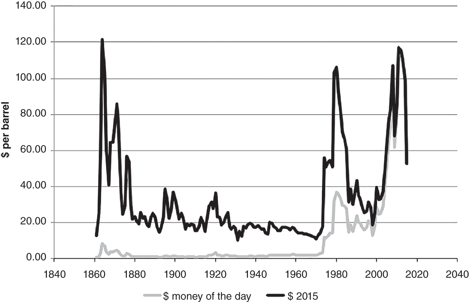
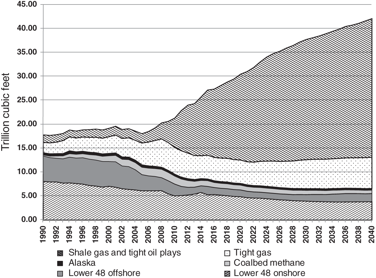
7.1.2 Unconventional Oil
7.1.3 Gas Storage
7.2 Unconventional Gas
7.2.1 Tight Gas Reservoirs
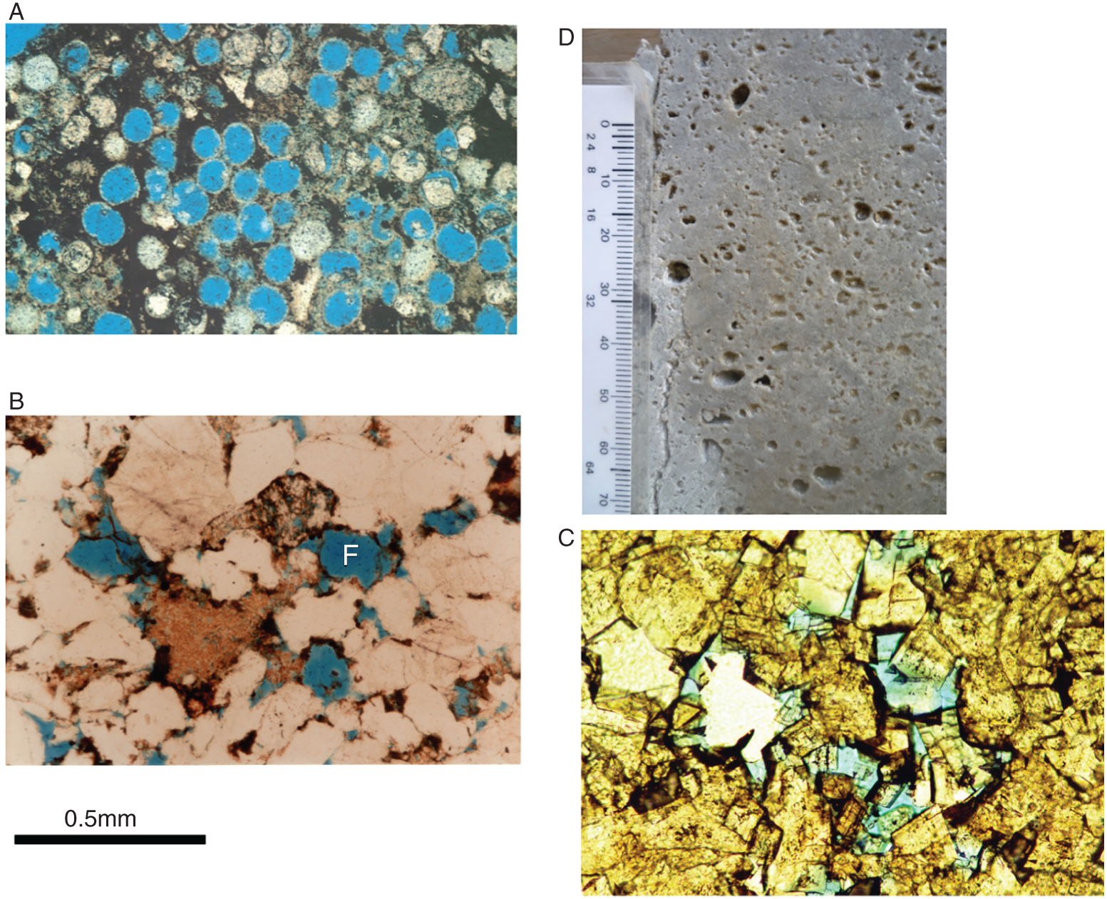
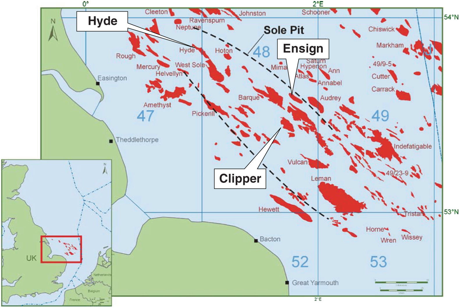
7.2.2 Shale Gas
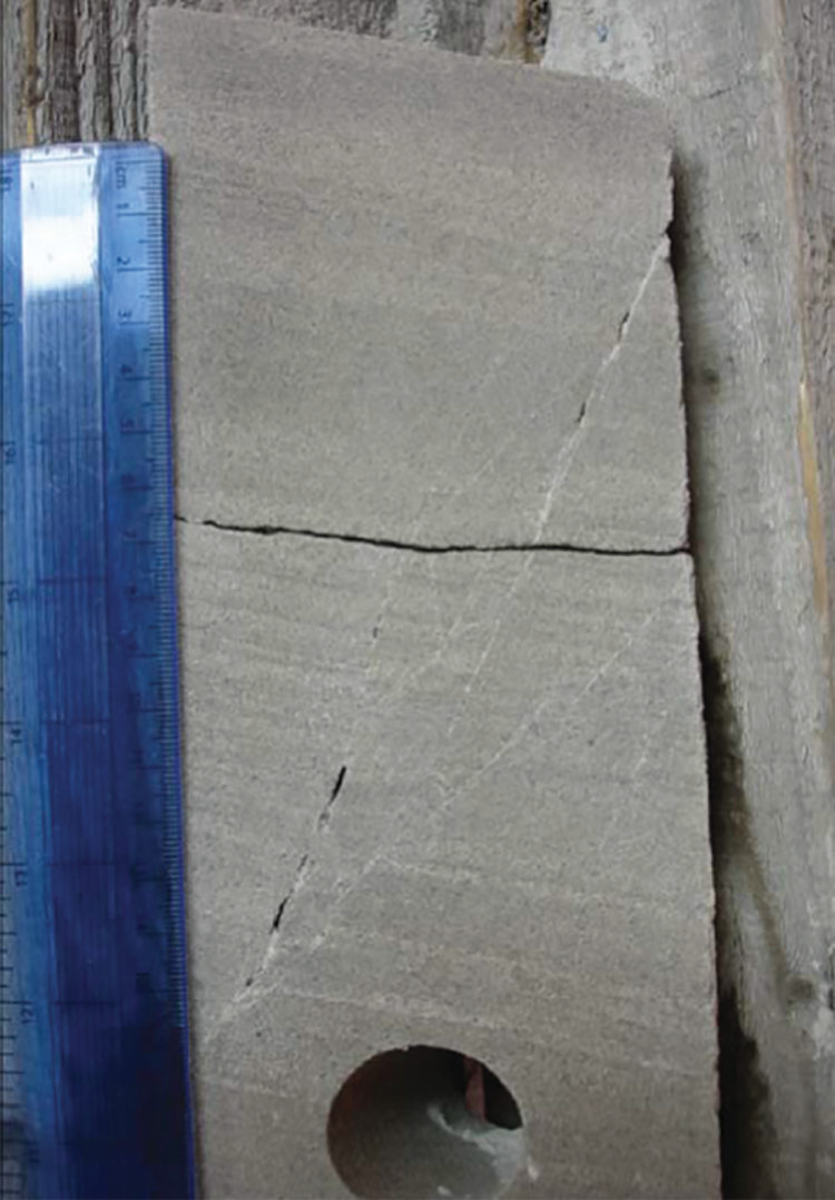
Continent
Shale resource (TCF)
North America
7.140
South America
4.569
Europe
2.587
Africa
3.962
Asia
5.661
Australasia
1.381
Total
25.300
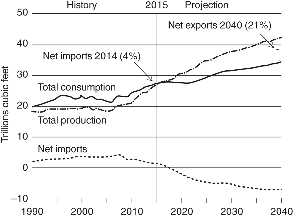
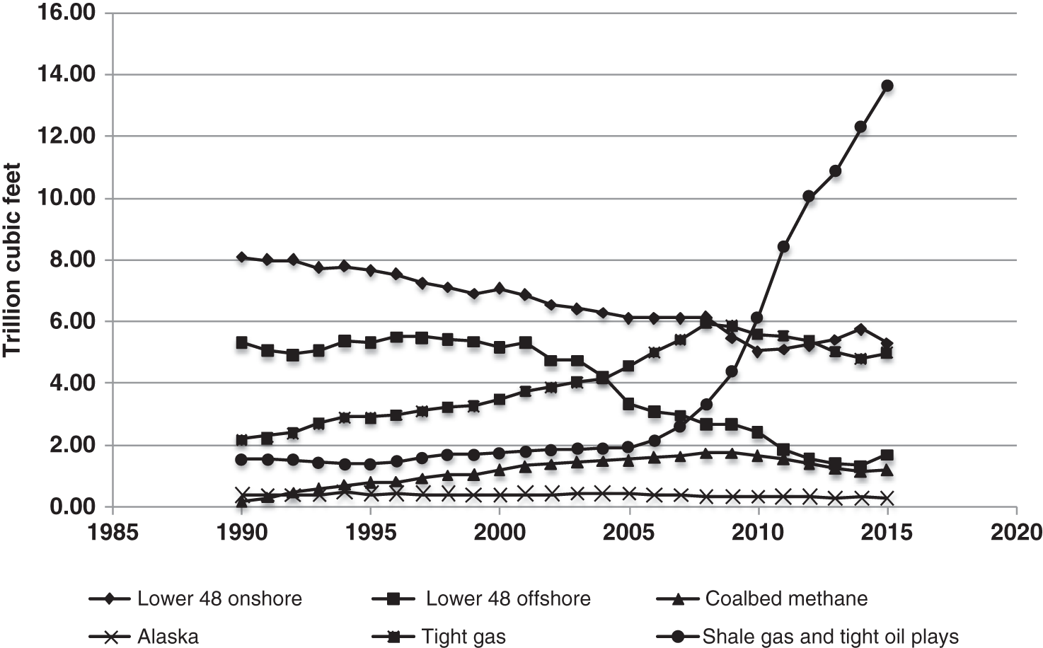
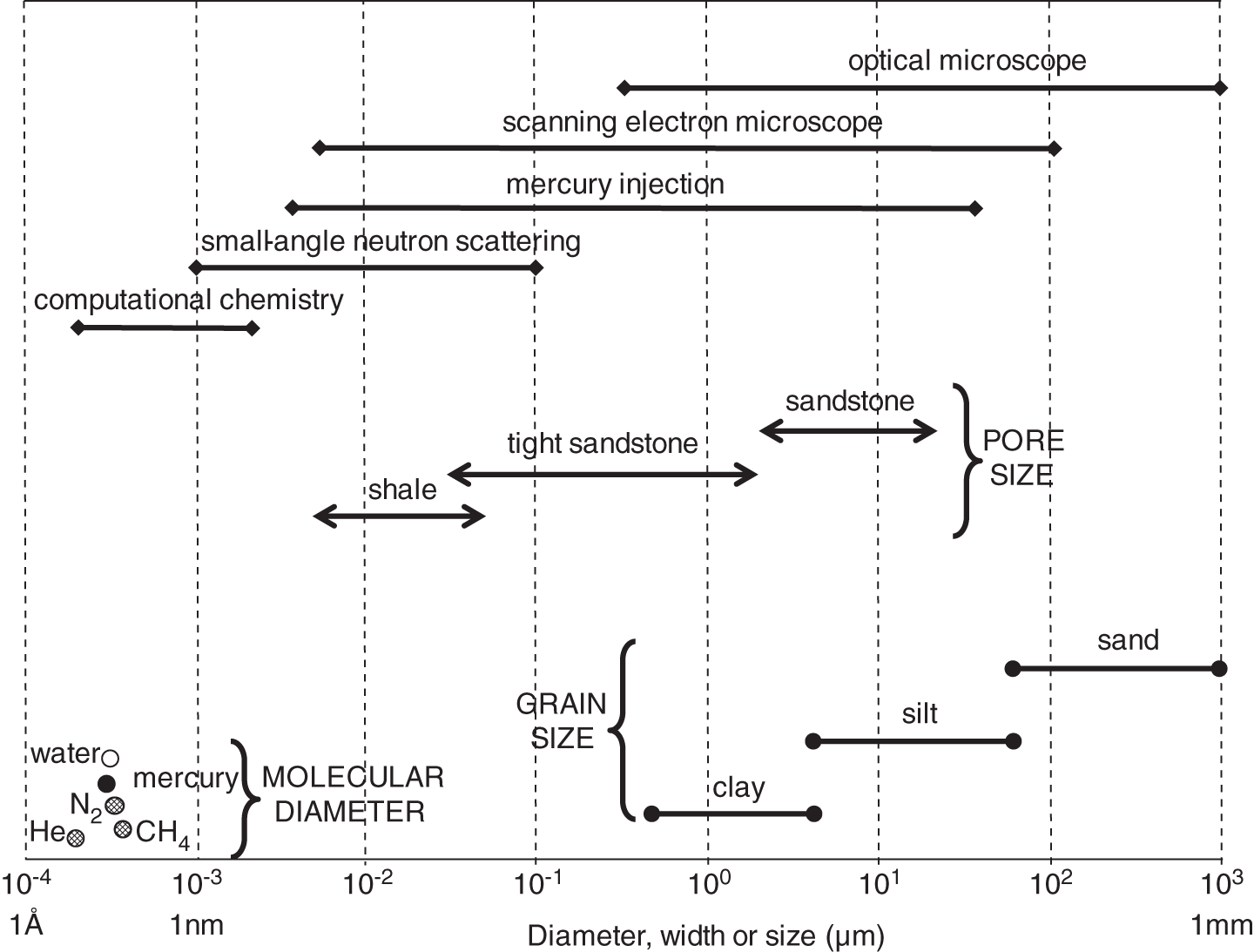
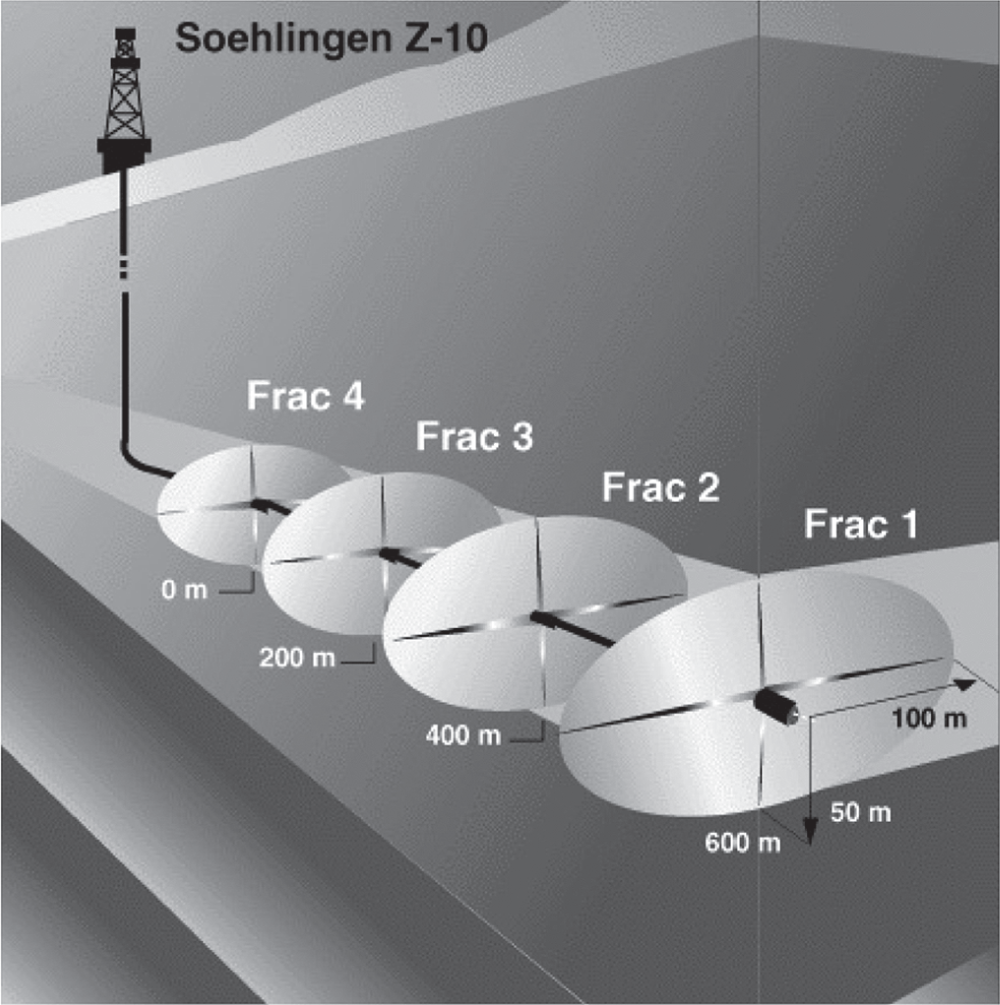
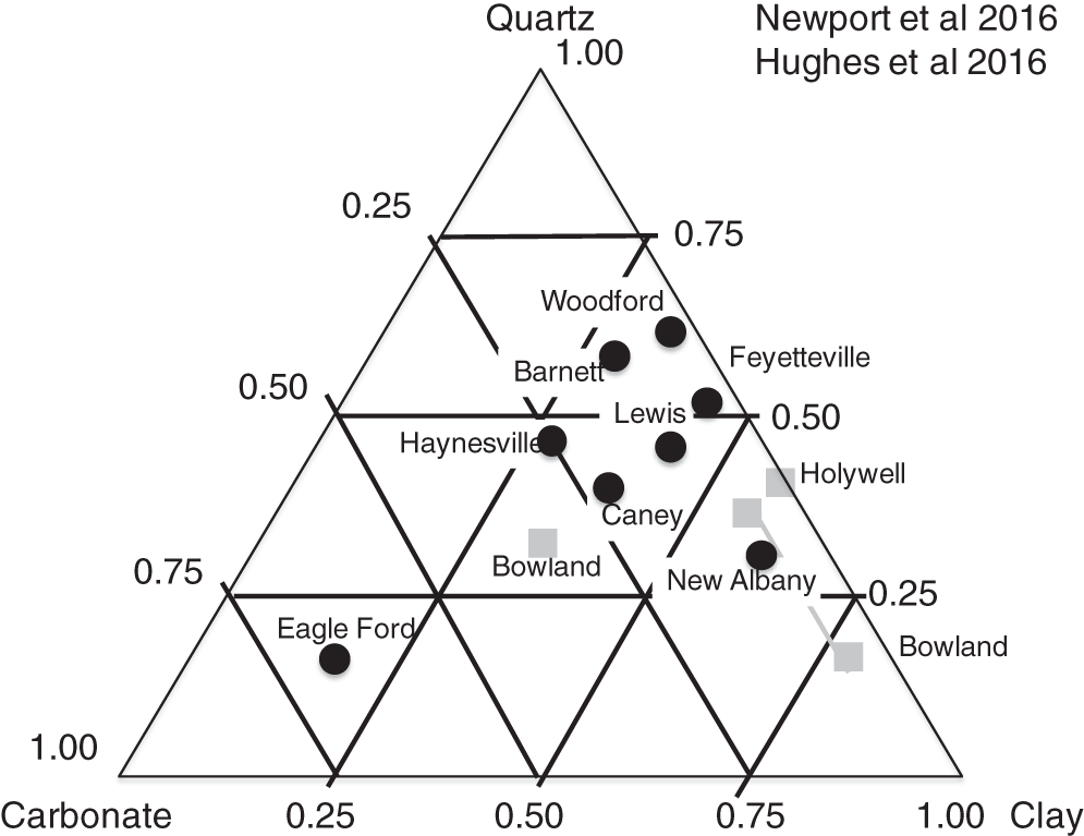
7.2.3 Low Saturation Gas
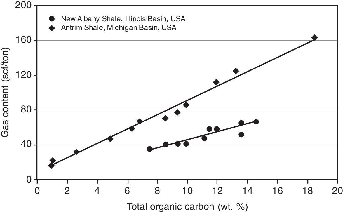
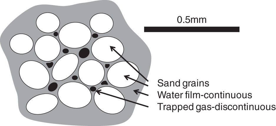
7.2.4 Shallow Gas
7.2.5 Basin-Center Gas
7.2.6 Gas Hydrates
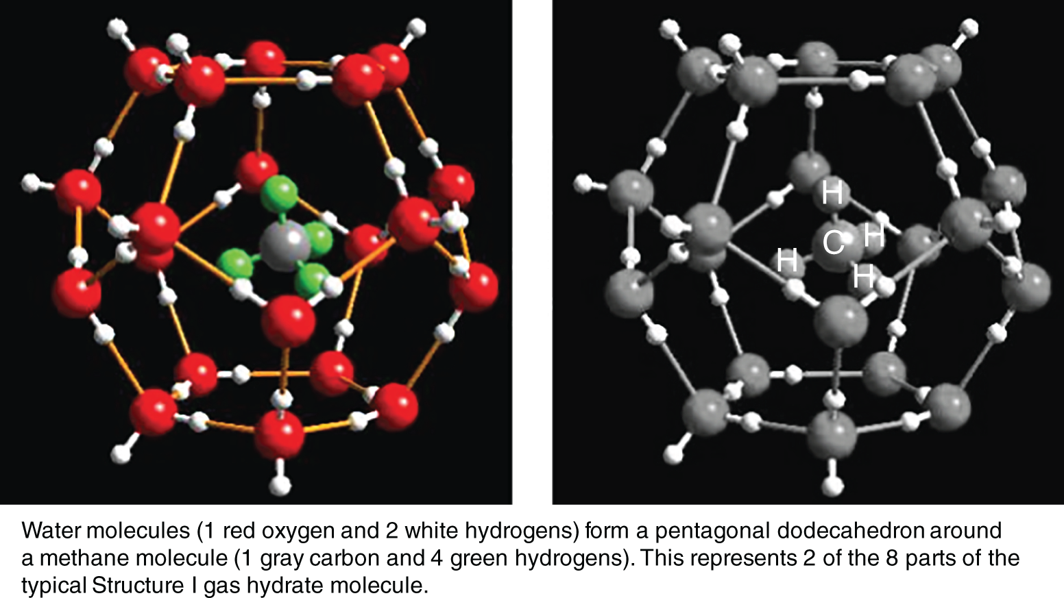
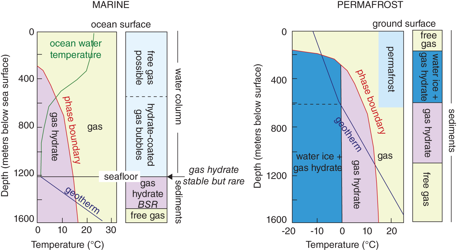
7.2.7 Coal Bed Methane
7.2.8 Coal Mine Methane
7.3 Unconventional Oil
7.3.1 Heavy Oil and Tar Sand
7.3.2 Shale Oil and Oil Shale
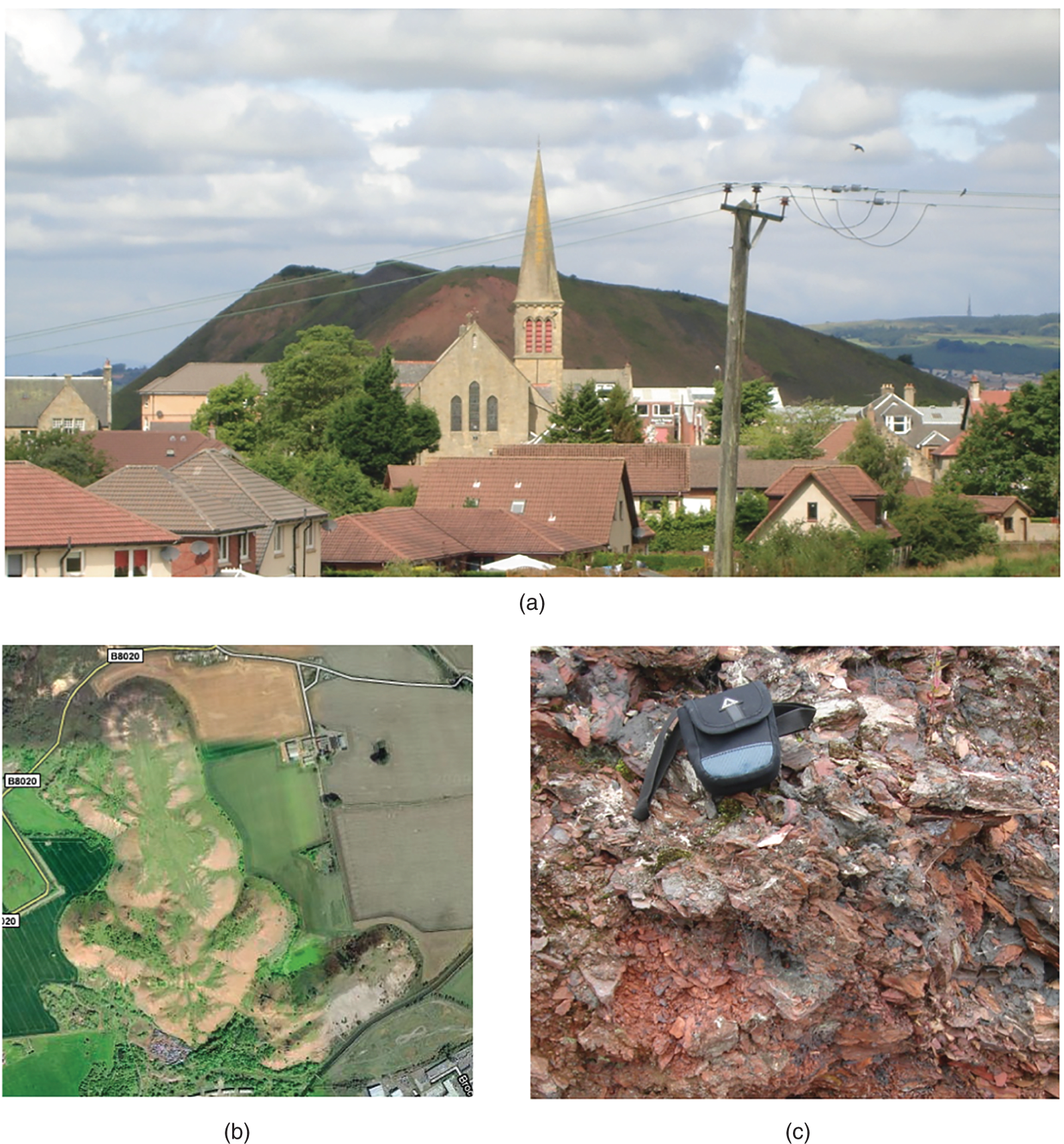
7.4 Underground Coal Gasification
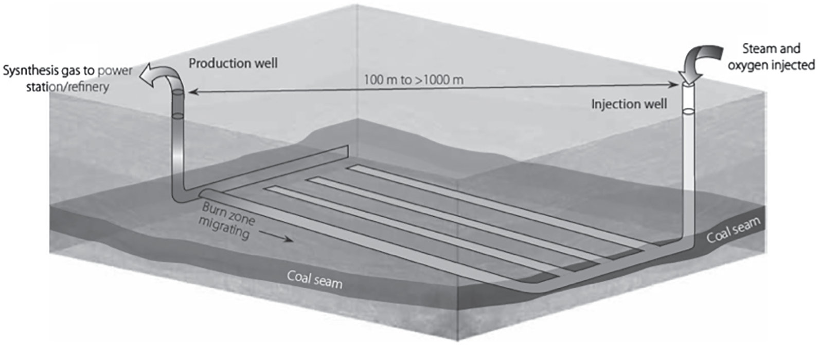
Process
Product/Use
Direct Liquefaction
Oil – fuel, chemical production
Indirect Liquefaction
Oil – fuel, chemical production
Olefin Hydroformylation
Aldehydes – plasticisers, detergents, speciality chemicals
Olefin Hydrogenation
Alkanes – fuels
Methanol Carbonylation
Acetic Acid – chemical intermediary
Hydrogen capture
Fuel, fuel Cells
7.5 Gas Storage
7.6 Carbon Storage
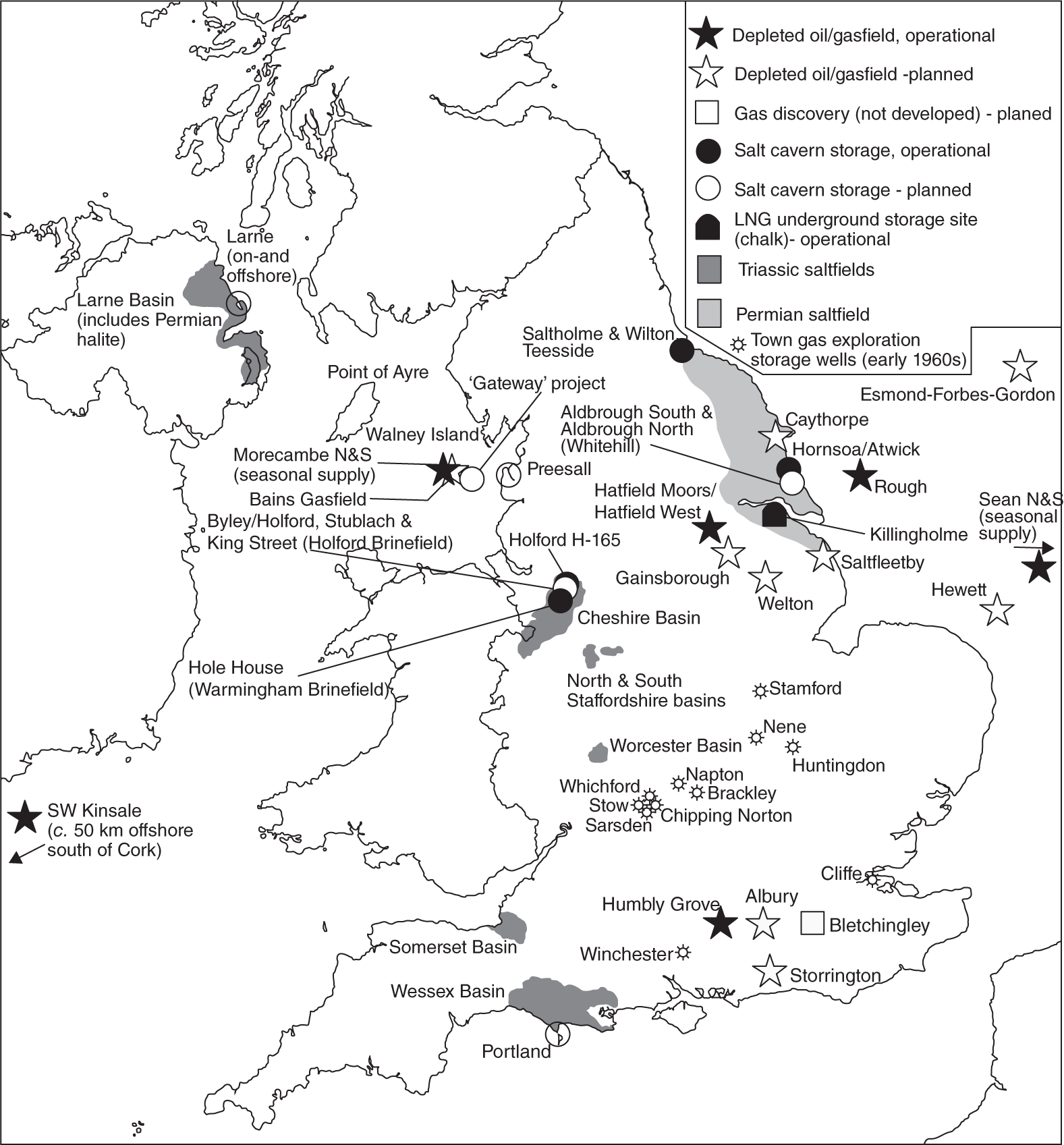
7.7 Heat, Helium, and Other Secondary Products
7.7.1 Heat Recovery
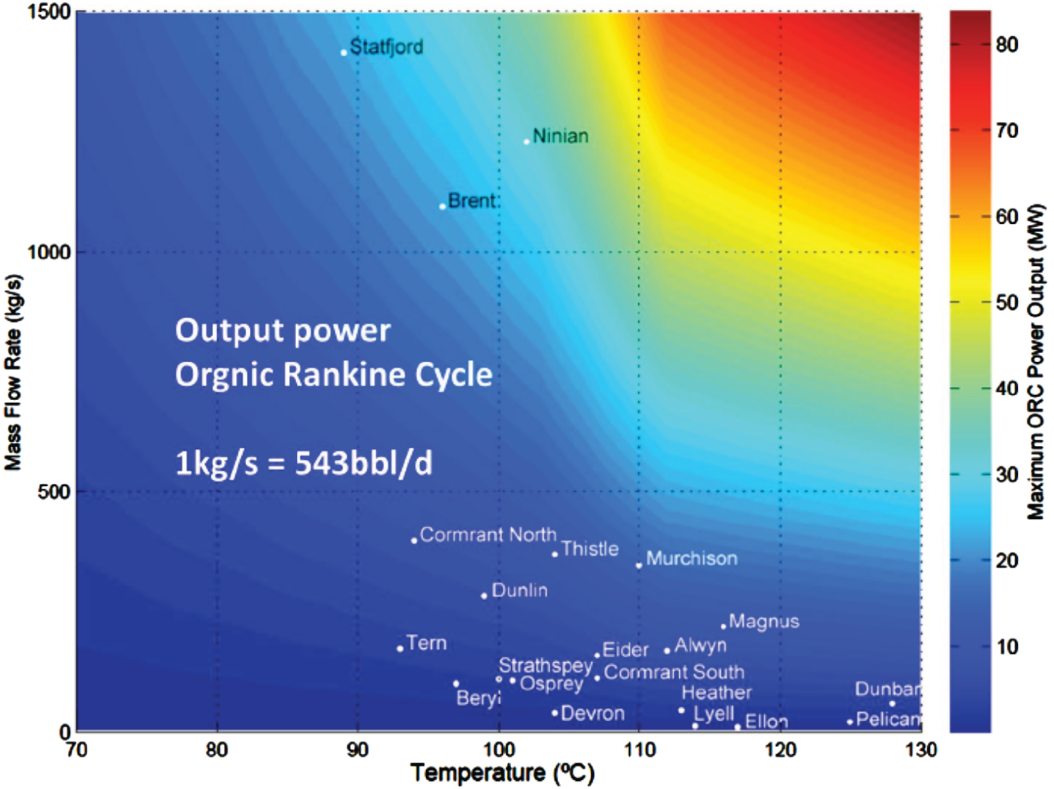
7.7.2 Lithium and Other Solutes
7.7.3 Helium
Case Histories
7.8 Dunlin Field, UK North Sea, Opportunities for Power Generation from Unconventional Gas and/or Co-Produced Water
7.8.1 Introduction
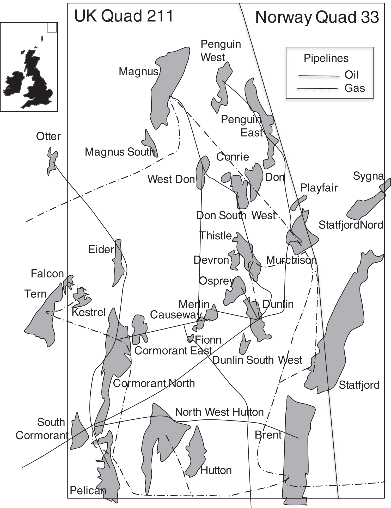
7.8.2 Deep (Shale) Gas
7.8.3 Shallow Gas
Well
Opera-tor
Interval
Depth
Notes
211/18a-17A
BNOC
U Jurassic Kimmeridgian
10 492–10 606 ft
Weak solvent crush fluorescence in claystone
2/5-10
Unocal
U Jurassic Kimmeridgian
8210–8330 ft
8550 ppm C1 plus oil
211/28-8
Shell
U Jurassic Kimmeridgian
Shows and good cut in U Jurassic sandstone (cored)
211/29-9
Shell
U Jurassic Kimmeridgian
Kimmeridge Clay Formation, light yellow fluorescence and cut, oil bleeds from core
7.8.4 Co-Produced Hot Water
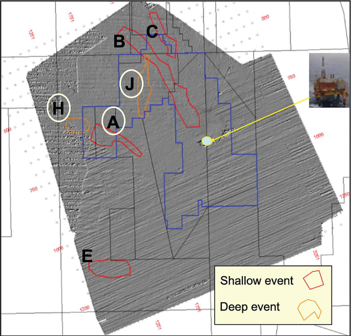
Event
A
B
C
E
H
J
Depth (two way time, secs)
0.296
0.308
0.388
0.368
0.708
0.74
Area (km2)
2.525
2.516
2.619
2.398
0.922
5.495
Thickness (m)
12
10.6
9.6
10.8
24
24
Net to gross (%)
70
70
70
70
70
70
Porosity (%)
35
35
35
35
35
35
Gas saturation (%)
70
70
70
70
70
70
Gas expansion factor
30
30
40
37
79
81
Gas in place (BCF)
5.5
4.8
6.0
5.6
9.0
55.0
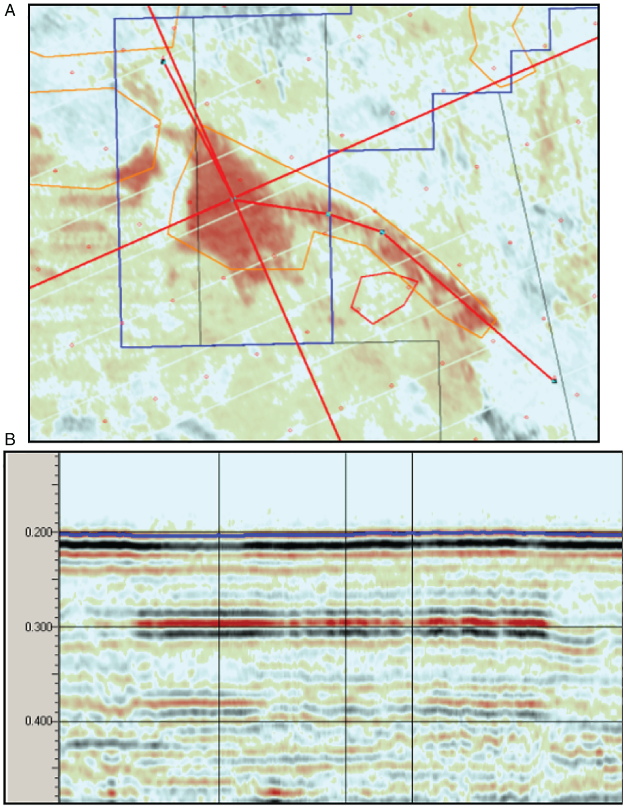
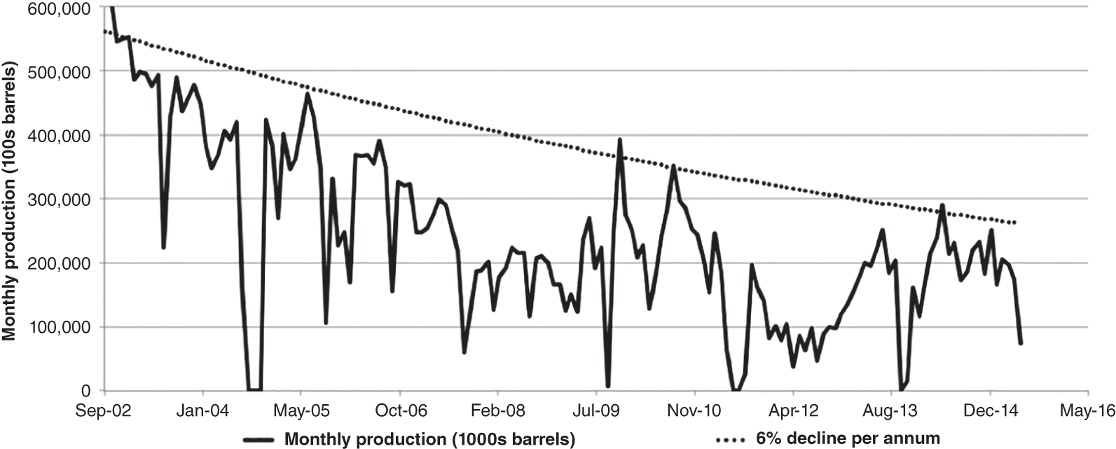
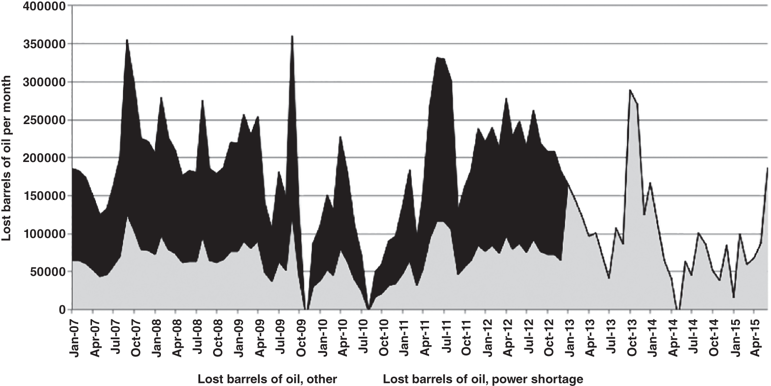
Year
Barrels oil lost production due to power outage
Average annual oil price ($)
Lost revenue ($ millions)
2007
1 563 129
64.20
100
2008
1 625 185
91.48
149
2009
1 345 597
53.48
72
2010
829 110
71.21
59
2011
1 625 805
86.46
141
2012
1 760 775
86.46
152
Total
674
7.9 Clipper South Field, UK North Sea – Development of a Tight Gas Field
7.9.1 Introduction
7.9.2 Re-Evaluation of the Field
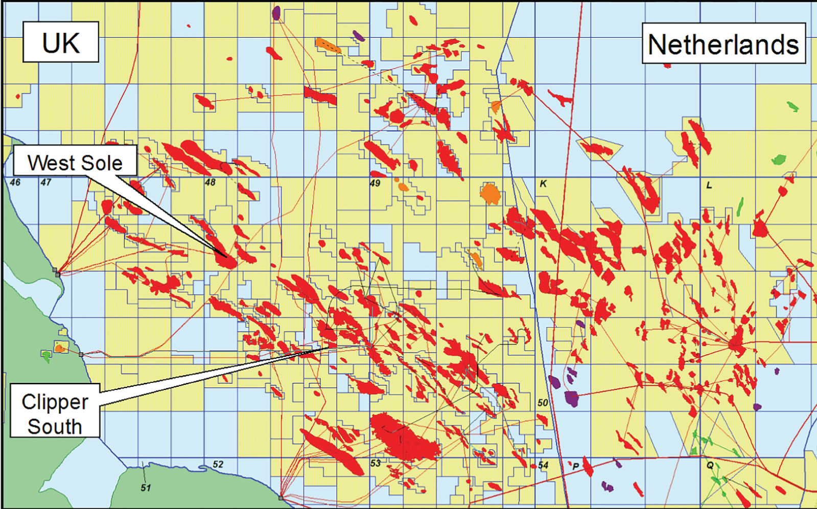
7.9.3 Analysis of Well Test Data