2.0 Introduction
The physics-based modeling of various internal flow systems in gas turbines requires a strong foundation in thermodynamics, fluid mechanics, and heat transfer. In this chapter, we review and reinforce a number of key concepts such as enthalpy, rothalpy, entropy, secondary flows, vortex, vorticity, circulation, isentropic efficiency, polytropic efficiency, stream thrust, impulse pressure, adiabatic wall temperature, and so on. Many of these concepts are directly related to the flow or fluid properties that cannot be directly measured by an instrument but are mathematical combinations of different fundamental properties. For example, the specific enthalpy is a combination of the specific internal energy and specific flow work, which is a product of static pressure and specific volume (reciprocal of density). Nevertheless, most of these derived variables play a useful role in modeling of internal flow systems and their physical interpretation. We also present here in most simple terms various laws that govern the flow and heat transfer physics. Central to any thermofluids mathematical modeling is a clear understanding of the control volume analysis of the conservation laws of mass (continuity equation), momentum (linear and angular), energy, and entropy. While large control volume analyses (macro-analyses) are at the heart of one-dimensional modeling of flow networks, small control volume analyses (micro-analyses) are invariably used in detailed predictions by computational fluid dynamics (CFD).
At the end of this chapter we have included a number of worked-out examples, which are designed to further aid in the understanding and application of various concepts and physical laws, a number of problems to help readers gauge their mastery of various topics, and references and bibliography for more detailed discussion of these topics.
2.1 Thermodynamics
The laws of thermodynamics – only the first and second laws are discussed here – are entirely based on the empirical evidence from the physical world. Accordingly, any prediction method that violates any of these laws is unlikely to yield results that are physically realizable. Thermodynamic laws involve state variables such as static pressure, static temperature, and so on, which are fluid properties, and path variables such as work transfer and heat transfer, which are needed to change the fluid properties between any two states. In our discussion in this book, we will assume that the fluid is a simple substance whose state is uniquely defined by any two properties. Additionally, the fluid is assumed to be calorically perfect with constant specific heats cpcp and cvcv, at constant pressure and constant volume, respectively. Note that these thermophysical properties are generally functions of static temperature. Consistent with our assumption, we can use an average static temperature between two consecutive states to evaluate these properties.
2.1.1 The First Law of Thermodynamics
For a closed system, the first law of thermodynamics simply states that the change in its total energy dEdE going from state 1 to state 2 results from heat transfer δQδQ and work transfer δWδW, the former is considered positive if it occurs into the system from the surroundings and the later is considered positive when the system does work on the surroundings. In equation form we can write
 (2.1)
(2.1)where the total stored energy consists of the internal energy UU, kinetic energy KEKE = mV2/2mV2/2, and potential energy PEPE (in the gravitational force field: PE = mghPE=mgh), that is,
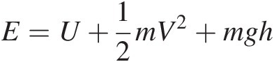 (2.2)
(2.2)For a system doing work on the surrounding, ΔV is positive. Dividing Equation 2.2 by mass mm yields
 (2.3)
(2.3)where the specific total energy e=u+12V2+gh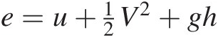 , uu being the specific internal energy. Neglecting changes in the kinetic and potential energy, Equation 2.3 becomes
 (2.4)
(2.4)When the gas volume does not change during its state change (isochoric process), Equation 2.4 reduces to du = δqdu=δq, indicating that any change in internal energy in this process is entirely as a result of heat transfer. For a calorically perfect gas, which has constant cv , we can write u = cvTsu=cvTs where we have assumed that u = 0u=0 at the reference static temperature Ts = 0Ts=0.
2.1.1.1 Enthalpy
As discussed in Section 2.2.5.4, in a flow system, the fluid specific internal energy uu appears with the quantity Ps/ρPs/ρ, which equals specific flow work as a result of pressure force. By combining these two terms, we define the static enthalpy as
 (2.5)
(2.5)Note that the static enthalpy hshs given by Equation 2.5 is a state property, which is a combination of three state properties u, Ps,u,Ps, and ρρ. Only for a flow system, Ps/ρPs/ρ can be interpreted to equal the specific flow work. For a calorically perfect gas, which has constant cpcp, we can write hs = cpTshs=cpTs where we have assumed that hs = 0hs=0 at the reference temperature Ts = 0Ts=0.
For a perfect gas with Ps = ρRTsPs=ρRTs as its equation of state, we can rewrite Equation 2.5 as
giving
as a simple relation between the two specific heats and gas constant RR.
When we add the specific kinetic energy associated with the bulk gas flow to the static enthalpy of the gas, we obtain the total specific enthalpy of the flow as
 (2.7)
(2.7)For a calorically perfect gas, we can rewrite Equation 2.7 as
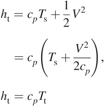 (2.8)
(2.8)which yields a simple relation between total (stagnation) temperature and total (stagnation) enthalpy.
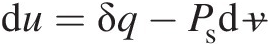
For a flow system, it is desirable to express the first law of thermodynamics in terms of enthalpy. Accordingly, we express Equation 2.4 as follows:
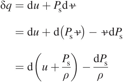
where we have used v=1/ρ . Thus, we finally obtain
 (2.9)
(2.9)For an isobaric (constant pressure) process Equation 2.9 reduces to
which shows that, for a system at constant pressure, the amount of heat transfer appears as a change in fluid static enthalpy.
2.1.2 The Second Law of Thermodynamics
The first law of thermodynamics embodies the energy conservation principle in that the energy is neither created nor destroyed; it may only be converted from one form to another. Empirical evidence shows that, while all of the work energy can be completely converted into heat energy (internal energy), the reverse is not true. The practical restriction placed on an energy conversion process is governed by the second law of thermodynamics with its focus on irreversibility, which entails conversion of organized motion to random molecular motion through the dissipation of mean flow energy by viscosity. As a result of the presence of friction in practical applications, a reversible work transfer is merely an idealization.
One of the tenets of the second law of thermodynamics is that heat transfer always occurs from higher temperature to lower temperature. This fact, for example, is built into the Fourier’s law of heat conduction governed by the equation q̇x=−kdT/dx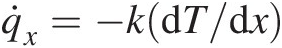 , where the negative sign ensures that the one-dimensional heat conduction in the xx direction takes place in the direction of negative temperature gradient.
2.1.2.1 Entropy
We can have an infinite number of paths connecting states 1 and 2 of a fluid system, each path with different values of heat transfer and work transfer, and the associated process could be either reversible or irreversible. According to the second law of thermodynamics, for any two reversible paths AA and BB connecting states 1 and 2, the following equality holds:
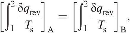 (2.11)
which points to the existence of a state property, which we call entropy. Thus, we can write
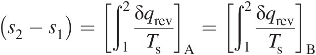 (2.12)
which is true for any reversible process connecting states 1 and 2. The second law of thermodynamics further states that the following inequality must be true for an irreversible path, say CC, connecting states 1 and 2
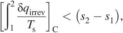 (2.13)
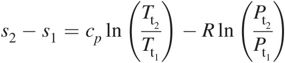
which means that a part of the entropy increase along path CC occurs as a result of irreversible work transfer. Because entropy is a state property, both reversible and irreversible processes connecting states 1 and 2 will have the same change in entropy, that is, (s2 − s1)A = (s2 − s1)B = (s2 − s1)Cs2−s1A=s2−s1B=s2−s1C. This fact gives us a means to compute entropy change between any two states. A reversible process that is also adiabatic must, therefore, be isentropic. Thus, the second law of thermodynamics provides us with an important concept of the state property called entropy, which serves to delineate the feasible flow solutions from those that are not physically possible even if they satisfy the remaining conservation equations.
Computing entropy change between two states. Let us consider a reversible process connecting two states of a fluid flow. In this case Equation 2.9 yields
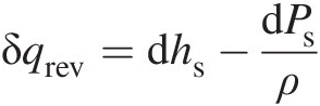
Replacing the reversible heat transfer δqrevδqrev in terms of entropy in the aforementioned equation by using Equation 2.12, we obtain
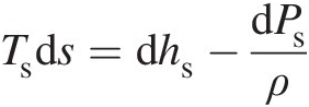 (2.14)
Because Equation 2.14 involves only state properties, it holds good for both reversible and irreversible processes connecting any two states. For a calorically perfect gas, we can write Equation 2.14 as
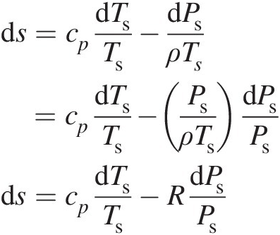 (2.15)
Integrating Equation 2.15 between states 1 and 2 yields
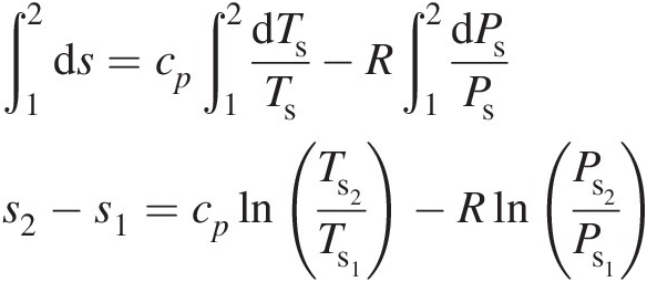 (2.16)
For an isentropic (adiabatic and reversible) process, Equation 2.16 yields
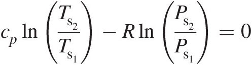 (2.17)
giving
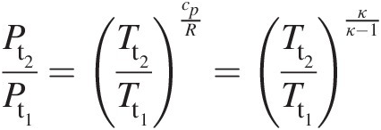
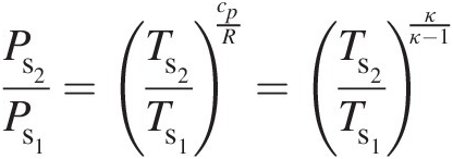 (2.18)
where κ = cp/cvκ=cp/cv. At any point in a gas flow, the total pressure and total temperature are obtained assuming an isentropic stagnation process. Accordingly, at state 1, Equation 2.18 yields
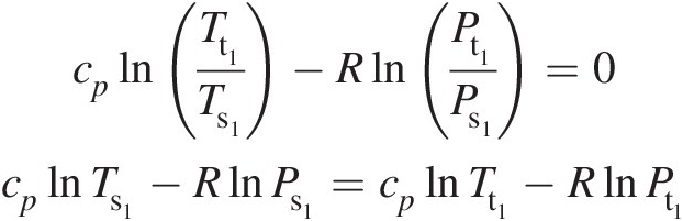 (2.19)
Similarly, we can write at state 2
Combining Equations 2.19 and 2.20, we obtain
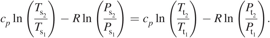 (2.21)
Thus, in terms of total pressure and total temperature, Equation 2.16 becomes
 (2.22)
Note that when we replace all static quantities in Equation 2.16 with the corresponding total quantities, we obtain Equation 2.22. For an isentropic process, Equation 2.22 yields
 (2.23)
If the total temperature in a process connecting states 1 and 2 remains constant; for example, in an adiabatic flow in a stationary duct with wall friction, Equation 2.22 reduces to
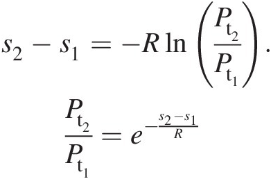 (2.24)
Because the wall friction will always increase entropy downstream of an adiabatic pipe flow, Equation 2.24 implies that the total pressure must decrease along this flow.
2.1.3 Thermodynamic Cycles
Figure 2.1a depicts the operation of a simple gas turbine on an open cycle in which both the compressor and turbine are mounted on the same shaft. In this cycle, the ambient air enters the compressor, which increases both air pressure and temperature from the specific work transfer wCwC. The compressed air temperature is further increased in the combustor through fuel addition. Hot gases (products of combustion), treated here to have properties same as air (assumed to be a perfect gas), enters the turbine, which converts part of the energy of these gases into the specific work output wTwT.
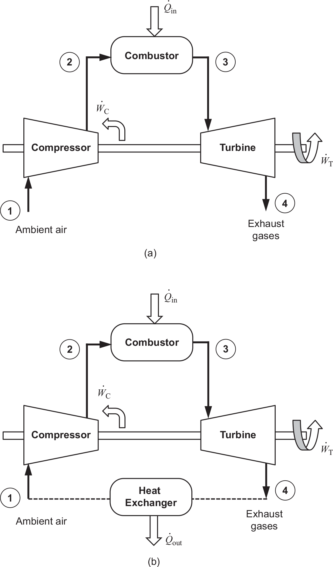
Figure 2.1 Key operational components of a simple gas turbine: (a) open cycle and (b) closed cycle with a fictitious heat exchanger.
Figure 2.1b uses a fictitious heat exchanger to cool the hot exhaust gases back to the ambient air conditions, making the gas turbine operation a closed cycle, at least thermally. From the steady flow energy equation (derived from the first law of thermodynamics) in this closed cycle we can write
 (2.25)
The thermal efficiency of an open-cycle gas turbine shown in Figure 2.1a is defined as the ratio of the net power output to the heat rate (rate of energy transfer from the combustion of fuel in the combustor), giving
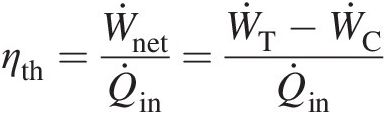 (2.26)
which also equals the cycle efficiency ηcycleηcycle for the closed-cycle gas turbine shown in Figure 2.1b.
2.1.4 Isentropic Efficiency
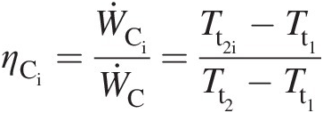
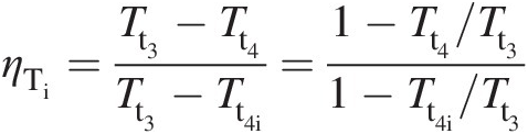
The Brayton cycle of Figure 2.2 maps the operation of the gas turbine engine shown in Figure 2.1 on the T − ST−S diagram. In this cycle, an ideal compressor operates along the isentropic process 1–2i, while the real compressor works along 1–2 with increase in flow entropy as a result of unavoidable friction and other irreversible effects present in the compressor. For the same pressure ratio πC = Pt2/Pt1πC=Pt2/Pt1, the actual compressor work input along 1–2 will be higher than the corresponding isentropic (ideal) work input along 1–2i. Accordingly, we define the compressor isentropic efficiency as follows:
 (2.27)
which further yields
 (2.28)
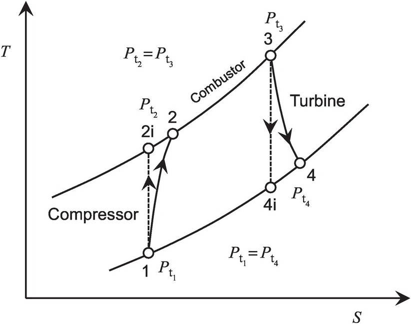
Figure 2.2 Brayton cycle of a gas turbine on T − ST−S diagram.
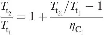
Using Equation 2.23 in Equation 2.28 results in
 (2.29)
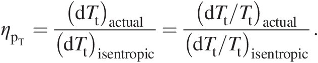
With no drop in total pressure in the combustor (Pt2 = Pt3Pt2=Pt3), the turbine inlet point 3 lies on the constant-pressure line established by the compressor exit pressure. Let us assume that the expansion in the turbine during work extraction either along the isentropic line 3–4i or the actual line 3–4 with higher entropy occurs to the same total pressure Pt4Pt4, which is equal to the compressor inlet pressure Pt1Pt1. Because point 4 lies to the right of 4i, the actual work output of the turbine along the process line 3–4 is lower than that along the isentropic (ideal) process line 3–4i. Accordingly, we define the turbine isentropic efficiency as follows:
 (2.30)
which further yields
 (2.31)
Substitution of Equation 2.23 in Equation 2.31 gives
 (2.32)
where πT = Pt3/Pt4πT=Pt3/Pt4 is the pressure ratio across the turbine and equals the pressure ratio πC = Pt2/Pt1πC=Pt2/Pt1 across the compressor.
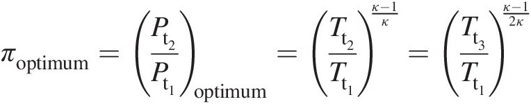
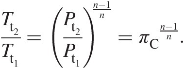
With reference to the gas turbine cycle shown in Figure 2.2, we can express the cycle efficiency or the thermal efficiency in terms of total temperatures as follows:
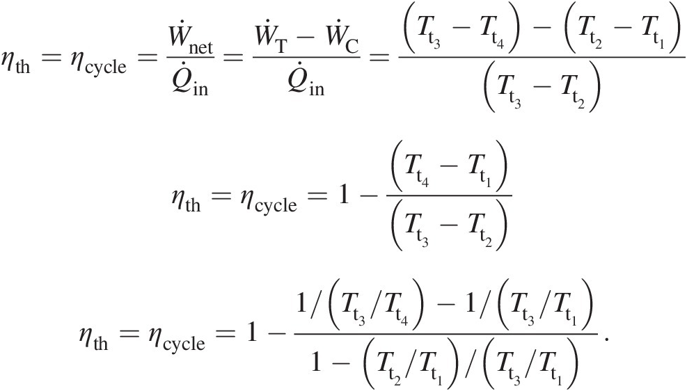 (2.33)
In Equation 2.33, the temperature ratio Tt2/Tt1Tt2/Tt1 across the compressor is given by Equation 2.28 and the temperature ratio Tt3/Tt4Tt3/Tt4 across the turbine by Equation 2.32. The equation involves an additional parameter Tt3/Tt1Tt3/Tt1, which is the ratio of turbine inlet temperature to compressor inlet temperature. For an ideal Brayton cycle with ηCi = ηTi = 1.0ηCi=ηTi=1.0, which for πC = πTπC=πT implies that Tt2/Tt1 = Tt3/Tt4Tt2/Tt1=Tt3/Tt4, Equation 2.33 simplifies to
 (2.34)
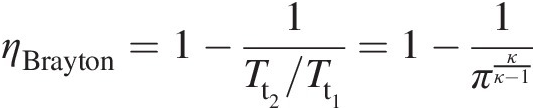
where π = πC = πTπ=πC=πT. It is interestingly to note from Equation 2.34 that ηBraytonηBrayton is independent of the parameter Tt3/Tt1Tt3/Tt1.
Both Equations 2.33 and 2.34 are plotted in Figure 2.3, showing variation of gas turbine cycle efficiency with pressure ratio π = πC = πTπ=πC=πT. The ideal Brayton cycle efficiency ηBraytonηBrayton with ηCi = ηTi = 1.0ηCi=ηTi=1.0 shown in the figure increases monotonically with pressure ratio, initially rather sharply for π < 10π<10 and then gradually reaching a value of 0.673 for π = 50π=50. The trend of cycle efficiency variation with pressure ratio with nonideal compressor and turbine depends upon the ratio of turbine inlet temperature to compressor inlet temperature as shown in the figure for ηCi = ηTi = 0.9ηCi=ηTi=0.9. For Tt3/Tt1 = 4Tt3/Tt1=4, cycle efficiency first increases with pressure ratio, reaches a maximum value of 0.380 at π = 18π=18, and then decreases to ηcycle = 0.191ηcycle=0.191 at π = 50π=50. The curve for Tt3/Tt1 = 5Tt3/Tt1=5 exhibits a shallower maximum that corresponds to ηcycle = 0.447ηcycle=0.447 at π = 33π=33, decreasing to ηcycle = 0.433ηcycle=0.433 at π = 50π=50. The figure also shows a well known result that, for a given pressure ratio and compressor inlet temperature, the cycle efficiency increases with turbine inlet temperature.
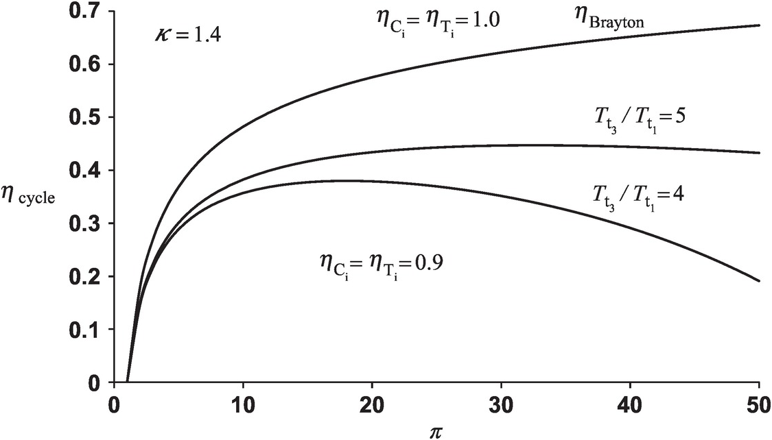
Figure 2.3 Variation of gas turbine cycle efficiency with pressure ratio.
Optimum pressure ratio for maximum net specific work output. With reference to Figure 2.2, we can express the net specific work output (turbine specific work output minus compressor specific work input, neglecting the fuel mass addition in the combustor) as
Because Tt2/Tt1 = Tt3/Tt4Tt2/Tt1=Tt3/Tt4, we obtain Tt4/Tt1 = Tt3/Tt2Tt4/Tt1=Tt3/Tt2. We now rewrite Equation 2.35 as
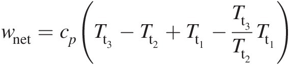
which for an optimum value of wnetwnet with respect to Tt2Tt2 yields
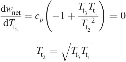 (2.36)
Equation 2.36 further leads to
 (2.37)
which, for a given ratio of turbine inlet temperature to compressor inlet temperature, yields the optimum pressure ratio across the compressor needed for maximum net specific work output of the gas turbine. Note that, in the aforementioned derivation, we have assumed a single value of κκ, which is typically close to 1.4 for the compressor and 1.33 for the turbine.
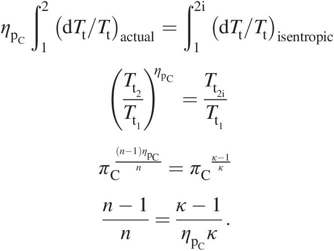
2.1.5 Polytropic Efficiency
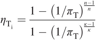
In a gas turbine, the isentropic efficiencies of compressor and turbine depend upon their operating conditions. For example, if two identical compressors operate in series with equal pressure ratio across each, their isentropic efficiency will be equal. This isentropic efficiency, however, will be higher than if the same compressor were to operate over the higher combined pressure ratio. This results from the fact that the increase in entropy as a result of friction in the upstream compressor requires more work input in the downstream one, generally known as the preheat effect. If we divide the compression process across a compressor or the expansion process across a turbine into a large number of very small, consecutive compression or expansion processes, respectively, then the isentropic efficiency across each is called the polytropic efficiency, or small-stage efficiency, which may be assumed constant for the machine, reflecting its state-of-the-art design engineering.
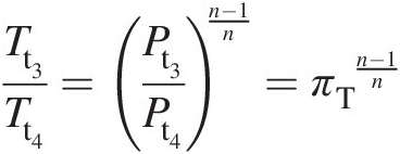
With reference to Figure 2.2, we assume that the index of polytropic compression along 1–2 is nn, which yields
 (2.37)
Note that, for n = κn=κ, this equation yields the isentropic compression along 1–2i.
We define the compressor polytropic efficiency as
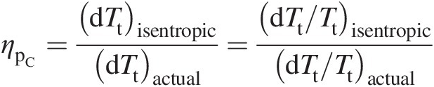 (2.38)
Integrating Equation 2.38 between the compressor inlet and exit yields
 (2.39)
To establish a relation between the compressor isentropic efficiency and its polytropic efficiency, we write
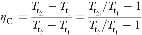
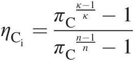
which with the substitution of Equation 2.39 yields
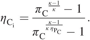 (2.40)
Equation 2.40 expresses compressor isentropic efficiency in terms of its polytropic efficiency and pressure ratio. Alternatively, to express compressor polytropic efficiency in terms of its isentropic efficiency and pressure ratio, we can rewrite Equation 2.40 as
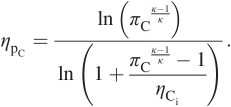 (2.41)
Again, with reference to Figure 2.2, we assume that the index of polytropic expansion in the turbine along 3–4 is nn, which yields
 (2.42)
Note that for n = κn=κ, the aforementioned equation yields the isentropic expansion along 3–4i.
We define the turbine polytropic efficiency as
 (2.43)
Integrating Equation 2.43 across the turbine yields
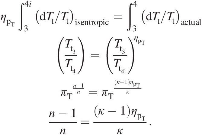 (2.44)
To establish a relation between the turbine isentropic efficiency and its polytropic efficiency, we write
which using Equation 2.44 yields
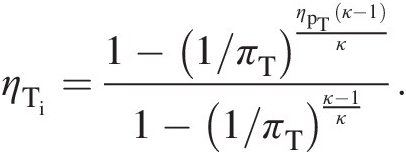 (2.45)
Equation 2.45 expresses turbine isentropic efficiency in terms its polytropic efficiency and pressure ratio. Alternatively, to express turbine polytropic efficiency in terms of its isentropic efficiency and pressure ratio, we rewrite Equation 2.45 as
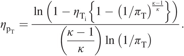 (2.46)
Equations 2.40 and 2.45 are plotted in Figure 2.4 for ηpC = ηpT = 0.9ηpC=ηpT=0.9. In this figure, we have assumed κ = 1.4κ=1.4 for the compressor and κ = 1.33κ=1.33 for the turbine. For the pressure ratio very close to 1.0, the compressor and the turbine each has equal isentropic and polytropic efficiencies. The figure further shows that, for the compressor, the isentropic efficiency decreases with pressure ratio and, for the turbine, it increases with the pressure ratio. The rate of efficiency decrease for the compressor, however, is higher than the corresponding rate of efficiency increase for the turbine.
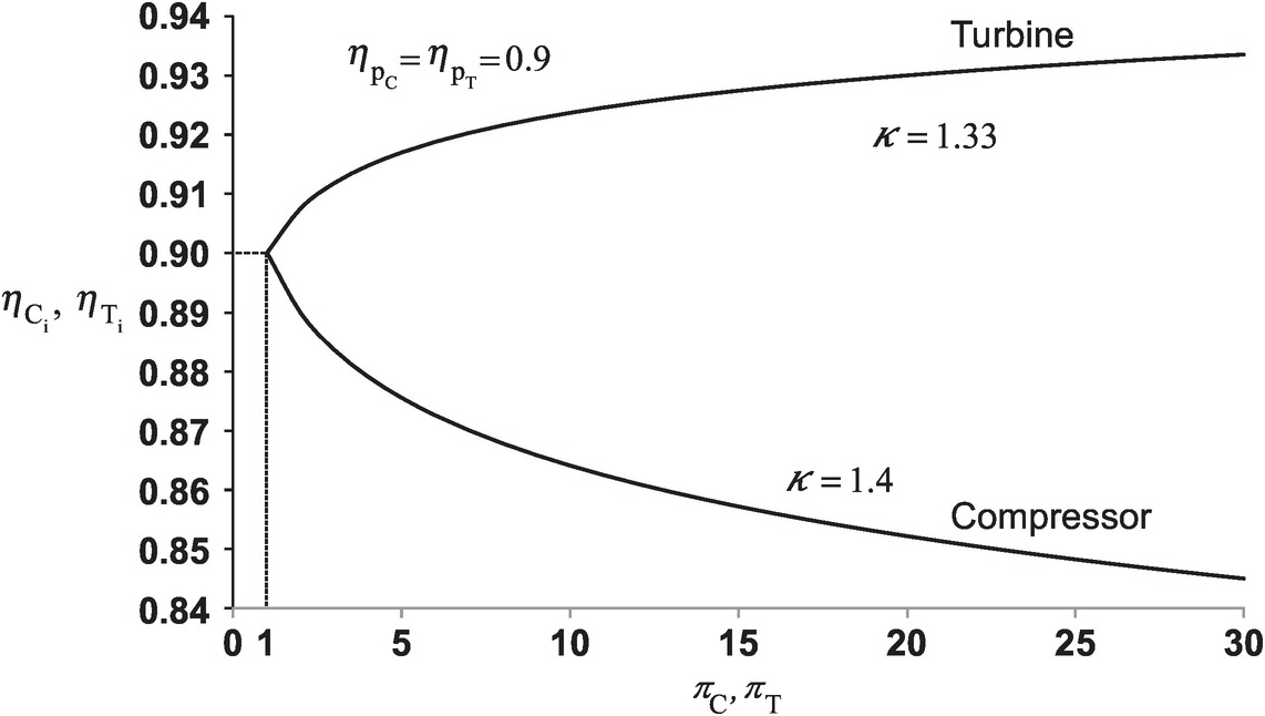
Figure 2.4 Variation of compressor and turbine isentropic efficiencies with pressure ratio for a constant value of their polytropic efficiency.
2.2 Fluid Mechanics
2.2.1 Secondary Flows
In a gas turbine operation, flows that directly partake in the energy conversion along the turbine and compressor flow path (core flow) are generally referred to as the primary flows. The flows that are used for cooling and sealing of gas turbine components are often called secondary flows. These flows should not be confused with the secondary flows, which are normal to the main flow direction, found in many internal flows. For example, a turbulent flow in a noncircular duct features secondary flows that have velocities in the plane of the duct cross-section, which is perpendicular to the main flow direction. These are driven by the anisotropy in turbulence intensity and gradients in normal turbulent stresses and are called secondary flow of the second kind. Note that these secondary flows do not exist in a constant-viscosity laminar flow in a noncircular duct or the turbulent flow in a circular duct.
Because the local gradient in static pressure is the common primary mechanism to generate the velocity field in a flow, when a uniform flow enters a bend in a circular duct it exits with secondary flows. In the bend region, as a result of the centrifugal force, the static pressure at the outer radius of curvature is higher than at the inner radius of curvature. This radial pressure gradient in the pipe cross-section generates secondary flows that we observe at the exit plane. These are known as the secondary flows of the first kind.
2.2.2 Vorticity and Vortex
Vorticity is a kinematic vector property of a flow field and equals the curl of its velocity vector (ζ→=∇×V→ ). At any point in the flow, the vorticity represents the local rigid-body rotation of fluid particles and equals twice the rotation vector (ζ→=2ω→
 ). A vortex, on the other hand, refers to the bulk circular motion of the entire flow field. Streamlines in a vortex flow are essentially concentric circles, and so are the isobars (lines of constant static pressure). The local pressure gradient along the radius of curvature is given by the local equilibrium equation dPs/dr=ρVθ2/r
 . This characteristic of a vortex flow is so different from a nonrotating flow where the static pressure typically varies along a streamline, as dictated by the Bernoulli equation for an ideal incompressible flow.
A forced vortex features bulk rigid-body rotation with constant angular velocity (in radians per second) for all streamlines. As a result, the outer streamline features higher tangential, or swirl, velocity than the inner ones. In a free vortex, which is assumed to be free from any external torque, the angular momentum (the product of radius and tangential velocity), not the angular velocity, remains constant everywhere in the flow. In this vortex, the outer streamline has lower tangential velocity than the inner one. As a result of the presence of centrifugal force, all vortex motions feature positive radial gradient in the static pressure distribution. Lugt (1995) presents an excellent discussion of vortex flows in both nature and technology.
2.2.3 Sudden Expansion Pipe Flow With and Without Swirl
In gas turbine design applications, flows often feature changes in pipe diameter, going from a smaller-diameter pipe to a larger-diameter pipe (sudden expansion) or from a larger-diameter pipe to a smaller-diameter pipe (sudden contraction). Such flows, with their undesirable excess loss in total pressure, generally become necessary as a result of spatial constraints.
Following a sudden expansion, shown in Figure 2.5a for the case without swirl, the flow enters the larger pipe in the form of a circular jet whose shear layer grows both inward toward the pipe axis and outward toward the pipe wall. While the inward growth of the shear layer occurs at the expense of the potential (inviscid) core flow, which decays downstream until the shear layers merge at the pipe axis, its outward growth happens through the process of entrainment until it finally reattaches to the pipe wall. The fluid entrained into this shear layer is continuously replenished from downstream through a favorable reverse pressure gradient. This gives rise to a primary recirculation region such that the flow in its forward branch is driven by the central jet momentum, and in its reverse branch, by an adverse pressure gradient. Sultanian, Neitzel, and Metzger (1986) present accurate CFD predictions of this flow field using an advanced algebraic stress transport model of turbulence. They also demonstrate that the standard high-Reynolds number κ − εκ−ε turbulence model significantly under-predicts the experimentally found reattachment lengths.
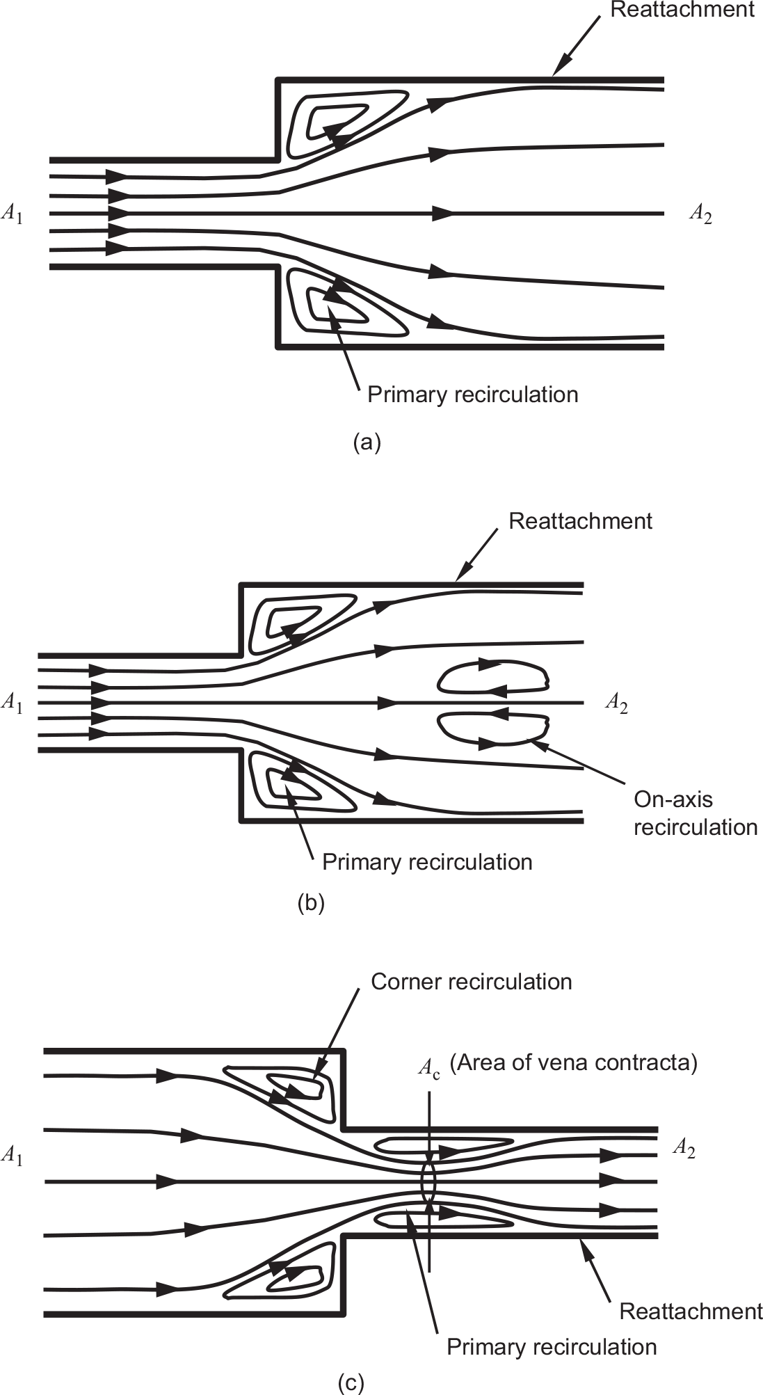
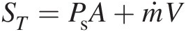
Figure 2.5 (a) Sudden expansion pipe flow without swirl, (b) Sudden expansion pipe flow with swirl, and (c) Sudden contraction pipe flow without swirl.
Figure 2.5b shows the main features of a swirling flow in a sudden pipe expansion. The wall-bounded primary recirculation zone in this flow field is found to shrink with the increasing incoming swirl velocity. When the swirl exceeds a critical value (greater than 45-degree swirl angle), an on-axis recirculation region appears. Sultanian (1984) discusses at length the overwhelming complexity of this flow field from a computational viewpoint. The major difficulties associated with predicting this three-dimensional flow field lies in accurately modeling its highly anisotropic turbulence field.
A distinguishing feature of a critically swirling flow in a sudden pipe expansion is the region of on-axis recirculation caused by vortex breakdown. Such a feature is widely used in modern gas turbine combustors as an aerodynamic flame holder, which in early designs corresponded to the wake region of a bluff body, to ignite the fresh charge entering the combustor. Here is a simple explanation behind the vortex breakdown in this flow field. The swirl in a free or forced vortex causes positive radial pressure gradient, that is, the static pressure always increases radially outward – the higher the swirl, the higher is this pressure gradient. Near the sudden expansion, as a result of high swirl, the static pressure at the pipe axis is much lower than the section-average static pressure. Further downstream, swirl decays as a result of wall shear stress, and the static pressure distribution tends to become more uniform over the pipe cross section. As a result, the static pressure at the pipe axis becomes higher downstream than upstream, causing on-axis flow reversal.
2.2.4 Sudden Contraction Pipe Flow: Vena Contracta
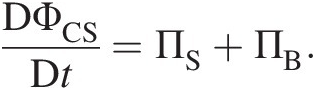
Key features of a sudden contraction pipe flow are shown in Figure 2.5c. When the flow from the large pipe of area A1A1 abruptly enters the smaller pipe of area A2 < A1A2<A1, the outer streamline detaches from the pipe wall near the area change, creating a short region of corner recirculation and the minimum flow cross-section, called the vena contracta, in the downstream pipe. At the vena contracta, having area Ac < A2Ac<A2 and surrounded by the primary recirculation zone in the downstream pipe, the flow has the maximum velocity and minimum static pressure. Downstream of the vena contracta, the flow behaves very similar to the one in a sudden pipe expansion, discussed in Section 2.2.2, expanding from AcAc to A2A2. Experimental data in a sudden contraction pipe flow indicate that Ac/A2Ac/A2 is a function of A1/A2A1/A2. For example, Ac/A2 = 0.68Ac/A2=0.68 for A1/A2 = 2A1/A2=2. It is worth noting here that, for given A1/A2A1/A2, AcAc does not depend on the total-to-static pressure ratio at the vena contracta for incompressible flows but increases slightly for compressible flows.
2.2.5 Stream Thrust and Impulse Pressure
The concept of stream thrust is grounded in the linear momentum equation. The stream thrust at any section of an internal flow, be it incompressible or compressible, is defined as the sum of the pressure force and inertia force (momentum flow rate). In any particular direction, the stream thrust thus represents the total force of the flow stream – we need this much force in the opposite direction to bring the flow velocity to zero (stagnation). For example, the force needed to hold a plate in place to an incoming fluid jet equals the stream thrust associated with the jet, and not the jet area times the jet stagnation pressure at the plate. As another example, let us consider a constant-area duct with zero wall friction, say a stream tube. The stream thrust associated with an incoming flow with nonuniform velocity distribution will remain constant throughout the duct, although its static pressure and total pressure at each section will change downstream. If the velocity profile is uniform at the duct exit, its static pressure will be higher and total pressure lower than their respective values at the duct inlet.
Given by the equation
 (2.47)
the stream thrust is a vector quantity having the same direction as the momentum velocity (see Section 2.2.5) in the chosen coordinate system. Use of stream thrust at inlets and outlets of a control volume for the momentum equation in each coordinate direction makes it analogous to the continuity and energy equations, which involve only scalar quantities. The net change in stream thrust summed over all inflows and outflows of a control volume must equal all body and surface forces (except the pressure forces at inlets and outlets) acting on the control volume.
Impulse pressure equals the stream thrust per unit area. It is given by the equation
which is valid for both incompressible and compressible flows. The aforementioned equation should not be confused with the equation Pt = Ps + ρV2/2Pt=Ps+ρV2/2, which is used to compute total pressure in an incompressible flow and approximately in a compressible flow at low Mach numbers (M ≤ 0.3M≤0.3). Note that the second term on the right-hand side of Equation 2.48 equals twice the dynamic pressure of an incompressible flow.
2.2.6 Control Volume Analyses of Conservation Laws
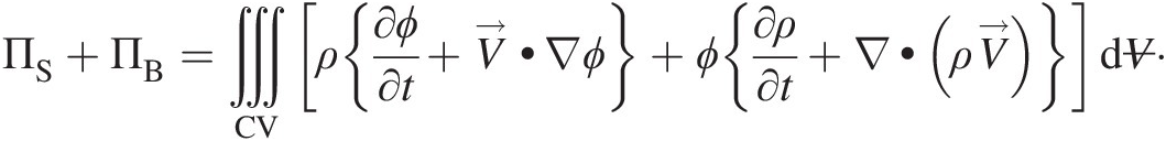
Control volume analyses of the conservation laws of mass, momentum, energy, and entropy form the core foundation for the mathematical modeling of all fluid flows and their quantitative predictions for practical applications. In Newtonian mechanics, conservation laws are written in an inertial reference frame for a control system of identified mass – the Lagrangian viewpoint. If ΦCSΦCS stands for the mass, linear momentum, energy, or entropy of a control system with the corresponding intensive (per unit mass) properties represented by ϕϕ, the substantial, total, or material derivative of ΦCSΦCS in a flow field, where the control system instantaneously assumes the local flow properties, can be written as
 (2.49)
In Equation 2.49, the terms on the right-hand side are the change agents, ΠSΠS working on the surface of the control system and ΠBΠB working on the body of the control system. Their net effect is to cause DΦCS/DtDΦCS/Dt on the left-hand side of the equation. Note that ΦCSΦCS is the instantaneous value of the extensive property ΦΦ for the entire control system.
In most engineering applications, a control volume analysis consistent with the Eulerian viewpoint is used. Facilitated by the Reynolds transport theorem, see Sultanian (2015), the left-hand side of Equation 2.49 can be replaced by
 (2.50)
in which the first term on the right-hand side represents the time rate of change of ΦΦ within the control volume and the second term represents the net outflow (total outflow minus total inflow) of ΦΦ through the control volume surface.
Combining Equations 2.49 and 2.50, we obtain
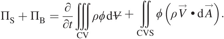 (2.51)
Invoking Gauss divergence theorem, we can replace the surface integral in Equation 2.51 by volume integral, giving
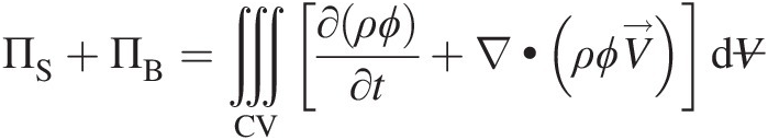 (2.52)
where we have assumed that ∂V/∂t=0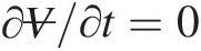 , allowing us to pull ∂/∂t∂/∂t inside the volume integral. Note that Equation 2.51 is convenient to use for an integral control volume analysis, and Equation 2.52 forms the basis for a point-wise differential control volume analysis.
2.2.6.1 Mass Conservation (Continuity Equation)
According to the law of mass conservation we must have ΠS = ΠB = 0ΠS=ΠB=0 as there can be no agent that will change the mass of a system. In this case, we have ϕ = 1ϕ=1, and Equation 2.51 reduces to
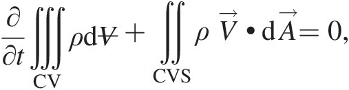 (2.53)
which simply states that, for a given control volume with multiple inlets and outlets, the imbalance between mass inflows and outflows equals the rate of accumulation or reduction of mass in the control volume.
For ϕ = 1ϕ=1, Equation 2.52 reduces to the volume integral
whose integrand must be zero, giving
 (2.54)
Note that Equation 2.54, which is a partial differential equation, must be satisfied at every point in a flow field. For a steady compressible flow, the continuity equation becomes ∇•ρV→=0 , and for an incompressible flow, be it steady or unsteady, we obtain ∇•V→=0
 , which states that the velocity field of an incompressible flow must be divergence free.
Expanding terms within the volume integral on the right-hand side of Equation 2.52, using the vector identity for the divergence term involving scalar coefficients, and regrouping them, we obtain
Using Equation 2.54, the expression within the second curly brackets in the right-hand side of the aforementioned equation becomes zero. We finally obtain a simpler form of Equation 2.52
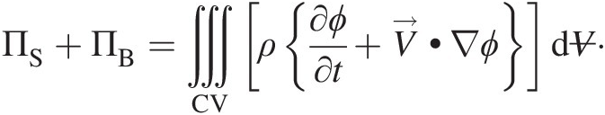 (2.55)
2.2.6.2 Linear Momentum Equation
The linear momentum equation for a system is grounded in the Newton’s second law of motion, which simply states that the force acting on a system equals the mass of the system times its acceleration in the direction of the force. So the forces acting on a system are the change agent for its linear momentum. Accordingly, Equation 2.52 for the integral form of the linear momentum equation in an inertial (nonaccelerating) reference frame becomes
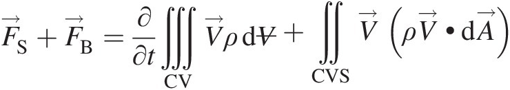 (2.56)
where ΠS=F→S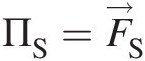 and ΠB=F→B
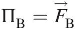 , which are surface and body forces, respectively, and ϕ=V→
 is the intensive property corresponding to the linear momentum M→
 . Surface forces arising from the static pressure at inlets, outlets, and walls of a control volume are compressive in nature, being always normal to the surface. Wall shear stresses, which also contribute to the surface forces, are locally parallel to the surface. In this text, we consider only two kinds of body forces, one as a result of gravity (weight) and the other as a result of rotation (centrifugal force).
It is instructive to analyze Equation 2.56 as three independent equations, one for each coordinate direction of a Cartesian coordinate system. This is possible because the forces acting along one coordinate direction will not change the momentum in the other coordinate direction, which is orthogonal. Accordingly, for the following presentation, let us only consider the xx component of Equation 2.56 in an assigned Cartesian coordinate system:
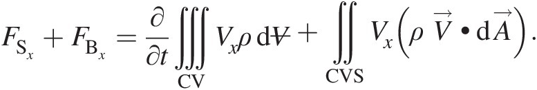 (2.57)
If the velocity, static pressure, and density are uniform at each inlet and outlet of a control volume, we can replace the surface integral on the right-hand of Equation 2.57 by algebraic summations. For a control volume with NiNi inlets and NjNj outlets having MxMx as its total instantaneous value of xx momentum, Equation 2.57 simplifies to
 (2.58)
where
Vxi≡Vxi≡ xx-momentum velocity at inlet i
Vxj≡Vxj≡ xx-momentum velocity at outlet j
ṁi≡
 Mass flow rate at inlet i (ṁi=ρiAiVi
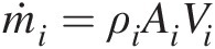 )
)
ṁj≡
 Mass flow rate at outlet j (ṁj=ρjAjVj
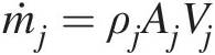 )
)


For an inertial (nonaccelerating) control volume, Equation 2.58 reads the following:
(Sum of surface forces: pressure force and shear force)
+ (Sum of body forces: gravitational force and centrifugal force under rotation)
= (Time-rate of change of xx-momentum within the control volume)
+ (Total xx-momentum flow rate leaving the control volume)
– (Total x-momentum flow rate entering the control volume)
In Equation 2.58, ViVi and VjVj are the mass velocity at each inlet and outlet, respectively. They are always positive and independent of the chosen coordinate system. By contrast, VxiVxi and VxjVxj are the xx-momentum velocity at inlet i and outlet j, respectively. Whether they are positive or negative is determined relative to the positive direction of the chosen coordinate system. Identifying mass velocity (the velocity that produces mass flow rate) and momentum velocity (the velocity component for which the linear momentum equation is being considered) greatly simplifies the evaluation of the momentum flow rate with the correct sign at each inlet and outlet of a control volume.
To demonstrate the use of mass velocity and momentum velocity in the control volume analysis of linear momentum, let us consider a steady flow through the control volume shown in Figure 2.6. Based on the direction of each flow velocity, it is easy to see that sections 2 and 3 are inlets and sections 1, 4, and 5 are outlets. The mass velocity and xx-momentum velocity for each inlet and outlet are summarized in Table 2.1. Note that, with reference to the Cartesian coordinate system shown in the figure, the xx-momentum velocities for inlet 3 and outlet 1 are negative. For outlet 5, whereas the mass velocity V5V5 in the yy direction is nonzero, the corresponding xx-momentum velocity is zero. With various quantities given in Table 2.1 for a steady flow through the control volume, the right-hand side of Equation 2.58 can be easily evaluated.

Figure 2.6 A control volume showing flow properties at its two inlets and three outlets.
Table 2.1 xx-Momentum Flow Rate and Stream Thrust at Each Inlet and Outlet of the Control Volume of Figure 2.6
| Inlet/ Outlet | Mass Velocity | Mass Flow Rate | x-Momentum Velocity | x-Momentum Flow Rate | Stream Thrust |
|---|---|---|---|---|---|
| 1 (outlet) | V1V1 | ṁ1=ρ1A1V1 | −V1−V1 | −ṁ1V1 | −ṁ1V1+Ps1A1 |
| 2 (inlet) | V2V2 | ṁ2=ρ2A2V2 | V2V2 | ṁ2V2 | ṁ2V2+Ps2A2 |
| 3 (inlet) | V3V3 | ṁ3=ρ3A3V3 | −V3−V3 | −ṁ3V3 | −ṁ3V3+Ps3A3 |
| 4 (outlet) | V4V4 | ṁ4=ρ4A4V4 | V4V4 | ṁ4V4 | ṁ4V4+Ps4A4 |
| 5 (outlet) | V5V5 | ṁ5=ρ5A5V5 | 00 | 00 | 00 |
If we separate out the pressure force at each inlet and outlet of the control volume from the total surface forces F→S on the left-hand side of Equation 2.58, and combine it with the corresponding momentum flow on the right-hand side of the equation, we can express the momentum equation in terms of stream thrust in the xx direction. In Table 2.1, note that the stream thrust at each inlet and outlet has the same sign as the momentum velocity.
How to handle nonuniform flow properties at inlets and outlets and to express the linear momentum equation in a noninertial (accelerating or decelerating) reference frame attached to the control volume are discussed in comprehensive details by Sultanian (2015).
2.2.6.3 Angular Momentum Equation
Because angular momentum is expressed as H→=r→×M→ , the angular momentum equation is not a new conservation law, but simply a moment of the linear momentum equation. In word form, the angular momentum equation can be expressed as
(Sum of the torque from surface forces: pressure force and shear force)
+ (Sum of the torque from body forces: gravitational force and centrifugal force)
= (Time-rate of change of angular momentum within the control volume)
+ (Total angular momentum flow rate leaving the control volume)
– (Total angular momentum flow rate entering the control volume)
In equation form, we can write the aforementioned statement in an inertial coordinate system as
 (2.58)
Similar to the approach presented in the previous section for the evaluation of linear momentum flow at an inlet or outlet of a control volume by using the concept of mass velocity and momentum velocity, we can evaluate each angular momentum flow rate by taking the product of mass velocity and angular momentum, which is considered positive in the counterclockwise direction and negative in the clockwise direction. Table 2.2 summarizes the flow rate of zz-component of the angular momentum for each inlet and outlet of the control volume shown in Figure 2.6, demonstrating the application of the approach proposed here.
Table 2.2 z-Component Angular Momentum Flow Rates at Inlets and Outlets of the Control Volume of Figure 2.6
| Inlet / Outlet | Mass velocity | Specific z-component angular momentum | z-component angular momentum flow rate |
|---|---|---|---|
| 1 (outlet) | V1V1 | a1V1a1V1 | a1V1(ρ1A1V1)a1V1ρ1A1V1 |
| 2 (inlet) | V2V2 | a2V2a2V2 | a2V2(ρ2A2V2)a2V2ρ2A2V2 |
| 3 (inlet) | V3V3 | −a3V3−a3V3 | −a3V3(ρ3A3V3)−a3V3ρ3A3V3 |
| 4 (outlet) | V4V4 | −a4V4−a4V4 | −a4V4(ρ4A4V4)−a4V4ρ4A4V4 |
| 5 (outlet) | V5V5 | b5V5b5V5 | b5V5(ρ5A5V5)b5V5ρ5A5V5 |
A coordinate system rotating at constant angular velocity is considered noninertial. In this noninertial coordinate system with no linear and rotational accelerations, we can write, see Sultanian (2015), the integral angular momentum equation for a control volume as
 (2.59)
where Ω→ is the constant speed of rotation and the relative velocity W→
 is the flow velocity in this coordinate system with its corresponding value in the stationary (inertial) coordinate system represented by the absolute V→
 . Note that expressing the linear momentum equation in this noninertial coordinate system gives rise two new terms: the Coriolis acceleration term 2Ω→×W→
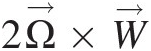 and the centrifugal acceleration term Ω→×(Ω→×r→)
 , whose moments appear in Equation 2.59.
For turbomachinery flows, including those in a gas turbine with a single axis of rotation, a cylindrical coordinate system shown in Figure 2.7 is a natural choice. In this coordinate system, the axial coordinate direction is aligned with the axis of rotation. As shown in the figure, the tangential direction is perpendicular to the meridional plane, which is formed by the axial and radial directions. For a constant rotational speed ΩΩ and steady flow, Sultanian (2015) presents a mathematically rigorous simplification of Equation 2.59 to yield
 (2.60)
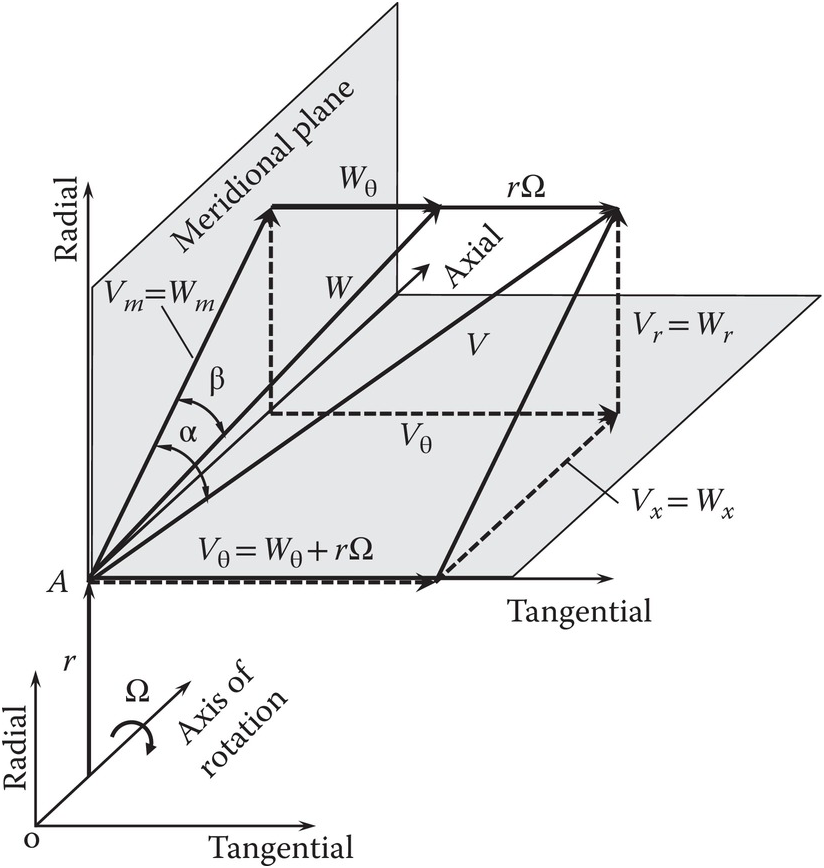
Figure 2.7 Cylindrical coordinate system used in turbomachinery flows.
In the derivation of Equation 2.60 from Equation 2.59, it is seen that the moment of the centrifugal force term makes no contribution and the volume integral of the moment of the Coriolis term contributes to the surface integral and converts the flow of angular momentum in the noninertial reference into that in the inertial reference frame at each inlet and outlet of the control volume. Equation 2.60 involves only the tangential velocity VθVθ in the inertial reference frame, forming the basis for the Euler’s turbomachinery equation discussed in Section 2.2.8.
With reference to Figure 2.7, we see that the angular momentum vector at point AA in the flow about the turbomachinery axis of rotation is the cross-product of the radial vector r→ and the velocity vector V→
 . Because the radial velocity VrVr is collinear with the radial vector, its contribution to angular momentum will be zero. The contribution of axial velocity VxVx to angular momentum will be in the tangential direction and not along the axis of rotation. Thus, only the tangential velocity VθVθ contributes to the angular momentum vector along the rotation axis, giving the angular momentum flow rate Ḣx=ṁrVθ
 .
.
For uniform properties at control volume inlets and outlets, we can replace the surface integral in Equation 2.60 by algebraic summations, giving
 (2.61)
2.2.6.4 Energy Equation
The energy equation embodies the first law of thermodynamics. According to Equation 2.1, heat transfer and work transfer are the agents responsible for change in the total energy of a system. Thus, with ϕ = e = u + V2/2 + gzϕ=e=u+V2/2+gz as the intensive property corresponding to the total energy EE, Equation 2.51 for the energy conservation becomes
 (2.62)
In Equation 2.62, according to the convention used in Equation 2.1, the work transfer into the control volume becomes negative. Recognizing different types of work transfer into the control volume, we can write this equation as
 (2.63)
where
Q̇≡
 Rate of heat transfer into the control volume through its control surface
Ẇpressure≡
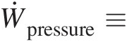 Rate of work transfer into the control volume by pressure force
Ẇshear≡
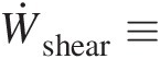 Rate of work transfer into the control volume by shear force
Ẇrotation≡
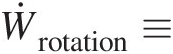 Rate of Euler work transfer into the control volume by rotation
Ẇshaft≡
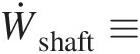 Rate of shaft work into the control volume
Ẇother≡
 Rate of other energy transfers into the control volume: chemical energy, electrical energy, electromagnetic energy, and so on.


In a nondeformable control volume, the pressure force can do work only at its inflows and outflows. Within the control volume itself, the pressure force at any point has an equal and opposite pressure force, and does not contribute to the work transfer term Ẇpressure . At an inlet to the control volume, because V→
 and A→
 are in opposite direction, ρV⇀⋅dA⇀
 will be negative, and the pressure force will do work on the flow entering the control volume.
According to our convention, we express the work transfer by the pressure force at inlets as

At control volume outlets, ρV⇀⋅dA⇀ is positive, and the pressure force opposes the flow exiting the control volume. We can thus write

Combining the aforementioned two equations, we can express Ẇpressure by the following surface integral, which is true at all inlets and outlets:

where Ps/ρPs/ρ is the specific flow work.
Transferring Ẇpressure to the right-hand side of Equation 2.63 yields
 (2.64)
Replacing u + Ps/ρu+Ps/ρ by the specific static enthalpy hshs in Equation 2.64, we obtain
 (2.65)
For uniform properties at control volume inlets and outlets, we can replace the surface integral in Equation 2.65 by algebraic summations, giving
 (2.66)
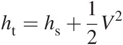
Note that, in Equation 2.66, we can further combine the specific static enthalpy hshs and specific kinetic energy V2/2V2/2 to yield the specific total enthalpy ht = hs + V2/2ht=hs+V2/2.
2.2.6.5 Entropy Equation
The entropy equation is founded in the second law of thermodynamics, which states that the entropy of an isolated system increases if the processes within the system are irreversible; the entropy remains constant when the processes are reversible. By introducing the concept of entropy production as a change agent, in addition to the change in entropy as a result of heat transfer, we can write Equation 2.51 for entropy as
 (2.67)
where ϕ = sϕ=s is the entropy per unit mass. In this equation, the rate of entropy production Ṗentropy accounts for entropy generation within the control volume from all irreversible processes and Q̇
 is the rate of heat transfer into the control volume through its surface at temperature TT.
The unsteady integral term on the right-hand side of Equation 2.67 is the rate of storage of entropy within the control volume and should not be confused with Ṗentropy , which represents the rate of entropy production associated with the irreversibility of energy transfer into the control volume. For the case with no heat transfer, Ṗentropy
 equals the rate of increase in entropy stored within the control volume plus the excess of the entropy outflow rate over its inflow rate through the control-volume surface. Further note that there is no counterpart to Ṗentropy
 in the equations of mass, momentum, and energy whose conservation laws dictate zero production within the control volume.
In a steady flow, the unsteady integral term in Equation 2.67 vanishes, yielding Equation 2.68 in which Ṗentropy and other terms are considered time-independent.
 (2.68)
For uniform properties at control volume inlets and outlets, we can again replace the surface integral in Equation 2.68 by algebraic summations, giving
 (2.69)
2.2.7 Euler’s Turbomachinery Equation
Euler’s turbomachinery equation is widely used in all types of turbomachinery. This equation, derived from the angular momentum equation discussed in Section 2.2.5.3, determines power transfer between the fluid and the rotor blades. In pumps, fans, and compressors, the power transfer occurs into the fluid to increase its outflow rate of angular momentum over the inflow rate; in turbines, the power transfer occurs to the rotor from the fluid to decrease its outflow rate of angular momentum over the inflow rate. The power transfer to or from the fluid is simply the product of the torque and rotor angular velocity in radians per second.
Let’s consider a steady adiabatic flow in a rotating passage between two blades of a mixed axial-radial-flow turbomachinery, as shown in Figure 2.8. Each of the velocity vectors, V→1 at the inlet 1 and V→2
 at outlet 2, has components in axial, radial, and tangential directions. The meridional velocity, which is the resultant of the axial and the radial velocities, is the mass velocity in the rotating passage flow at sections 1 and 2. Let Vθ1Vθ1 be the tangential velocity at inlet 1 and Vθ2Vθ2 at outlet 2. For a constant mass flow rate ṁ
 through the rotating passage, the angular momentum equation, Equation 2.61, yields
 (2.70)
Figure 2.8 Flow through an axial-radial-flow turbomachinery passage between adjacent blades.
The aerodynamic power transfer, which is the rate of work transfer as a result of the aerodynamic torque acting on the fluid control volume, is given by
 (2.71)
where U1U1 and U2U2 are rotor tangential velocities at inlet 1 and outlet 2, respectively. Using steady flow energy equation in terms of total enthalpy at sections 1 and 2, we can also write
 (2.72)
Combining Equations 2.71 and 2.72 yields
Equation (2.73) is known as the Euler’s turbomachinery equation. This equation simply states that, under adiabatic conditions, the change in specific total enthalpy of the fluid flow between any two sections of a rotor equals the difference in the products of the rotor tangential velocity and flow tangential velocity at these sections. This equation further reveals that for turbines, where the work is done by the fluid, we have ht2 < ht1ht2<ht1 and U2Vθ2 < U1Vθ1U2Vθ2<U1Vθ1; and for compressors, fans, and pumps, where the work is done on the fluid, we have ht2>ht1ht2>ht1 and U2Vθ2>U1Vθ1U2Vθ2>U1Vθ1.
For axial flow machines, where r1≈r2r1≈r2 and U1≈U2U1≈U2, Equation 2.73 reveals that the change in total enthalpy is entirely as a result of the change in the flow tangential velocity, that is, Δht=U¯ΔVθ , requiring blades with camber (bow). By contrast, for radial machines (radial turbines and centrifugal compressors), the change in total enthalpy results largely as a result of the change in rotor tangential velocity as a result of the change in radius, that is, Δht=ΔUV¯θ
 .
.
2.2.7.1 Rothalpy
The concept of rothalpy is grounded in Euler’s turbomachinery equation presented in the preceding section. Rearranging Equation 2.73 yields
which reveals that the quantity (ht − UVθ)ht−UVθ at any point in a rotor flow remains constant under adiabatic conditions (no heat transfer). This quantity is called rothalpy expressed as
 (2.75)
where both htht and VθVθ are in the inertial (stationary) reference frame. Let us now convert Equation 2.75 into the rotor reference frame. If VxVx, VrVr, and VθVθ are, respectively, the axial, radial, and tangential velocity components of the absolute velocity V→ at any point in the flow; and similarly, if WxWx, WrWr, and WθWθ are, respectively, the axial, radial, and tangential velocity components of the corresponding relative velocity W→
 at that point, we can write the following equations:
 (2.76)
 (2.77)
where UU is the local tangential velocity of the rotor. Substituting for VθVθ from Equation 2.78 into Equation 2.76 and noting that Wx = VxWx=Vx and Wr = VrWr=Vr, we obtain
 (2.79)
Using Equations 2.78 and 2.79, we rewrite Equation 2.75 as

which simplifies to
 (2.80)
where htRhtR is the specific total enthalpy in the rotor reference frame. Equation 2.80 yields an interesting interpretation of rothalpy in a rotating system in that the change in fluid relative total enthalpy between any two radii in this system equals, under adiabatic conditions, the change in dynamic enthalpy associated with the solid-body rotation over these radii.
For a calorically perfect gas (constant cpcp), we can also write Equation 2.80 as
 (2.81)
where TtRTtR is the fluid total temperature in the rotor reference frame.
2.2.7.2 An Alternate Form of the Euler’s Turbomachinery Equation
For an adiabatic flow in a rotor, the rothalpy remains constant, that is, I1 = I2I1=I2. Using Equation 2.80 we can write
 (2.82)
Equation 2.82 expresses the change in fluid static enthalpy in a rotor in terms of changes in the flow relative velocity and rotor tangential velocity. From the definition of total enthalpy, we can write its change between locations 1 and 2 as
 (2.83)
Using Equation 2.82 to substitute for (hs2 − hs1)hs2−hs1 in Equation 2.83 yields the following alternate form of Euler’s turbomachinery equation earlier derived as Equation 2.73:
 (2.84)
where the terms on the right-hand side have the following physical interpretations:


2.2.7.3 Total Pressure and Total Temperature in Stator and Rotor Reference Frames
In turbomachinery, we need to consider flow properties in both stator (absolute, stationary, or inertial) and rotor (relative, rotating, or noninertial) reference frames. Because turbomachinery generally has a single axis of rotation, tangential (swirl) velocity is the only velocity component that is impacted by the change of reference frames from stator to rotor or vice versa. Both the axial and radial velocity components do not change. Further, all static properties of the fluid; for example, the static temperature and static pressure, remain the same in both stator and rotor reference frames.
Total temperature in both incompressible and compressible flows is computed by the equations:
 (2.85)
 (2.86)
In an incompressible flow (constant density), the total pressure is evaluated by the equations:
 (2.87)
 (2.88)
In a compressible flow, an isentropic stagnation process is assumed to obtain total properties. Accordingly, we invoke the isentropic relations to compute the total pressure using the following equations in each reference frame:
 (2.89)
 (2.90)
Conversion from stator reference frame to rotor reference frame. Tangential velocities in the two reference frames are related by Equation 2.78, giving Wθ = Vθ − UWθ=Vθ−U. Because the fluid static temperature remains invariant in both reference frames, we can write
 (2.91)
Because Wx = VxWx=Vx and Wr = VrWr=Vr, Equation 2.91 reduces to
 (2.92)
Substituting Wθ = Vθ − UWθ=Vθ−U in Equation 2.92, we obtain
 (2.93)
which yields TtR = TtSTtR=TtS for Vθ = U/2Vθ=U/2.
For an isentropic compressible flow, we can use Equation 2.93 to obtain the pressure ratio as
 (2.94)
Conversion from rotor reference frame to stator reference frame. Using Equation 2.78 to substitute for VθVθ in Equation 2.93, and rearranging terms, we obtain
 (2.95)
 (2.96)
which uses the fact that both the static pressure and static temperature, being fluid state properties, are independent of the reference frame. Equation 2.96 thus gives
 (2.97)
An easier approach to first converting total temperatures, and then total pressures, between stator and rotor reference frames is by equating the expressions of rothalpy in these reference frames, as given by Equations 2.75 (I = cpTtS − UVθI=cpTtS−UVθ) and 2.81 (I = cpTtR − U2/2I=cpTtR−U2/2) and converting tangential velocities in these reference frames by using Equation 2.78.
2.2.8 Compressible Flow with Area Change, Friction, Heat Transfer, Rotation, and Normal Shocks
Compressible flows are ubiquitous in gas turbines. The key parameter that characterizes a compressible flow is its Mach number (M = V/CM=V/C), which is the ratio of the flow velocity to speed of sound (C=κRTs ). For M ≤ 0.3M≤0.3, the gas flow may be treated as incompressible for most practical engineering calculations using a constant density, which is obtained using the perfect gas law Ps/ρ = RTsPs/ρ=RTs. With several examples from gas turbine design applications, Sultanian (2015) presents comprehensive details of compressible flows with area change, friction, heat transfer, rotation, normal, and oblique shocks. In our presentation of internal compressible flows in this section, all the flow properties are uniform to be uniform at each section.
Let us briefly reflect on the fundamental difference between a compressible flow and an incompressible flow with constant density. The total energy of a flow, as measured by its total temperature, is the sum of the fluid static temperature, which is the average kinetic energy associated with the gas molecules, and the dynamic temperature based on the flow kinetic energy. In an incompressible flow, there is negligible coupling between the external flow energy and its internal one. For example, when water flows through a converging-diverging (C-D) nozzle with constant entropy (constant total pressure and total temperature), the throat section with its minimum area features the maximum flow velocity, or the flow kinetic energy, with negligible decrease in its static temperature, a measure of the internal energy of the flow. Note that the specific heat of water is more than four times that of air. Further, in an incompressible flow, total pressure (Pt = Ps + ρV2/2Pt=Ps+ρV2/2) may be interpreted as the total mechanical energy per unit volume of the flow. The constancy of total pressure in an ideal incompressible flow leads to the famous Bernoulli equation with its tenet of “high velocity, low pressure” at any point in the flow.
A compressible flow, by contrast, exhibits quite different characteristics, particularly at high Mach numbers. For an isentropic airflow in a choked C-D nozzle with exit pressure ratio (ratio of total-to-static pressure) of more than two, both the static pressure and static temperature continuously decrease in the flow direction with continuous increase in Mach number. In the diverging section with increasing flow area, Mach number increases mainly as a result of the increase in the flow velocity needed to maintain a constant mass flow rate through the nozzle under significantly decreasing density. This behavior is somewhat counterintuitive based on our understanding of an incompressible internal flow where, for a given mass flow rate, the flow velocity always decreases with increasing area.
Note that the square of Mach number indicates the ratio of the external energy to internal energy of the flow. This provides a useful physical insight into Mach number. When the airflow expands in a C-D nozzle, increasing Mach number entails increase in the external flow energy and decrease in the internal one, the total flow energy remaining constant (constant total temperature). In other words, the change in Mach number is associated of the exchange between the internal flow energy and external flow energy. This two-way coupling between the internal and external flow energies in a compressible flow, also known as the compressibility effect, makes it fundamentally different from an incompressible flow. Note that the compressibility effect increases with Mach number. At low Mach numbers (M ≤ 0.3M≤0.3), as stated before, the compressibility effect may be neglected, and the compressible flow may be assumed to behave like an incompressible flow. On the other hand, an incompressible flow cannot be modeled to behave like a compressible flow. Based on this discussion, one should therefore avoid the use of Bernoulli equation or its extended form, also called the mechanical energy equation, in a compressible flow.
The phenomenon of choking is again unique to a compressible flow. At any section of fixed area, when the Mach number is unity (M = 1M=1), the flow is considered to be choked at that section, meaning the downstream changes in the pressure boundary condition will have no effect on the mass flow rate through the section. Note, however, that this maximum mass flow rate can still be changed by changing the upstream boundary conditions where the flow is subsonic (M < 1M<1). Choking has a simple physical interpretation. Because small pressure changes in a gas travel at the speed of sound in all directions, for M = 1M=1 at a section, the flow velocity equals the local speed of sound and prevents any sound wave to travel upstream of this section. As a result, the lowering of the C-D nozzle exit static pressure, after it is choked at the throat, will not flow more regardless of how much we decrease this pressure as long as the upstream total pressure and total temperature remain constant.
2.2.8.1 Isentropic Flow
Isentropic gas flows are hard to find in a real word, including gas turbines. Nevertheless, these flows serve as ideal reference flows in many design applications. From Equation 2.17, we obtain the following relation between the pressure ratio and temperature ratio at two points of an isentropic compressible flow:
 (2.98)
Because the stagnation process in a compressible flow is assumed isentropic, a practical application of Equation 2.98 is to compute the maximum local stagnation pressure using the equation
 (2.99)
where the total temperature is computed as Tt = Ts + 0.5V2/cpTt=Ts+0.5V2/cp. It is often convenient to express compressible flow equations in terms of Mach number. These equations for an isentropic compressible flow are summarized in Table 2.3.


2.2.8.2 Mass Flow Functions
In an internal flow, mass flow rate is simply calculated as ṁ=ρAV , where the velocity VV is normal to the flow area AA. In steady state, regardless of changes in density, area, and velocity, the mass flow rate remains constant at each section. Further, for an incompressible flow and subsonic compressible flow in a duct, the exit static pressure must always equal the ambient static pressure, which acts as the discharge pressure boundary condition. In our approach in this textbook, we use only the properties at a section to compute mass flow rate at that section. For the flow to occur in either direction at a section, the total pressure at the section must be greater than the static pressure. Discounting the change in entropy as a result of heat transfer, an internal flow at any section occurs in the direction of increasing entropy.
In a compressible flow, the mass flow functions provide a convenient means of computing mass flow rate at a section without explicitly using the fluid density, which does not remain constant in such a flow. This approach is widely used by design engineers in the gas turbine industry. Starting with the equation ṁ=ρAV and using the isentropic flow equations along with the equation of state (Ps/ρ = RTsPs/ρ=RTs), we can easily express the mass flow rate at a section as
 (2.100)
where F̂fs is the dimensionless static-pressure mass flow function given by
 (2.101)
and FfsFfs, having the dimensions of 1/R , is the static-pressure mass flow function given by
 (2.102)
Note that, for a calorically perfect gas, both F̂fs and FfsFfs are functions of Mach number only.
Equation 2.100 shows that, for a given Mach number, the mass flow rate at a section is proportional to the static pressure and inversely proportional to the square root of the total temperature. Both the static pressure and total temperature are assumed to be uniform over that section.
Using Pt/PsPt/Ps in terms of Mach number from Table 2.3, we can replace PsPs in Equation 2.100 by PtPt and alternatively express the mass flow rate as
 (2.103)
where F̂ft is the dimensionless total-pressure mass flow function given by
 (2.104)
and FftFft, having the dimensions of R , is the total-pressure mass flow function given by
 (2.105)
For a calorically perfect gas both F̂ft and FftFft are functions of Mach number only.
Equation 2.103 shows that, for a given Mach number, the mass flow rate at a section is proportional to the total pressure and inversely proportional to the square root of the total temperature. Both the total pressure and total temperature are assumed to be uniform over that section.
Figure 2.9 shows the variations of mass flow functions F̂ft and F̂fs
 with Mach number for κ = 1.4κ=1.4. As shown in the figure, F̂ft
 increases as Mach number increases for M < 1M<1 (subsonic flow) and decreases as Mach number increases for M>1M>1 (supersonic flow), and it has a maximum value of 0.6847 at M = 1M=1(sonic flow), which corresponds to the choked flow conditions at the flow area. For example, for the ambient air at 20°C20°C and 1.013 bar1.013bar, Equation 2.103 computes 239.2 kg/s239.2kg/s as the maximum possible mass flow rate through an area of 1.0 m21.0m2. Furthermore, the figure shows that each value of Mach number yields a single value of mass flow function F̂ft
 , but each value of flow function F̂ft
 corresponds to two values (except at M = 1M=1) of Mach number – one subsonic and the other supersonic. While the calculation of F̂ft
 by Equation 2.103 for a given value of Mach number is direct, we need to use an iterative method (e.g., “Goal Seek” in MS Excel) to compute subsonic and supersonic Mach numbers for a given value of F̂ft
 .
.

Figure 2.9 Variations of mass flow functions F̂ft and F̂fs
 with Mach number for κ = 1.4κ=1.4.
As shown in Figure 2.9, unlike F̂ft , F̂fs
 increases monotonically with Mach number without exhibiting a maximum value at M = 1M=1, implying one-to-one correspondence between F̂fs
 and MM. Note that the ratio F̂fs/F̂ft
 equals the total-to-static pressure ratio Pt/PsPt/Ps, which increases monotonically with Mach number, more rapidly for M>1M>1. For a given value of F̂fs
 , we present here a direct method to calculate the corresponding Mach number.
Finding Mach number for a given static-pressure mass flow function. Squaring both sides of Equation 2.101, we obtain


which is a quadratic equation in M2M2 with the positive root given by
 (2.106)
Use of isentropic flow tables to compute mass flow functions. Not all isentropic flow tables list mass flow functions; however, they all list quantities like pressure ratio Pt/PsPt/Ps and area ratio A/A∗A/A∗ against Mach number. For an isentropic flow, we know that the total pressure and total temperature remain constant in a variable-area duct. In a duct flow, we can equate the mass flow rate at a give section of area AA to that at the sonic throat area A∗A∗(imaginary if it is outside the duct), giving
 (2.107)
and
 (2.108)
Knowing the Mach number at a section, we can look up Pt/PsPt/Ps and A/A∗A/A∗ in isentropic flow tables; then use Equation 2.107 to compute F̂ft , followed by Equation 2.108 to compute F̂fs
 at that section.
2.2.8.3 Impulse Functions
As discussed in Section 2.2.5, the concept of stream thrust is grounded in the linear momentum equation. The change in stream thrust (the total stream thrust at outflows minus the total stream thrust at inflows) across a duct represents the total thrust on a duct as a result of fluid flow.
Using impulse functions, we can express the stream thrust at any section of a compressible duct flow as
where IfsIfs is the static-pressure impulse function given by
and IftIft is the total-pressure impulse function given by
 (2.111)
Note that the ratio Ifs/IftIfs/Ift equals the total-to-static pressure ratio Pt/PsPt/Ps. For a given gas flow, both IfsIfs and IftIft are functions of Mach number only.
Figure 2.10 shows the monotonically increasing parabolic variation of IfsIfs with Mach number for κ = 1.4κ=1.4. As shown in the figure, IfsIfs increases with MM for M < 1M<1, has a maximum value of 1.2679 at M = 1M=1, and decreases with MM for M>1M>1.

Figure 2.10 Variations of impulse functions IftIft and IfsIfs with Mach number for κ = 1.4κ=1.4.
2.2.8.4 Normal Shock Function
When a supersonic compressible flow needs to adjust to a sudden increase in downstream static pressure, it undergoes a normal shock, which is a very thin nonequilibrium region featuring an abrupt increase in entropy, while its total temperature and mass flow rate remain constant. The flow upstream of a normal shock is always supersonic and the downstream flow always subsonic. Thus, the static temperature across a normal shock increases, and the flow velocity decreases with simultaneous increase in density to satisfy continuity.
Let us consider a constant-area control volume simulating a normal shock under the boundary conditions of no heat transfer and surface force. In this case, therefore, the mass flow rate, the stream thrust, and the total temperature over the control volume all remain constant. Thus, the ratio of mass flow rate to stream thrust at the inlet (upstream of the normal shock) and outlet (downstream of the normal shock) of our control volume must be equal. Evaluating this ratio using Equations 2.103 and 2.109 yields

The aforementioned equation reveals that the ratio F̂ft/Ift must remain constant across a normal shock. We call this ratio, which is the ratio of total-pressure mass flow function to the total-pressure impulse function, the normal shock function NN expressed as the following function of MM and κκ:
 (2.112)
For M = 1M=1, Equation 2.112 yields
 (2.113)
which for κ = 1.4κ=1.4 equals 0.540. For M→∞M→∞, Equation 2.112 yields N∞N∞ as
 (2.114)
For κ = 1.4κ=1.4 we obtain N∞ = 0.378N∞=0.378. It is interesting to note that the corresponding value of the subsonic Mach number is also equal to 0.378. This can be easily demonstrated by substituting M=κ−1/2κ in Equation 2.112 and obtaining N=κ−1/2κ
 after some simplification of the right-hand of the equation. From this we can conclude that, even for the strongest normal shock, the downstream subsonic Mach number will not be lower than κ−1/2κ
 .
.
The behavior of the normal shock function NN as a function of Mach number is depicted in Figure 2.11 for κ = 1.4κ=1.4. Like the total-pressure mass flow function F̂ft and the total-pressure impulse function IftIft, the figure shows that NN also increases with MM for M < 1M<1, reaches a maximum value of N∗ = 0.540N∗=0.540 at M = 1M=1, and decreases with MM for M>1M>1.

Figure 2.11 Variation of normal shock function NN with Mach number for κ = 1.4κ=1.4.
In addition to simplifying the computations of compressible flows without the explicit use of density, the mass flow functions, impulse functions, and normal shock function presented in the foregoing sections are very helpful in explaining many seemingly nonintuitive behaviors these flows, as we will see in the following sections.
2.2.8.5 Isentropic Flow with Area Change
For the differential control volumes for mass conservation, force-momentum balance, and energy conservation shown in Figure 2.12, Sultanian (2015) presents a detailed derivation of the following differential equation for flow velocity change under the influence of area change, friction, heat transfer, and rotation:
 (2.115)
where the rotational Mach number Mθ=rΩ/κRTs . Being nonlinear, Equation 2.115 generally requires a numerical solution when all effects are presents, as in a serpentine passage used in internal cooling of gas turbine blades (with rotation) and vanes (without rotation).

Figure 2.12 Differential control volumes: (a) mass, (b) linear momentum, and (c) energy.
To develop a good intuitive understanding of a compressible duct flow, let us consider one effect at a time. For an isentropic compressible flow in a variable-area duct, Equation 2.115 reduces to
 (2.116)
which clearly shows that, for subsonic (M < 1M<1) flows with the coefficient (1 − M21−M2) being positive, the flow velocity increases as the duct area decreases and vice versa. For supersonic (M>1M>1) flows; however, the coefficient (1 − M21−M2) being negative, the flow velocity increases with duct area and vice versa. As discussed earlier, a supersonic C-D nozzle used in rocket engines features this counterintuitive compressible flow behavior.
2.2.8.6 Isentropic Flow with Rotation
For an isentropic flow in a constant-area duct rotating around an axis other than along the flow direction, Equation 2.115 reduces to
 (2.117)
Note that the duct rotation essentially effect the flow in two ways; first, as a body force (centrifugal force) in the momentum equation, and second, as rotational work transfer in the energy equation. For the velocity change in the flow, both these effects are combined into the term on the right-hand side of Equation 2.117.
Because Mθ2 is positive definite, Equation 2.117 reveals that, for a subsonic flow, the velocity will increase when the flow is radially inward (dr < 0dr<0) and decrease when the flow is radially outward (dr>0dr>0). When the flow is supersonic in a constant-area rotating duct flow, it will exhibit the opposite behavior.
2.2.8.7 Nonisentropic Flow with Friction: Fanno Flow
The nonisentropic compressible flow with friction in a constant-area duct with no rotation and no heat transfer is known as Fanno flow. In this case, Equation 2.115 reduces to
 (2.118)
Because the right-hand side of Equation 2.118 is always positive, we infer from this equation that the friction will always accelerate a subsonic flow and decelerate a supersonic flow. The fact that the friction accelerates a subsonic flow in a constant-area duct is counterintuitive to our experience on the effects of friction, which is known to slow things down.
A simple physics-based reasoning behind why the flow accelerates in a subsonic Fanno flow, in which the total temperature, flow area, and mass flow rate remain constant, runs as follows. For the flow to overcome wall shear force as a result of friction, which always opposes the flow, we need a net pressure force in the flow direction. This entails that the static pressure and density (from the equation of state) decrease downstream. Because the duct area remains constant, the flow velocity must increase to maintain the constant mass flow rate.
Another way to explain the flow behavior in a Fanno flow is through the continuity equation expressed in terms of the total-pressure mass flow function, Equation 2.103. The effect of friction in an adiabatic flow is always to increase entropy and decrease total pressure in the flow direction. Because the mass flow rate at each section of a steady internal flow remains constant, Equation 2.103 dictates that the downstream total-pressure mass flow function (F̂ft ) must increase in the flow direction. According to the variation of F̂ft
 with Mach number shown in Figure 2.9, it is clear that the downstream Mach number should move closer toward the sonic condition (M = 1M=1). This explains why in a Fanno flow the downstream Mach number increases if the flow is subsonic and decreases if it is supersonic. This reasoning can also be extended to conclude that the exit Mach number of a Fanno flow is limited to M = 1M=1(frictional choking) for both subsonic and supersonic flows at the inlet.
Table 2.4 summarizes a set of equations to evaluate changes in various properties in a Fanno flow. Detailed derivations of these equations are given by Sultanian (2015).
Table 2.4 Fanno Flow Equations
TsTs∗=κ+12+κ−1M2  | ρρ∗=1M2+κ−1M2κ+1  | PsPs∗=1Mκ+12+κ−1M2  |
PtPt∗=1M2+κ−1M2κ+1κ+12κ−1  | PiPi∗=Ps1+κM2Ps∗κ+1  | |
fLmaxDh=κ+12κlnκ+1M22+κ−1M2+1κ1M2−1  | ||
2.2.8.8 Nonisentropic Flow with Heat Transfer: Rayleigh Flow
The nonisentropic compressible flow in a nonrotating, constant-area, frictionless duct with heat transfer (both heating and cooling of the flow) is known as Rayleigh flow. Because friction is always present in real duct flows, Rayleigh flows are seldom found in engineering applications. Nevertheless, it is instructive to study these flows to develop a better understanding of the effects of heat transfer. The following reduced form of Equation 2.115 shows that the heating will increase flow velocity for a subsonic Rayleigh flow (M < 1M<1) and will decrease it for a supersonic Rayleigh flow (M>1M>1). In addition, this equation also shows that cooling the flow will have opposite trends in velocity changes in the flow direction.
 (2.119)
In a Rayleigh flow, in addition to the area and mass flow rate, the stream thrust (zero shear force from the wall) remains constant at each section. Combining Equations 2.103 and 2.109, we can express the stream thrust as
 (2.120)
If the upstream and downstream sections of a Rayleigh flow are designated by subscripts 1 and 2, respectively, we have ST1 = ST2ST1=ST2, which according to Equation 2.120 yields

For heating, we have Tt2>Tt1Tt2>Tt1, which means N2>N1N2>N1. According to the variation of NN with Mach number shown in Figure 2.11, we further conclude that M2M2 should be closer to M = 1M=1 than to M1M1. In other words, if the upstream flow is subsonic, the Mach number will increase downstream. By contrast, if the flow is supersonic, the Mach number will decrease downstream. Thus, heating in a Rayleigh flow raises a subsonic Mach number and lowers a supersonic Mach number toward the sonic condition (thermal choking).
From the constancy of stream thrust between any two sections of a Rayleigh flow, we can write
 (2.121)
Based on the dependence of IftIft on Mach number shown in Figure 2.10, because M2M2 is on the same side as M1M1 and closer to M = 1M=1, we can infer that Ift1 < Ift2Ift1<Ift2. Thus, Equation 2.121 yields Pt2 < Pt1Pt2<Pt1 for both subsonic and supersonic Rayleigh flows. This result explains another nonintuitive behavior of a Rayleigh flow in that the increase in entropy as a result of heating leads to decrease in total pressure in the flow direction. Conversely, cooling in a Rayleigh flow increases the total pressure downstream.
A subsonic Rayleigh flow exhibits yet another nonintuitive feature. In the Mach number range 1/κ<M<1 , the static temperature decreases with heating and increases with cooling. For the case of heating in this Mach number range, although the total temperature increases, the flow accelerates very rapidly to satisfy the continuity equation with concomitant reduction in the static temperature. The opposite happens for the case of cooling.
Table 2.5 summarizes a set of equations to evaluate changes in various properties in a Rayleigh flow. Detailed derivations of these equations are given by Sultanian (2015).
Table 2.5 Rayleigh Flow Equations
TsTs∗=M2κ+12+κM22  | ρρ∗=1M21+κM2κ+1  | PsPs∗=κ+11+κM2  |
PtPt∗=κ+11+κM22+κ−1M2κ+1κκ−1  | TtTt∗=M2κ+11+κM222+κ−1M2κ+1  |
2.2.8.9 Nonisentropic Flow: Normal Shock
The normal shock, which occurs only in a supersonic compressible flow, is a compression wave normal to the flow direction. With no area-change, friction, heat transfer, and rotation, the right-hand side of Equation 2.115 vanishes, yielding
 (2.122)
A trivial solution of Equation 2.122 corresponds to dV = 0dV=0, which implies equal velocities upstream and downstream of a normal shock. The second solution corresponds to abrupt changes in flow properties across the normal shock. These changes are primarily driven by the nonequilibrium and nonisentropic processes, allowing the flow to adjust itself to a higher downstream static pressure boundary condition by becoming subsonic. Because the changes of properties across a normal shock are discontinuous, the governing differential equations cannot be integrated across it. However, we can use a control volume analysis of the governing conservation laws over a normal shock to develop simple algebraic equations, summarized in Table 2.6, which relate flow properties before and after the shock.
Table 2.6 Normal Shock Equations
M22=2+κ−1M122κM12−κ−1  | Ps2Ps1=2κM12−κ−1κ+1  | ρ2ρ1=κ+1M122+κ−1M12  |
Ts2Ts1=2κM12−κ−1κ+12+κ−1M12κ+1M12  | ||
Pt2Pt1=κ+12κM12−κ−11κ−1κ+1M122+κ−1M12κκ−1  | ||
Pt2Ps1=2κM12−κ−1κ+1−1κ−1κ+12M12κκ−1  | ||
As we noted in Section 2.2.8.4, the normal shock function NN remains constant across a normal shock. Figure 2.11 shows that, for a given value of NN above the asymptotic value of 0.378, we obtain two values of MM, one subsonic and the other supersonic. Let us go through a simple physical reasoning to show that the Mach number upstream of a normal shock must be supersonic. Let the sections upstream and downstream of a normal shock be denoted by subscripts 1 and 2, respectively. As discussed earlier, the flow across a normal shock is adiabatic (Tt1 = Tt2Tt1=Tt2). For entropy to increase across a normal shock, Equation 2.22 yields Pt2 < Pt1Pt2<Pt1. Because the static pressure increases across a normal shock (compression wave), we obtain Pt2/Ps2 < Pt1/Ps1Pt2/Ps2<Pt1/Ps1, which from isentropic relations leads to the result M2 < M1M2<M1. Thus, for NN remaining constant across a normal shock, we conclude that the flow before a normal shock must be supersonic, resulting in a subsonic flow after the shock.
2.2.9 Navier-Stokes Equations
In fluid mechanics, time-dependent Navier-Stokes (N-S) equations are the partial differential equations that govern the linear momentum conservation in a Newtonian fluid flow, be it laminar or turbulent, incompressible or compressible. The major difficulty associated with solving the N-S equations lies in the nonlinear inertia (convection) terms that involve the product of velocity with its spatial gradient. Only for a limited number of laminar flow problems, the N-S equations are known have analytical solutions; some of these solutions are presented by Sultanian (2015). For all other laminar flows, numerical solutions are the only way forward. For accurately predicting a turbulent flow, the method of direct numerical simulation (DNS), which requires enormous computing power to resolve very small length and time scales, is still beyond the reach of most engineering applications. In such cases, approximate numerical predictions are carried out using a number of statistical turbulence models within the framework of CFD technology, which has made tremendous progress over the last fifty years.
The N-S equations are invariably solved along with the continuity equation (Equation 2.54). For a compressible flow, be it laminar or turbulent, we must additionally solve the energy equation. In such a flow, the governing momentum and energy equations are coupled through density, which depends on both static pressure and static temperature via the equation of state ρ = Ps/(RTs)(ρ=Ps/RTs).
Without going through a detailed derivation, we simply state here the Navier-Stokes equations in their most general form as follows:
Vector notation:
 (2.123)
where λλ is the second coefficient of viscosity (λ = − 2μ/3λ=−2μ/3 for a monatomic gas).
Tensor notation:
 (2.124)
As discussed in the foregoing, Equation 2.213 or 2.214 can only be solved numerically using the state-of the-art CFD methods where variable density and viscosity pose little additional difficulty. Although most practical flows are turbulent, closed-form analytical solutions of these equations are possible only for laminar flows with constant density and viscosity. These flows, however, provide useful limiting cases and are worth pursuing for the following reasons: (a) key flow features under rotation are sufficiently captured, enhancing the intuitive understanding of such flows, which are not a part of our day-to-day experience, (b) these solutions provide a basis for what to expect for variable density and viscosity or when the flow turns turbulent, and (c) these solutions are ideal for CFD validation for numerical accuracy; any mismatch of the corresponding turbulent flow prediction with the bench-mark quality measurements can then be fully attributed to deficiencies in physical models, including turbulence models.
For constant density and viscosity, Equations 2.123 and 124 reduce to the following equations:
Vector notation:
 (2.125)
Tensor notation:
 (2.126)
Note that, in conformity with the Newton’s second law of motion, Equations 2.123, 2.124, 2.125, and 2.126 are valid only in an inertial (stationary, nonaccelerating, or nonrotating) reference frame.
2.2.9.1 Inertial Reference Frame: Cartesian Coordinates
In this coordinate system, the velocity V→ (also called absolute velocity) has components Vx, Vy,Vx,Vy, and VzVz in x, y,x,y, and zz coordinate directions, respectively. Equation 2.215 in each coordinate direction and the continuity equation are written as follows:
xx-coordinate direction:
 (2.127)
yy-coordinate direction:
 (2.128)
zz-coordinate direction:
 (2.129)
Continuity equation:
∂Vx∂x+∂Vy∂y+∂Vz∂z=0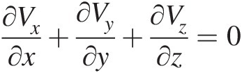 (2.130)

2.2.9.2 Inertial Reference Frame: Cylindrical Coordinates
In this coordinate system, the velocity V→ (also called absolute velocity) has components Vr, Vθ,Vr,Vθ, and VxVx in r, θ,r,θ, and xx(axial) coordinate directions respectively, as shown in Figure 2.13a. Equation 2.215 in each coordinate direction and the continuity equation are written as follows:
rr-coordinate direction:
 (2.131)
θθ-coordinate direction:
 (2.132)
xx-coordinate direction:
 (2.133)
Continuity equation:
∂Vr∂r+Vrr+1r∂Vθ∂θ+∂Vx∂x=0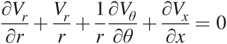 (2.134)


Figure 2.13 (a) Inertial cylindrical coordinate system and (b) rotating (noninertial) cylindrical coordinate system.
Note that the last term −Vθ2/r within brackets on the left-hand side of Equation 2.131 is the centripetal acceleration (negative of the centrifugal acceleration), which results from the flow tangential velocity. For Vr < < Vθ, Vx < < Vθ, Fr = 0,Vr<<Vθ,Vx<<Vθ,Fr=0, and away from the viscosity dominated region, Equation 2.131 reduces to ∂Ps/∂r=ρVθ2/r
 , which is known as the radial equilibrium equation for a rotating flow.
2.2.9.3 Noninertial Reference Frame: Cylindrical Coordinates with Constant Rotation
Let us now consider a cylindrical coordinate system with its coordinate axes rotating with constant Ω→ along an arbitrary axis of rotation, as shown in Figure 2.13b for constant rotation around the xx axis. In this coordinate system, which is noninertial, the flow velocity W→
 (also called relative velocity) has components Wr, Wθ,Wr,Wθ, and WxWx in r, θ,r,θ, and xx(axial) coordinate directions, respectively. The relative velocity W→
 is related to the absolute velocity V→
 by the following equation:
 (2.135)
where r→ is the position vector in the rotating reference frame.
Centrifugal and Coriolis forces. Using Equation 2.135, the N–S equations (Equation 2.125) in absolute velocity can be easily converted (see Greitzer, Tan, and Graf (2004) for details) into the corresponding equations in relative velocity of the rotating coordinate system
 (2.136)
Transferring ρΩ→×Ω→×r→ and 2ρΩ→×W→
 to the right-hand side of Equation 2.136, we obtain
 (2.137)
Note that the left-hand side of Equation 2.137, representing the substantial derivative of the relative velocity W→ , is identical in form to the left-hand side of Equation 2.125, which uses the absolute velocity V→
 . Further note that the pressure forces, viscous forces, and F→
 on the right-hand side of Equation 2.137 also take the same form as in Equation 2.125.
On the right-hand side of Equation 2.137, ρΩ→×(Ω→×r→) and 2ρΩ→×W→
 are the centrifugal force and Coriolis force per unit volume, respectively. Because these forces have no resemblance to the forces that appear in this equation, they are sometimes referred to as the “fictitious forces” for an observer in the inertial reference frame. These forces, however, are real for an observer in the rotating (noninertial) reference frame. They simply arise from the kinematics of going from rotating reference frame, which is noninertial, to an inertial reference frame in which the Newton’s laws of motion are valid. Note that the vector that results from ρΩ→×(Ω→×r→)
 is co-linear with r→
 and points toward the origin (centripetal). Any relative velocity component in the direction of Ω→
 will have no contribution to the Coriolis force (2ρΩ→×W→
 ). Only the relative velocities in a plane normal to the direction of Ω→
 will contribute to this force.
Let us now see how we can express the centrifugal force ρΩ→×(Ω→×r→) as the gradient of a scalar quantity, just as the conservative gravitation force can be expressed as the gradient of a potential function. Without loss of generality, let the xx axis in our rotating coordinate system coincide with the rotational velocity vector Ω→
 . Then the radius of rotation will be measured off this axis, and (Ω→×r→)
 can be written as (Ω→×rêr)
 , where êr
 is the unit vector in the radial direction, because the component of the displacement vector r→
 along the direction of Ω→
 will have no contribution to the cross product. Thus, we obtain ρΩ→×(Ω→×r→)=ρΩ→×(Ω→×rêr)
 . Using the vector identity A→×(B→×C⇀)=B→(A→•C⇀)−C⇀(A→•B→)
 , we can write ρΩ→×(Ω→×r→)=ρΩ→×(Ω→×rêr)=−ρrΩ2êr
 , which can be further expressed as ∇(−ρ r2Ω2/2)∇−ρr2Ω2/2. Using this result in Equation 2.137 and defining a reduced static pressure P˜s=Ps−ρr2Ω2/2
 , we can alternatively write this equation as
 (2.138)
which reveals that the net effect of the centrifugal force as a result of rotation of the coordinate system is to alter the static pressure field to the extent needed to balance this centrifugal force.
A cylindrical coordinate system rotating with constant ΩΩ about the xx axis, which could be thought of as the gas turbine axis of rotation, is shown in Figure 2.13b. For this case, Equation 2.137 in each coordinate direction and the continuity equation can be written as follows:
rr-coordinate direction:
 (2.139)
θθ-coordinate direction:
 (2.140)
xx-coordinate direction:
 (2.141)
Continuity equation:
 (2.142)
In the radial direction, according to Equation 2.139, we have two centrifugal force terms ρWθ2/r and ρΩ2rρΩ2r, the first results from the relative tangential velocity WθWθ of the flow, and the second from the fact that the coordinate system is rotating with constant ΩΩ. Note that the Coriolis force has two components. The component 2ρΩ Wθ2ρΩWθ is in the radial direction and (−2ρΩ Wr−2ρΩWr) in the tangential direction (Equation 2.139).
The centrifugal and Coriolis forces are real forces in a rotating noninertial reference frame. We often experience centrifugal forces while driving on a curve or when a car skids on an icy road with a sharp turn. If you are standing on a counterclockwise rotating platform, such as a merry-go-round in a theme park, you will experience a centrifugal force trying to push you radially outward. If the platform is slippery or icy, you will soon slip to the outer edge of the platform, but not exactly along the radial direction from where you started. As you are slipping radially outward, you will gradually turn to your right as a result of the Coriolis force.
Consider a steady, two-dimensional, incompressible, inviscid flow from a source located at the origin (r = 0r=0). For an observer in an inertial reference frame, the flow will have radial streamlines emanating from the origin with the absolute radial velocity VrVr, decaying inversely with radius to satisfy continuity. The static pressure gradient ∂Ps/∂r∂Ps/∂r in this flow will equal (−ρVr∂Vr/∂r)−ρVr∂Vr/∂r. This pressure gradient is independent of the reference frame. The kinematics of this source flow will appear different to an observer in a reference frame rotating counterclockwise at an angular velocity ΩΩ. This observer will see the flow having two velocities in the plane, one radial Wr = VrWr=Vr and the other tangential Wθ = − rΩWθ=−rΩ, spiraling away from the origin at lower radii and assuming circular streamlines for Vr < < WθVr<<Wθ. Because the pressure gradient at each radial location also equals (−ρWr∂Wr/∂r)−ρWr∂Wr/∂r, we find that the additional centrifugal force term due to the tangential velocity (WθWθ), ρWθ2/r=ρrΩ2 , together with the centrifugal force ρrΩ2ρrΩ2 as a result of coordinate system rotation cancels the Coriolis force (2ρΩWθ = − 2ρrΩ22ρΩWθ=−2ρrΩ2).
The existence of the Coriolis and centripetal accelerations as a result of coordinate system rotation is easily demonstrated for a vortex flow with circular streamlines and circular isobars. For a streamline of radius rr with velocity VθVθ in this flow, the centripetal acceleration Vθ2/r in the inertial reference frame is driven by the static pressure gradient ∂Ps/∂r∂Ps/∂r; recall the local equilibrium equation ∂Ps/∂r=ρVθ2/r
 . Substituting Vθ = Wθ + rΩVθ=Wθ+rΩ for the rotating reference frame, we obtain Vθ2/r=Wθ2/r+2ΩWθ+rΩ2
 , which shows that the centripetal acceleration Wθ2/r
 in the rotating reference frame is not sufficient to yield the required static pressure gradient, which is independent of the reference frame. The Coriolis acceleration 2ΩWθ2ΩWθ and the centripetal acceleration rΩ2rΩ2 as a result of coordinate system rotation are needed to make up for the difference.
To develop further insight into the centrifugal and Coriolis forces, let us consider a frictionless water sprinkler shown in Figure 2.14. Only one sprinkler arm is shown flowing, the other is blanked off. Each arm is made of a straight pipe in the radial direction and a curved pipe in the form of a circular arc, having the radius of curvature equal to that of the circle traversed by the sprinkler. For the sprinkler, the maximum angular velocity is given by Ω = Wθ/RΩ=Wθ/R, where WθWθ is the constant relative tangential velocity in the curved pipe. The radial pipe has constant relative radial flow velocity WrWr and has no tangential and axial velocities.

Figure 2.14 A sprinkler system featuring centrifugal and Coriolis forces.
In the blanked-off arm of the sprinkler, water is in a rigid-body rotation. Because all relative velocity components are zero in this arm, there are no Coriolis forces. However, the centrifugal force in this arm corresponds to ρ Ω2rρΩ2r, increasing linearly with radius. As a result, we have uniform static pressure at each section of the straight pipe, but radially increasing static pressure distribution in each section of the curved pipe, as shown in Figure 2.14 for sections A and B.
In the rotating sprinkler arm that is flowing, the straight pipe features a radial velocity WrWr and will generate a uniform Coriolis force (−2ρΩWr−2ρΩWr) in the negative tangential direction, causing a static pressure gradient in the direction shown for section C in Figure 2.14. The flow features in the curved pipe with flow are quite interesting. In this rotating pipe, we have no radial static pressure gradient at any section, as shown for section D in Figure 2.14. How do we explain this apparently nonintuitive flow behavior? The answer lies in finding the centrifugal and Coriolis forces in this pipe. Because the absolute flow velocity in this pipe is zero (Vθ = RΩ − Wθ = 0Vθ=RΩ−Wθ=0), the centrifugal force ρVθ2/R=0 , resulting in a radially uniform static pressure distribution. Now, let us look at the centrifugal and Coriolis forces in the rotating reference frame attached to the sprinkler. The centrifugal force from WθWθ equals ρWθ2/R
 and that from ΩΩ equals ρΩ2RρΩ2R. Because Ω = Wθ/RΩ=Wθ/R, both these forces are equal, giving 2ρΩ2R2ρΩ2R as the total centrifugal force. The Coriolis force in this curve pipe can be computed as 2ρΩ(−Wθ) = − 2ρΩ2R2ρΩ−Wθ=−2ρΩ2R, which is opposite and equal to the centrifugal force, yielding a net zero force, which we concluded from using the absolute velocity (inertial reference frame).
2.2.9.4 Rotating Couette Flow
In this section, we demonstrate a procedure to obtain exact solutions of the Navier-Stokes equations governing a steady incompressible laminar flow between concentric cylinders of radii R1R1 and R2R2, as shown in Figure 2.15. Among other applications, like CFD validation, the solutions offer a basis for measuring fluid viscosity by a device. In this case, the inner cylinder is rotating at a constant angular velocity Ω1Ω1, and the outer cylinder with Ω2Ω2, with no imposed pressure gradient and zero flow in the axial direction (Vx = 0Vx=0).

Figure 2.15 Couette flow between two concentric, rotating cylinders.
The solutions developed here are based on the following assumptions for the flow being: (i) axisymmetric (∂/∂θ = 0∂/∂θ=0), (ii) fully developed (∂/∂x = 0∂/∂x=0), and (iii) with zero body force as a result of gravity.
Continuity equation in cylindrical coordinates. The continuity equation, Equation 2.134, in the inertial cylindrical polar coordinates is expressed as


Using Vx = ∂Vθ/∂θ = 0Vx=∂Vθ/∂θ=0 from the assumptions, this equation reduces to

whose integration yields rVr = CrVr=C in rr direction, where CC is the integration constant. Because Vr = 0Vr=0 at the inner cylinder wall at r = R1r=R1, it must be zero everywhere in the flow, giving C = 0C=0.
Reduced Navier-Stokes Equations in cylindrical coordinates. With Vx = 0Vx=0, the xx-momentum equation, Equation 2.133, is identically satisfied. Under the assumptions made in this problem and Vr = 0Vr=0 from the continuity equation, the rr-momentum equation, Equation 2.131, reduces to
 (2.143)
which governs the radial distribution of the static pressure between two cylinders.
The θθ-momentum equation, Equation 2.132, reduces to

which can be alternatively written as
 (2.144)
Equation 2.144 is a homogeneous second-order ordinary differential equation and requires two boundary conditions for a unique solution. These two boundary conditions in this case correspond to no-slip condition at the walls of the inner and outer cylinders, namely, Vθ = R1Ω1Vθ=R1Ω1@r = R1r=R1 and Vθ = R2Ω2Vθ=R2Ω2@r = R2r=R2.
Tangential velocity distribution. Integrating Equation 2.144 once, we obtain


Integrating this equation once more yields

where C1=C˜/2 . Thus, the general solution for the distribution of VθVθ between the cylinders is given by
where C1C1 and C2C2 are the integration constants, which are to be determined from the boundary conditions at the inner and outer cylinders, yielding the following two equation:
Solving the aforementioned two simultaneous algebraic equations yields:
 (2.146)
and
 (2.147)
Substituting Equations 2.146 and 2.147 into Equation 2.145, we finally obtain
 (2.148)
Static pressure distribution. Substituting for VθVθ from Equation 2.145 into Equation 2.143, we obtain

which upon integration and substitution for C1C1 and C2C2 from Equations 2.146 and 2.147, respectively, finally yields
 (2.149)
where Ps1Ps1 is the static pressure at the surface of the inner cylinder.
Torques on inner and outer cylinders. The torque on each cylinder, per unit length in the axial direction, can be computed as the product of the wall shear stress, cylinder circumference, and radius. Knowing the distribution of velocity VθVθ from Equation 2.148, we can evaluate the tangential shear stress distribution in the flow between the two cylinders by the equation

Substituting for VθVθ yields
 (2.150)
For r = R1r=R1, Equation 2.150 yields the torque on the inner cylinder

Similarly, for r = R2r=R2, Equation 2.150 yields the torque on the outer cylinder

Note that the torques Γ1Γ1 and Γ2Γ2 on the two cylinders are equal and opposite, implying zero net torque acting on the fluid; as a result, its angular momentum remains constant.
2.2.9.5 Taylor-Proudman Theorem
Taylor-Proudman theorem embodies the behavior of a steady, incompressible, laminar flow that is dominated by rotation (Coriolis forces). To understand this theorem, let us consider the Navier-Stokes equation, Equation 2.138. When we use the velocity scale WrefWref and length scale LrefLref to nondimensionalize this equation, two dimensionless numbers emerge. The first is called the Rossby number Ro = Wref/ΩLrefRo=Wref/ΩLref and the second, the Ekman number Ek=μ/ρΩLref2 . While the Rossby number is a measure of the inertia force associated with the relative velocity in comparison to the Coriolis forces, the Ekman number is the ratio of viscous forces to Coriolis forces. For a steady incompressible flow outside a wall boundary layer and with Ro < < 1Ro<<1 and Ek < < 1Ek<<1, that is, the Coriolis forces dominate over the inertia and viscous forces, Equation 2.138 reduces to
 (2.151)
The flows that are governed by Equation 2.151 are known as geostrophic flows in which the modified (by including the potential function associated with the centrifugal forces as a result of the rotation of the coordinate axes) static pressure gradients are balanced by the Coriolis forces.
Taking the curl of both sides of Equation 2.151 and noting that the curl of the gradient of a scalar function is identically zero, we obtain
 (2.152)
Using the vector identity ∇×(A→×B→)=(B→•∇)A→−B→(∇•A→)−(A→•∇)B→+A→(∇•B→) and invoking the continuity (∇•W→=0
 ) and the fact that Ω→
 is constant, we finally obtain from Equation 2.152
 (2.153)
Assuming the direction of Ω→ as the axis of rotation along the xx direction, Equation 2.153 yields ∂W→/∂x=0
 , which indicates that all three components of the relative velocity do not change in the direction parallel to the axis of rotation – the statement of the Taylor-Proudman theorem. In a flow system with solid boundaries perpendicular to the axis of rotation, we have Wx = 0Wx=0 at some specified value of xx. The Taylor-Proudman theorem implies that this flow system will remain entirely two-dimensional in planes perpendicular to the axis of rotation.
Taylor columns. Taylor columns are a unique and interesting manifestation of the Taylor-Proudman theorem. These columns occur when there is relative motion between an obstacle and fluid in a rotating system dominated by rotation. To illustrate a Taylor column, let us consider a rotating cylinder filled with liquid. We have a short cylinder attached to the bottom surface of the cylinder. If you rotate this system at some angular velocity ΩΩ, eventually the liquid will attain solid-body rotation with all the solid surfaces. Now, if we reduce the cylinder angular velocity slightly, the liquid will continue to rotate at the old angular velocity and develop a relative velocity (Ωliquid>ΩcylinderΩliquid>Ωcylinder) such that the short cylinder at the bottom of the rotating cylinder is rendered into cross-flow with the surrounding fluid, as shown in Figure 2.16.

Figure 2.16 Taylor column.
In the flow system shown in Figure 2.16, as a result of strong rotation, there is no flow on the top of the short cylinder. According to the Taylor-Proudman theorem, the velocity components will not change in the direction of the axis of rotation, the xx direction in this case. As a result, a solid column of liquid develops on the top of the short cylinder, as if the cylinder is extended up to the free surface of the liquid in the rotating cylinder. In planes perpendicular to the xx axis, we have identical two-dimensional velocity distributions, as shown in the figure.
2.2.9.6 Ekman Boundary Layers
Rotor surfaces associated with rotor disks and rotor cavities abound in gas turbines. Boundary layers formed on these surfaces are generally known as Ekman layers. These layers feature some unique characteristics not found in a typical boundary layer such as the one developed on a flat plate under zero pressure gradient where wall shear stress reduces momentum in the flow direction, resulting in a continuously (growing) thickening boundary layer. In contrast, the Ekman layer does not entrain fluid from the region outside the boundary layer and consequently maintains a constant thickness. For low Rossby numbers, where the Ekman boundary layer is sandwiched between the geostrophic flow and the rotating wall, we obtain a set of linear boundary layer equations with closed-form analytical solutions for the distributions of velocities in the boundary layer. These solutions, systematically developed here, provide further insight into an Ekman layer.
Let us consider a rotating disk whose axis of rotation is along the xx-axis. For an axisymmetric (∂/∂θ = 0∂/∂θ=0), steady, incompressible, laminar flow with constant viscosity, no body forces, and Ro < < 1Ro<<1, the Navier-Stokes equations (Equations 2.139, 2.140, and 2.141) reduce to:
rr-momentum equation:
 (2.154)
θθ-momentum equation:
 (2.155)
xx-momentum equation:
 (2.156)
where we have used the reduced pressure given by P˜s=Ps−ρr2Ω2/2 . The continuity equation (Equation 2.142) also simplifies to
 (2.157)
The flow field outside the disk boundary layer (Ekman layer) is assumed geostrophic (Ro < < 1Ro<<1 and Ek < < 1Ek<<1) with relative velocities Wr∞, Wθ∞,Wr∞,Wθ∞, and Wx∞Wx∞. From the Taylor-Proudman theorem, discussed in Section 2.2.9.5, we know that these velocities do not vary along the xx direction. From Equation 2.155, without the viscous terms on the right-hand side, we obtain Wr∞ = 0Wr∞=0 which should prevail at the outer edge of the Ekman layer. Substituting Wr∞ = 0Wr∞=0 in Equation 2.157 simply yields ∂Wx/∂x = 0∂Wx/∂x=0, which is also obtained from the Taylor-Proudman theorem.
Under the assumption ∂(rWr)/∂r = 0∂rWr/∂r=0 within the Ekman layer, Equation 2.157 yields ∂Wx/∂x = 0∂Wx/∂x=0, that is, WxWx is constant across the boundary layer. Because, as a result of no slip condition, Wx = 0Wx=0 at the wall, we obtain Wx = 0Wx=0 everywhere in the boundary layer, which implies that the Ekman boundary layer is nonentraining. We further conclude that Wx∞ = 0Wx∞=0. Substituting Wx = 0Wx=0 in Equation 2.156, we obtain ∂P˜s/∂x=0 , that is, the reduced static pressure also does not vary along the rotation axis, both in the Ekman layer and the outside geostrophic flow.
In the geostrophic flow region, Equation 2.154 yields
 (2.158)
Combining Equations 2.154 and 2.158 and noting that rWr = 0rWr=0, we obtain the following rr-momentum equation in the Ekman boundary layer
 (2.159)
where ν = μ/ρν=μ/ρ is the kinematic viscosity.
Because

in Equation 2.155, we can finally write the θθ-momentum equation in the Ekman boundary layer as
 (2.160)
Equations 2.159 and 2.160 indicate that the Coriolis forces are in balance with the shear forces in an Ekman boundary layer. The relevant boundary conditions to solve these coupled second-order differential equations are as follows:
To facilitate the solution of the system of Ekman boundary layer equations and boundary conditions, let us define the following dimensionless variables:

Using these variables, Equations 2.159 and 2.160 can be re-written as
 (2.163)
and
 (2.164)
Let us now define a complex velocity Z=W˜θ+iW˜r . Multiplying Equation 2.164 by ii and adding it to Equation 2.163, we obtain the second-order differential equation
 (2.165)
with the boundary conditions, which correspond to Equations 2.161 and 2.162, given by
and
We can write the general solution of Equation 2.165 as
where the coefficients AA and BB need to be determined from the boundary conditions. From the second boundary condition (Equation 2.167), we obtain B = 0B=0, and the first boundary condition (Equation 2.166) yields A = − 1A=−1. Thus, the closed-form analytical solution of Equation 2.165 finally becomes
Equating the real and imaginary parts on both sides of Equation 2.169, we finally obtain
 (2.170)
and
 (2.171)
It is interesting to note from Equation 2.170 that for Wθ∞>0Wθ∞>0, which means that the fluid in the geostrophic region is rotating faster than the wall, the flow in the Ekman boundary layer is radially inward. Conversely, for Wθ∞ < 0Wθ∞<0, we will have radially outward flow in the Ekman layer.
Distributions of radial and tangential velocities, based on Equations 2.170 and 2.171, are depicted in Figure 2.17 for the case with Wθ∞ < 0Wθ∞<0. The undershoot of the radial velocity for π < ζ < 2ππ<ζ<2π, representing a slight flow reversal in the Ekman layer, and the overshoot of the tangential velocity for π/2 < ζ < 3π/2π/2<ζ<3π/2 are interesting features not found in boundary layers in nonrotating flow systems. In Figure 2.17, the plot of θ˜ , which is the angle the resultant velocity vector in the Ekman boundary layer makes with the tangential velocity, shows that it varies from zero at the edge of the boundary layer to 45°45° near the wall, exhibiting a spiraling fluid motion, which is known as Ekman spiral.

Figure 2.17 Velocity distributions in an Ekman boundary layer.
2.3 Internal Flow
Many of the general concepts of fluid mechanics are discussed in Section 2.2. Some of the special concepts, which are founded in the conservation laws of mass, momentum, energy, and entropy and widely used in gas turbine design engineering, are presented in this section.
These concepts include isentropic and nonisentropic vortices, windage, and the relation between the loss coefficient and discharge coefficient for both incompressible and compressible flows. This section also includes the quantitative evaluation of static and total pressures and temperatures in a nonisentropic generalized vortex, which is an important feature of gas turbine internal flow systems.
2.3.1 Isentropic and Nonisentropic Vortices: Pressure and Temperature Changes
2.3.1.1 Isentropic Free Vortex
A free vortex is characterized by constant angular momentum, and it must be free from any applied torque. As such it is seldom found in a gas turbine internal flow system, but the tendency toward a free vortex behavior exits in radial inflows in a rotor cavity. Often, the flowpath designs of turbine blades are based on a free vortex assumption. It is, however, instructive to model a free vortex and understand how pressure and temperature change in this vortex flow.
Like the Euler’s turbomachinery equation, discussed in Section 2.2.7, we will formulate here an isentropic free vortex in the inertial reference frame. To see how such a formulation is simpler than the alternative formulation in the rotor reference frame, let us examine the radial equilibrium equation in both reference frames. Converting Equation 2.143 in the rotor reference frame, we obtain
 (2.172)
Compared to one term, representing the centrifugal force per unit volume on the right-hand side of Equation 2.143, the right-hand side of Equation 2.172 consists of three terms: (1) the centrifugal force as a result of the relative tangential velocity, (2) the Coriolis force, and (3) the centrifugal force as a result of rotation of the rotor reference frame.
It is customary to express the fluid absolute tangential velocity as a fraction of the local tangential velocity of the rotor. Thus, we define the local swirl factor of a vortex flow as
 (2.173)
For a free vortex, we can express the swirl factor and tangential velocity, shown in Figure 2.18, by the following equations:
 (2.174)
and
 (2.175)
where C1C1 is a constant related to the vortex strength.

Figure 2.18 (a) Radial variation of swirl factor in free and forced vortices and (b) Radial variation of tangential velocity in free and forced vortices.
Static pressure and static temperature variations in an isentropic free vortex. Using the equation of state to replace ρρ in the radial equilibrium equation, we obtain
 (2.176)
For an isentropic (ds = 0ds=0) vortex flow, substituting

from Equation 2.15 into Equation 2.176 yields
 (2.177)
Substituting for VθVθ from Equation 2.174 yields

which upon integration between states 1 and 2 further yields
 (2.178)
and can be easily expressed in the form
 (2.179)
where
 (2.180)
Using the relation between pressure ratio and temperature ratio in an isentropic flow, we can write
 (2.181)
Total pressure and total temperature variations in an isentropic free vortex. Knowing the static temperature and velocity components at any point of a free vortex, we can compute the total temperature by the equation

If the axial and radial velocities do not change between two points, the aforementioned equation yields
 (2.182)
which shows that the change in total temperature between two points consists of two parts: the change in static temperature and the change in dynamic temperature.
Using Equation 2.174, Equation 2.182 becomes

which upon substitution from Equation 2.178 reduces to
Equation 2.183 reveals an interesting, but expected, result that there is no change in total temperature in an isentropic free vortex. In this case, the change in static temperature is opposite and equal to the change in the dynamic temperature resulting from the change in the tangential velocity. Thus, for an isentropic free vortex we obtain Tt2/Tt1 = 1Tt2/Tt1=1 and Pt2/Pt1 = 1Pt2/Pt1=1.
2.3.1.2 Isentropic Forced Vortex
Like every particle in a solid-body rotation, the fluid in a forced vortex rotates at a constant angular velocity. Thus, unlike a free vortex, the tangential velocity in a forced vortex increases linearly with radius. Figure 2.18 shows the radial variations of the tangential velocity and swirl factor in a forced vortex. The flow in a rotating duct behaves like a forced vortex. With the constant swirl factor (Sf = C2Sf=C2) characterizing a forced vortex, the linear variation of the tangential velocity with radius can be expressed as
where C2C2 is a constant representing the vortex strength as a fraction of the rotor angular velocity ΩΩ.
Static pressure and static temperature variations in an isentropic forced vortex. Equation 2.177 is valid for all isentropic vortex flows. For a forced vortex, we use Equation 2.184 to replace VθVθ in this equation, giving
 (2.185)
Integration of Equation 2.185 between states 1 and 2 yields
 (2.186)
which shows that the change in static temperature between any two points of an isentropic forced vortex equals the change in the dynamic temperature at these points. Upon further rearrangement, Equation 2.186 becomes
 (2.187)
where
 (2.188)
Using the relation between pressure ratio and temperature ratio in an isentropic flow, we finally obtain
 (2.189)
Comparing Equations 2.179 and 2.187 for static temperature change in a free vortex and a forced vortex, respectively, we can write
 (2.190)
Equation 2.190 indicates that, for both radially outward (r2>r1r2>r1) and radially inward (r1>r2r1>r2) flows with identical conditions at r1r1 (inlet), the static temperature at r2r2 (outlet) for a forced vortex is always higher than that for a free vortex. Similarly, comparing Equations 2.181 and 2.189, we conclude that, with the identical conditions at r1r1 (inlet), the static pressure at r2r2 (outlet) for a forced vortex is always higher than that for a free vortex. These observations have important repercussions in the design of internal flow systems of gas turbines.
Total pressure and total temperature variations in an isentropic forced vortex. Equations 2.182 and 2.184 yield
 (2.191)
on the right-hand side of which the first expression within the parentheses represents the change in static temperature and the remaining terms represent the change in dynamic temperature based on the tangential velocity.
Using Equation 2.186, we can express Equation 2.191 as
which shows that, between any two points, the change in total temperature in an isentropic forced vortex equals twice the change in its static temperature, and can be alternatively expressed as
 (2.193)
Using the relation between the ratio of total pressures and ratio of total temperatures between any two points in an isentropic flow, we obtain
 (2.194)
2.3.1.3 Isothermal Forced Vortex
An accurate prediction of the static pressure distribution on a rotor disk forming a rotor-rotor or rotor-stator cavity of a gas turbine is critical to the evaluation axial rotor thrust. The current design practice by and large is based on the static pressure distribution in a series of isentropic force vortices, neglecting the effect of temperature change as a result of heat transfer on this distribution. In this section, we will examine such an effect by finding the analytical solution of static pressure distribution in an isothermal forced vortex and comparing it to the one for the isentropic case derived in the foregoing section.
In an isothermal forced vortex, the static temperature is assumed to remain constant between any two points. This implies cooling of a radially outward flowing forced vortex and heating of a radially inward flowing forced vortex, which are otherwise isentropic. Using Equations 2.176 and 2.184 we can write
 (2.195)
which can be integrated between two points to yield
 (2.196)
Variations of static pressure in a forced vortex under isentropic and isothermal flow conditions, based on Equations 2.189 and 2.196, are shown in Figure 2.19 for κ = 1.4κ=1.4 and Mθ1 = 0.5Mθ1=0.5. Beyond a small change in radius, radial variation of static pressure in an isothermal forced vortex is higher than that in an isentropic forced vortex. The comparison shown in this figure indicates that, for an accurate prediction of static pressure in a forced vortex, we must account for temperature variation as a result of heat transfer, as discussed in Section 2.3.1.4 for a nonisentropic generalized vortex.

Figure 2.19 Comparison of static pressure variations in isentropic and isothermal forced vortices.
2.3.1.4 Nonisentropic Generalized Vortex
A nonisentropic generalized vortex is characterized by an arbitrary radial distribution of swirl factor Sf = f1(r)Sf=f1r and total temperature Tt = f2(r)Tt=f2r, which results from both heat transfer and rotational work transfer. The functions f1(r)f1r and f2(r)f2r are piecewise polynomial functions between radii r1r1 and r2r2. The static pressure variation in this vortex is governed by Equation 2.176, which can be expressed in terms of rotational Mach number as
 (2.197)
where Mθ=Vθ/κRTs in which Vθ = SfΩ r = f1Ω rVθ=SfΩr=f1Ωr and Ts=Tt−Vθ2/(2cp)=f2−f12Ω2r2/(2cp)
 .
.
Integrating Equation 2.197 between radii r1r1 and r2r2, we can write
 (2.198)
where GG is computed by numerically integrating ∫r1r2Mθ2rdr , for example, using the Simpson’s one-third rule. Thus, we finally obtain the following equation to compute static pressure distribution in a nonisentropic generalized vortex:
2.3.2 Windage versus Vortex Temperature Change
In internal flow systems of a gas turbine, the fluid total temperature will change as a result of heat transfer from both rotor and stator surfaces and work transfer only from the rotor surfaces. As a result of the fact that the stator wall is not moving relative to the fluid (no-slip boundary condition as a result of nonzero fluid viscosity), the wall shear stress cannot participate in any work transfer between the fluid and the wall. For example, the total temperature of the fluid flowing through an adiabatic stationary duct with friction will remain constant in the duct. Windage is, therefore, defined as rotor power input into the surrounding fluid. It should not be confused with viscous dissipation, which results from viscosity-driven transfer of external flow energy into the internal energy with no change in fluid total temperature under adiabatic conditions.
Figure 2.20 shows a typical rotor-stator cavity where the windage is generated by the rotor surface. For the windage analysis between sections 1 and 2, let us consider the control volume ABCD. The angular momentum balance over this control volume yields
 (2.200)
where ΓBC, rotorΓBC,rotor and ΓAD, statorΓAD,stator are, respectively, the rotor torque and the stator torque within the control volume, determined using empirical equations. Windage power is then computed as
 (2.201)
Figure 2.20 A typical windage situation in a gas turbine rotor-stator cavity.
Combining Equations 2.200 and 2.201 yields
 (2.202)
Equation 2.202 is often misinterpreted to imply that the first term on its right-hand indicates the work done by the stator, which cannot do any work. To avoid such a nonphysical interpretation, one should use Equations 2.200 and 2.201 separately, the first originating from the angular momentum equation and the second from the energy equation.
The change in total temperature as a result of windage power can be obtained from Equation 2.201 as
 (2.203)
Note that the process of windage generation is nonisentropic. Any design practice to calculate forced vortex temperature change using Equation 2.193 in the control volume and adding to the temperature change computed from Equation 2.203 will be in violation of the energy equation and must be avoided. To further illustrate this flawed design practice, if it exists, let us consider an all-stator cavity shown in Figure 2.21a. Because there is no rotor surface, although the swirl factor will decrease (Sf2 < Sf1Sf2<Sf1) from inlet to outlet as a result of the torque from the stator walls, the total temperature will remain constant under adiabatic conditions. In the case of rotor-stator cavity shown in Figure 2.21b, one must use Equation 2.203 to compute the change in total temperature from inlet to outlet.

Figure 2.21 Total temperature change in: (a) all-stator cavity, (b) rotor-stator cavity, and (c) rotating pipe.
For the flow through a rotating pipe, shown in Figure 2.21c, where the constant swirl factor corresponds to solid-body rotation (Sf = 1Sf=1), the change in total temperature from inlet to outlet can be established as isentropic forced vortex temperature rise (Equation 2.193), which also equals the windage temperature rise based on the work transfer computed using the Euler’s turbomachinery equation. Readers are encouraged to verify on their own that ΔTtwindage = ΔTtforced vortexΔTtwindage=ΔTtforced vortex in this case.
2.3.3 Loss Coefficient versus Discharge Coefficient
In incompressible internal flows, it is customary to simulate minor losses using the incompressible loss coefficient KK, which is defined as
 (2.204)
In Equation 2.204, the dynamic pressure used as the denominator of the right-hand side term corresponds to either inlet or outlet, whichever is higher. Values of KK for various flow elements are reported for example in Idelchik (2005). No such comprehensive empirical data for minor losses for compressible flows yet exist. A common engineering practice, which may not be physics-based, is to extend the use of Equation 2.204 for compressible flows by replacing the denominator with (Ptinlet − Psinlet)Ptinlet−Psinlet or (Ptoutlett − Psoutlet)Ptoutlett−Psoutlet, whichever is higher. As the Mach number increases, so does the dynamic pressure over the corresponding incompressible value.
Another approach to simulate minor losses in both incompressible and compressible flows is through the discharge coefficient CdCd, which is simply defined by the equation
 (2.205)
where the ideal mass flow rate ṁideal through the element is computed under no loss in total pressure. Note that the discharge coefficient CdCd is usually determined empirically.
Relation between KK and CdCd for an incompressible flow. Let us derive a relationship between KK and CdCd for an incompressible flow through a sudden pipe contraction shown in Figure 2.22. According to Equation 2.204, we can write in this case


Figure 2.22 Relation between loss coefficient and discharge coefficient of a sudden pipe contraction.
Using this, we can write the mass flow rate through a sudden contraction pipe flow element as
 (2.206)
To calculate the ideal mass flow rate through the flow element, we assume that the inlet total pressure remains constant. Accordingly, we can write

which yields
 (2.207)
Thus, using Equation 2.205, we can express the actual mass flow rate as
 (2.208)
Equating mass flow rates computed by Equations 206 and 208, we finally obtain
 (2.209)
which is identical to the equation obtained by Sultanian (2015) for an orifice with incompressible flow. It is, however, important to note that the relation between KK and CdCd given by Equation 2.209 is not a universal one. For example, using the foregoing procedure for a sudden expansion pipe flow will yield a relationship between KK and CdCd with dependence on the expansion area ratio (see Problem 2.14).
Relation between KK and CdCd for a compressible flow. Let us now derive a relationship between KK and CdCd for a compressible flow through the sudden pipe contraction shown in Figure 2.22 and compare it with Equation 2.209. In this case, we define the compressible loss coefficient by the equation
 (2.210)
which yields
 (2.211)
and
 (2.212)
Using Equation 2.103, we can compute mass flow rate through the sudden contraction flow element as
 (2.213)
where F̂ft is the dimensionless total-pressure mass flow function given by
 (2.214)
Where the Mach number M2M2 is to be determined by the equation
 (2.215)
which uses outlet pressure ratio Pt2/Ps2Pt2/Ps2 from Equation 2.212.
Again for computing ideal mass flow rate through the flow element, we assume no loss in total pressure under adiabatic conditions, implying Pt2 = Pt1Pt2=Pt1 and Tt2 = Tt1Tt2=Tt1, and yielding
 (2.216)
where
 (2.217)
where
 (2.218)
Expressing the actual mass flow rate in terms of the discharge coefficient as
 (2.219)
and equating it with the mass flow rate computed from Equations 2.213, we obtain

which with the substitution of Pt2Pt2 from Equation 2.211 becomes
 (2.220)
Thus, for a compressible flow through a sudden pipe contraction, Equation 2.220 relates KK and CdCd. Unlike for the case of incompressible flow (Equation 209), Equation 2.220 for the compressible flow shows that the relationship between KK and CdCd also depends on the overall pressure ratio Pt1/Ps2Pt1/Ps2.
Figure 2.23 compares the variation of discharge coefficient with loss coefficient for both incompressible flow (Equation 209) and compressible flow (Equation 2.220) with κ = 1.4κ=1.4 and Pt1/Ps2 = 1.8Pt1/Ps2=1.8. For Pt1/Ps2 < 1.1Pt1/Ps2<1.1, when a compressible flow can be treated as an incompressible flow with constant density, two curves are virtually identical for all values of KK. A mathematical reduction of Equation 2.220 to Equation 2.209 for low values of Pt1/Ps2Pt1/Ps2 is not evident.

Figure 2.23 Variation of discharge coefficient with loss coefficient in a sudden pipe contraction for both incompressible and compressible flows.
2.4 Heat Transfer
In gas turbine internal flow systems, both heat transfer and work transfer, separately or simultaneously, are responsible for any change the fluid temperature. We define heat transfer between the fluid and solid structure, or within the solid itself, as energy transfer by virtue of a temperature difference. Work transfer into the fluid will only occur if the solid wall in contact is rotating. There can be no work transfer when the fluid flows over any static structure. It is important to note that heat transfer always occurs from high to low temperature, and never the other way around. A fluid flow, however, can occur against an increasing static pressure, as in a diffuser, as a result of the associated inertia. There is no such thing as thermal inertia associated with heat transfer, and the direction of decreasing temperature uniquely determines the direction of heat transfer.
Now, consider a turbine airfoil with internal cooling. Often a thermal barrier coating (TBC) with very low thermal conductivity is used on the airfoil surface exposed to hot gases to reduce heat transfer to the internal cooling flow. To improve turbine efficiency, one may be tempted to a heat transfer design solution that eliminates the internal cooling flow by increasing TBC thickness or by using a TBC with much lower thermal conductivity. Because the temperature difference exists between the hot gases and the airfoil, some heat transfer will definitely occur and will eventually (in a steady state) heat the entire airfoil to the hot-gas temperature (thermal equilibrium).
There are three modes of heat transfer: conduction, convection, and radiation. Conduction, also called thermal diffusion, occurs at the molecular level as a result of temperature gradients within a material, be it solid, liquid, or gas. In most engineering applications, including in gas turbine design, conduction (diffusion) within the fluid is neglected. Convection refers to heat transfer between a solid and a fluid flowing over it. Fluid flow is the key differentiator between conduction and convection. In forced convection, the flow occurs as a result of an imposed pressure gradient. A free convection on the other hand is driven by density stratification as a result of temperature variation in a conservative force field such as gravity or the centrifugal force as a result of rotation (centrifugally-driven buoyant convection). In an enclosure, for example, if the bottom surface is hotter than the top surface, hot air will rise toward the top surface and the heavy colder air will take its place at the bottom surface. This will set a free convection current in the enclosure. If, on the other hand, the top surface is hotter than the bottom surface, the fluid in the enclosure will be stably stratified, and no free convection will take place. Note that the heat transfer between the solid and the fluid in contact at the wall is always by conduction.
While both conduction and convection require a material medium, the radiation heat transfer between two objects occurs via electromagnetic wave through randomly moving photons without the need for a medium. Our earth is mostly heated by thermal radiation from the sun.
Here is a situation that provides a simple layman’s depiction for each mode of heat transfer. A teacher needed to distribute pencils to each student in a class room. She could do it in one of three ways. In one way, like conduction heat transfer, she hands over the pencil to the nearest student and asks him to pass it to his neighbor who passes it to his neighbor, and so on. This process continues until everyone in the class room has a pencil. In the second way, which is analogous to convection heat transfer, she asks each student to come to her one by one and get the pencil. In the third way, which is analogous to radiation heat transfer, she throws one pencil to each student in the class room until all of them have a pencil.
In the bibliography at the end of this chapter, we have included leading textbooks devoted to the three modes of heat transfer. In the following sections, we provide a brief review of these modes of heat transfer.
2.4.1 Conduction
Conduction heat flux (heat transfer rate per unit area) vector in a material region as a result of temperature gradient is governed by the Fourier’s law, given in the equation form as
 (2.221)
where kk is the material thermal conductivity, which is usually a function a temperature. The negative sign on the right-hand side of Equation 2.221 ensures that heat transfer occurs from higher to lower temperature, in conformity with the second law of thermodynamics. When we multiply the heat flux vector with the area normal to it, we obtain the net heat transfer rate through the area, that is
 (2.222)
In order to develop a better intuitive understanding of conduction heat transfer, we present here some simple steady and unsteady one-dimensional (1-D) heat conduction situations shown in Figure 2.24. It is important to note that the key design-relevant information can often be gleaned from simple 1-D heat transfer analyses, which play an important role in conceptual and preliminary design phases.

Figure 2.24 (a) 1-D steady heat conduction in a solid slab and (b) 1-D transient heat condition in a long insulated rod, initially at temperature TiTi, whose un-insulated end is suddenly exposed to constant temperature T0T0.
2.4.1.1 One-Dimensional Steady Heat Conduction
Figure 2.24a shows 1-D steady heat conduction through a solid slab having temperature gradients only along the xx direction. Over the slab area AA, the magnitude of the steady heat transfer rate Q̇x=AkdT/dx for each of the three temperature profiles must remain constant through the slab. If the material thermal conductivity kk is constant, the temperature gradient across the slab must be constant as depicted by the temperature profile 1. For the temperature profiles 2 and 3, kk must be a function of TT. For profile 2 |dT/dx|dT/dx increases with xx. To keep Q̇x
 constant, kk must decrease with xx. Because TT also decreases with xx for this temperature profile, kk must be an increasing function of TT, that is kk increases as TT increases and vice versa. For profile 3, however, both |dT/dx|dT/dx and TT decease with xx. Following the argument of constant Q̇x
 through the slab, we conclude that for this temperature profile kk must be a decreasing function of TT.
2.4.1.2 One-Dimensional Unsteady Heat Conduction
Figure 2.24b shows 1-D unsteady heat conduction through a long solid rod of constant cross-section area AA and thermal conductivity kk. Except at one end, the rod is insulated over its entire surface and has an initial uniform temperature TiTi. The un-insulated end of the rod is suddenly exposed and maintained to a constant surface temperature T0T0 corresponding to x = 0x=0, as shown in the figure.
From energy balance on the control volume between xx and x + Δxx+Δx, we can write
 (2.223)
where α = k/(ρc)α=k/ρc is the thermal diffusivity of the rod material, cc its specific heat. All thermophysical properties are assumed constant in this analysis. Note that a partial differential equation similar to Equation 2.223 arises in Stokes’ first problem involving a suddenly accelerated flat plate in a quiescent fluid.
The applicable initial and boundary conditions in this case are:
IC: T(x, t) = TiTxt=Ti
BC1: T(0, t) = T0T0t=T0
BC2: T(∞, t) = TiT∞t=Ti
An effective way to solve Equation 2.223 with the specified initial and boundary conditions is to seek a similarity solution using the following dimensionless similarity variables:

Various derivatives in Equation 2.223 are evaluated as follows:

which with ∂ξ/∂t = − ξ/2t∂ξ/∂t=−ξ/2t becomes


which with ∂η/∂x=1/2αt becomes


Substituting these derivatives in Equation 2.223 finally yields
which is a second-order ordinary differential equation (ODE). This confirms that the mathematical problem governed by Equation 2.223 has a similarity solution when transformed using the nondimensional variables ξξ and θθ. In fact, the solutions are expected to be self-similar in that the temperature profiles T(x, t)Txt that evolve with time can all be collapsed into a single profile given by T(x, t) = T0 + (Ti − T0) θ(ξ)Txt=T0+Ti−T0θξ. The transformed boundary conditions are:
Integrating Equation 2.224 once yields
where C1C1 is the integration constant. Integrating the aforementioned equation one more time, we obtain
 (2.225)
where C2C2 is the second integration constant. The integral on the right-hand side of Equation 2.225 may be replaced by the Gaussian error function, which is defined as

giving

Applying the two boundary conditions to this equation yields the integration constants as

where we have used the limiting values of the error function: erf(0) = 0erf0=0 and erf(∞) = 1erf∞=1. Thus, we finally obtain the following simple solution:
 (2.226)
in which the error function is either obtained from mathematical tables or evaluated numerically.
2.4.2 Convection
Convective heat transfer between a solid surface and the fluid flowing over it is governed by Newton’s law of cooling expressed by the equation
 (2.227)
where
Q̇≡
 Rate of convective heat transfer
h≡h≡ Heat transfer coefficient
A≡A≡ Heat transfer area
Tw≡Tw≡ Wall temperature
Tf≡Tf≡ Reference fluid temperature

In Equation 2.227, heat transfer coefficient hh clearly depends on the choice of the reference fluid temperature TfTf. In experiments involving measurements of heat transfer rate and wall temperature, perhaps as a matter of convenience, the flow inlet temperature is often used as a reference temperature, which at times leads to negative heat transfer coefficient. Any application of these heat transfer coefficients in heat transfer design is certainly problematic. Because the convective heat transfer is locally driven by conduction between the fluid and solid in the wall boundary layer, a consistent way to define the heat transfer coefficient in Equation 2.227 is by using the local adiabatic wall temperature as the reference fluid temperature. We discuss this temperature in the next section.
In forced convection correlations, heat transfer coefficient hh typically appears in two dimensionless numbers: Nusselt number Nu = hL/k(Nu=hL/k or Nu = hD/kNu=hD/k) and Stanton number St = h/(ρVcp)(St=h/(ρVcp)). These are usually correlated with the Reynolds number Re = VLρ/μ(Re=VLρ/μ or Re = VDρ/μRe=VDρ/μ) and Prandtl number Pr = μcp/κ(Pr=μcp/κ). In these dimensionless numbers LL and DD are characteristic lengths. In free or natural convection, the Nusselt number is usually related to the Prandtl number and Grashof number, which is defined by
 (2.228)
where ββ is the isobaric compressibility (β = (∂ρ/∂T)/ρβ=∂ρ/∂T/ρ) of the fluid. Note that for a perfect gas with Ps = ρRTsPs=ρRTs as its equation of state, we obtain β = 1/Tsβ=1/Ts.
When Gr and ReRe are of comparable magnitude, a mixed convection situation prevails. In this case, the resultant Nusselt number is obtained by (see Becker (1986))
 (2.229)
where NufcNufc and NuncNunc are Nusselt numbers for forced convection and natural convection, respectively. Each one is calculated under the assumption that the other one is negligible.
Thermophysical properties used in various dimensionless numbers used in empirical Nusselt number correlations are usually temperature dependent and are recommended to be evaluated at Eckert’s (1961) reference temperature given by
Note that Equation 2.230 simplifies to
which for Taw≈T∞Taw≈T∞ leads to Tref = (T∞ + Tw)/2Tref=T∞+Tw/2, the average of the free stream and wall temperatures.
2.4.2.1 Adiabatic Wall Temperature
When the dynamic temperature associated with a flow is significant, the concept of adiabatic wall temperature plays an important role in determining both the direction and magnitude of heat transfer between the fluid and solid wall in contact. As a result of the no-slip condition at the wall, the velocity of a viscous fluid equals that of the wall, and the fluid and wall in contact will have the same temperature under thermal equilibrium.
The behavior of both hydrodynamic and thermal boundary layers on a stationary wall is depicted in Figure 2.25. As the flow slows down toward the wall in the boundary layer, the work transfer as a result of viscous dissipation increases its temperature, which results in heat transfer toward the edge of the boundary layer. If we assume an adiabatic wall (zero heat transfer), it will attain a temperature higher than the free stream temperature under the equilibrium effects of viscous dissipation and reverse conduction in the boundary layer. This temperature is called the adiabatic wall temperature TawTaw and is computed by
 (2.231)
where r∗r∗ is the recovery factor, which depends on the fluid Prandtl number. For a laminar boundary layer we have r∗ = Pr1/2r∗=Pr1/2 and for a turbulent boundary layer r∗ = Pr1/3r∗=Pr1/3. For r∗ = 1r∗=1, we obtain Taw = TtTaw=Tt.

Figure 2.25 Hydrodynamic and thermal boundary layers on a flat plate.
As shown in Figure 2.25, for a wall temperature TwTw, which is higher than the free stream temperature T∞T∞ and lower than the adiabatic wall temperature TawTaw, both the direction and magnitude of heat transfer will depend upon the choice of the reference fluid temperature whether Tf = TawTf=Taw or Tf = T∞Tf=T∞. For a physically consistent heat transfer calculation, it is therefore imperative that we always use Tf = TawTf=Taw in Equation 2.227.
2.4.2.2 Forced Convection over Isothermal Walls
Let us first consider a 1-D steady flow through a pipe with uniform wall temperature and constant heat transfer coefficient, as shown in Figure 2.26a. Assuming a recovery factor of unity (Taw = TtTaw=Tt), the steady flow energy balance on the control volume between xx and x + Δxx+Δx yields
 (2.232)
Figure 2.26 (a) Total temperature change in a steady flow through a pipe with uniform wall temperature and constant heat transfer coefficient and (b) Total temperature change in a steady flow through an annulus with each wall at uniform wall temperature and constant heat transfer coefficient.
Integrating Equation 2.232 from pipe inlet to a distance xx along the pipe yields the following expression for the fluid total temperature at xx:
where η=πDhL/(ṁcp) . This solution shows that the variation of fluid total temperature in the flow through an isothermal pipe is not linear. Instead, from pipe inlet to outlet, the difference between the wall temperature and fluid total temperature decays exponentially with ηη, also known as the number of transfer units (NTU) in the literature on heat exchangers. In agreement with the second law of thermodynamics, this solution also ensures that the fluid total temperature never exceeds the pipe wall temperature, regardless of how long the pipe is. How can an isothermal pipe wall ever heat the fluid to a temperature higher than its own temperature?
Using Equation 2.233, the fluid total temperature at the pipe outlet (x = Lx=L) is obtained as
which yields Ttout = TwTtout=Tw in the limit of zero mass flow rate (η→∞η→∞).
Figure 2.26b shows a steady 1-D flow through an annulus whose inner and outer walls are held at constant wall temperatures Tw1Tw1 and Tw2Tw2 with heat transfer coefficients h1h1 and h2h2, respectively. Again with Taw = TtTaw=Tt, the steady flow energy balance on the control volume between xx and x + Δxx+Δx yields
 (2.235)
where

Integrating Equation 2.235 from the inlet to a distance xx along the annulus yields
 (2.236)
which results in the fluid total temperature at the outlet as
 (2.237)
Equations 2.236 and 2.237 can be easily extended for the case where the steady internal flow is exposed to multiple isothermal surfaces, each with its own constant heat transfer coefficient and wall temperature.
2.4.3 Radiation
According to Stefan-Boltzmann’s law, the radiation heat transfer from a grey surface is governed by the equation
 (2.238)
where
Q̇≡
 Radiation heat transfer rate, WW
σ≡σ≡ Stefan-Boltzmann constant, 5.6697 × 10⁻⁸ W/(m2 K4)5.6697×10⁻⁸W/m2K4
ε≡ε≡ Surface emissivity, 0 ≤ ε ≤ 10≤ε≤1
A≡A≡ Heat transfer area, m2m2
TS≡TS≡ Surface temperature, KK

For black-body radiation we have ε = 1ε=1. Often in design applications, we need to calculate the net thermal radiation between two surfaces, one at temperature TS1TS1 and the other at TS2TS2, where TS1>TS2TS1>TS2. As detailed in Howell, Menguc, and Siegel (2015), the net radiation heat transfer between surfaces 1 and 2 is given by
 (2.239)
where
Q̇1−2≡
 Net radiation heat transfer rate from surface 1 to surface 2
ε1≡ε1≡ Surface 1 emissivity
ε2≡ε2≡ Surface 2 emissivity
A1≡A1≡ Heat transfer area of surface 1
A2≡A2≡ Heat transfer area of surface 2
F1 − 2≡F1−2≡ View factor between surfaces 1 and 2
TS1≡TS1≡ Surface 1 temperature

2.4.4 Multimode Heat Transfer
Heat transfer in design applications seldom occurs in just one of its three modes. In gas turbine internal flow systems, conduction within the structure is often accompanied with convection at the boundary surfaces, forming the needed boundary conditions for the conduction solution. The air in simple-cycle gas turbines and steam in some designs of combined-cycle power plants are used for cooling and are assumed as nonparticipating medium for the radiation heat transfer. In most heat transfer analysis involving gas turbine internal flows, radiation heat transfer is often found negligible compared to convection occurring in parallel.
For the convective boundary conditions at any part of the gas turbine structure, we need both fluid local temperature and heat transfer coefficient. While the heat transfer coefficient is calculated using an empirical correlation, the fluid temperature depends on both temporal and spatial history of the flow from its properties known at the inlet, for example, the compressor bleed point in an air-cooled gas turbine. This essentially implies that these convective boundary conditions are themselves dependent on the conduction solution within the structure.
2.4.4.1 Electrical Analogy and Thermal Resistances
1-D heat transfer analyses play an important role in most conceptual and preliminary designs. Electrical analogy of heat transfer in these analyses simplifies the formulation and resulting solution. As shown in Figure 2.27a, just as the current through a resistor is related to the voltage across it (I12 = (V1 − V2)/R12I12=V1−V2/R12), analogously, we define heat transfer rate by
 (2.240)
Figure 2.27 (a) Electrical analogue of heat transfer, (b) resistances in series, and (c) resistances in parallel.
Equation 2.240 leads to the concept of thermal resistance, which for each mode of heat transfer can be expressed as follows:
 (2.241)
 (2.242)
 (2.243)
where
As shown in Figure 2.27b, when two resistances are in series, we have equal current passing through each (I12 = I23I12=I23), which leads to the equivalent total resistance R13 = R12 + R23R13=R12+R23. Similarly, as shown in Figure 2.27c, when two resistances are in parallel, we have equal voltage drop (V1 − V2V1−V2) through each, leading to the equivalent total resistance R12 = R1R2/(R1 + R2)R12=R1R2/R1+R2. These series and parallel arrangements help us simplify complex multimode 1-D heat transfer situations into simple ones for ease of solution and intuitive understanding.
2.4.4.2 Coupling between Heat Transfer and Work Transfer in a Rotating Duct Flow
In gas turbines, internal cooling and sealing flows are often carried through rotating ducts. In these ducts, we have simultaneous heat transfer and rotational work transfer. The duct flow remains in solid-body rotation with the duct. While the rotational work transfer does not depend upon the simultaneous heat transfer, the heat transfer is influenced by the change in fluid total temperature as a result of simultaneous work transfer. In most current design practice, this effect of coupling between the heat transfer and rotational work transfer is neglected; the change in fluid total temperature is obtained by simply by adding the temperature changes computed separately as a result of heat transfer and rotational work transfer. Sultanian (2015) derives a closed-form analytical solution to compute the change in fluid total temperature under the coupled effects of heat transfer and rotational work transfer in a steady duct flow. The final equation obtained in this derivation is given by
 (2.244)
where η=hAw/(ṁcp) . As in Equation 2.233, the surface area AwAw equals πDLπDL for a circular pipe
At times, some heat transfer engineers tend to simulate adiabatic case with zero heat transfer by assuming zero heat transfer coefficient, leading to η = 0η=0. This practice is physically unrealistic, also reinforced by the second term, which becomes singular for η = 0η=0, on the right-hand side of Equation 2.244. A physics-based approach to simulating zero convective heat transfer would be to set the adiabatic wall temperature equal to the wall temperature.
On the right-hand side of Equation 2.244, the terms within the curly brackets represent change in fluid total temperature as a result of heat transfer alone. Using Taylor series expansion of e−ηe−η, replacing it by the first three terms (1 − η + η2/2)1−η+η2/2, and simplifying the resulting expression, we obtain
 (2.245)
where the coupling correction term (ΔTtR)CCTΔTtRCCT is given by

Note that the terms within the second set of curly brackets on the right-hand side of Equation 2.245 represent the change in fluid total temperature (in the rotor reference frame) by rotation alone.
2.4.5 Numerical Heat Transfer
Closed-form analytical solutions for conduction heat transfer presented by Carslaw and Jaeger (1959) and for both conduction and convection presented by Han (2012) pertain only to simple geometries, constant material properties, and simple boundary conditions, which are seldom found in practical heat transfer design problems. For these problems, where analytical solutions are unobtainable or unavailable, we resort to semi-numerical and numerical solutions, taking full advantage of the computing power that has been constantly growing over the last several decades. For example, Sultanian (1978) and Sultanian and Sastri (1979, 1980) used the boundary collocation method involving harmonic functions for the solution of the Laplace equation governing 2-D conduction heat transfer in an arbitrary multiply-connected domain of coolant channels used in regeneratively-cooled liquid rocket engines. Because the energy equation governing a general conduction in a solid medium is not as nonlinear as the full Navier-Stokes equations in a fluid domain, especially involving turbulence, the former is routinely solved numerically, often using a commercial code, where convective boundary conditions are based on available empirical correlations. For example, Sultanian and Kotliarevsky (1981) present results of numerical heat transfer modeling of a steel ingot from end-of-teeming to start-of-rolling, including solidification (two-phase steel), cooling in the mould an in air, heating in the soaking pit, and subsequent air-cooling before rolling, all as a single continuous process. Minkowycz et al. (1988) and Minkowycz, Sparrow, and Murthy (2006) present a rich landscape of numerical heat transfer.
For steady two-dimensional heat conduction with mixed boundary conditions, consider a long slab of rectangular cross-section with no variations along its length, as shown in Figure 2.28a. For the purpose of our discussion of boundary conditions, let us assume that the thermal conductivity of the slab material is constant. The temperature distribution in the cross-section of the slab is governed by the Laplace equation
 (2.246)
with the boundary conditions:
- Side AD:
Fixed wall temperature TW1TW1(Dirichlet type)
- Side AB:
Fixed heat flux q̇1
 (Neumann type)
- Side BC:
Zero heat flux (Adiabatic)
- Side CD:


Figure 2.28 (a) Two-dimensional heat conduction with mixed boundary conditions and (b) numerical simulation of convective boundary condition.
A heat transfer solution at any point of the domain consists of both temperature and the heat flux vector. For a Dirichlet type boundary condition, the solution yields the boundary heat flux, and for the Neumann type boundary condition, the solution yields the boundary temperature. For the Robin type boundary condition, both the boundary temperature and heat flux are obtained from the numerical solution. For a boundary cell with its cell-center temperature TmTm, as shown in Figure 2.28b, we enforce continuity of heat flux across the solid-fluid interface and write
 (2.247)
where both TawTaw and hh are assumed constant, independent of the thermal solution in the slab. Once we know TwTw from Equation 2.247, q̇cond=q̇conv=hTw−Taw is easily calculated.
2.4.5.1 Conjugate Heat Transfer
Durability, defined in terms of dependable operational life, of various components in gas turbines depends strongly on temperatures and their gradients in these components. Cooling these components essentially involves heat transfer from the hot gases of the primary flow path as the source to the coolant of internal flow systems as the sink. While heat transfer within the structural components is by conduction, that from the hot gases and into the coolant is by convection. In the conventional convective boundary condition (Robin type), the specified heat transfer coefficient and fluid temperature (adiabatic wall temperature) are assumed independent of the conduction solution within the structure. In gas turbines, while the hot gas-side adiabatic wall temperature, which is often assumed to equal the gas total temperature, does not depend upon the conduction solution within the structure, the heat transfer coefficient does depend on the wall temperature distribution, weakly coupling the two domains. On the coolant side heat transfer, on the other hand, both heat transfer coefficient and coolant temperature depend on the conduction solution within the structure, strongly coupling the two domains. When the solution of heat transfer (conduction) in a solid and that in the fluid in contact depend on each other, the situation is generally referred to as conjugate heat transfer, regardless of the solution scheme used.
The conjugate heat transfer situations are commonplace in internal flow systems of gas turbines. The traditional solution method consists of numerical conduction solution in the structure with heat transfer coefficients specified by empirical correlations along with the coolant side total temperature. At the solid-fluid interface, a common temperature and the continuity of heat flux is ensured by iterative solutions in the two domains. Note that the local coolant total temperature also depends on its parabolic journey from the coolant source with known properties as inlet conditions. This iteratively coupled method of solution for conjugate heat transfer analysis constitutes a dominant part of most current heat transfer design practices in gas turbines, being continuously improved for accuracy, speed, and robustness over the last several decades. Two primary factors favor the continued use of iteratively-coupled conjugate heat transfer in gas turbines. First, the numerical conduction solution using one of the commercially available finite element analysis (FEA) codes is both robust and fast, and so is the one-dimensional flow network solution for the coolant. Second, the method allows the use of heat transfer coefficients that are computed from empirical correlations, which may be adjusted based on the measurements from engine thermal survey for design validation.
The second solution method for a conjugate heat transfer problem requires using CFD on an integrated solid-fluid domain where all fluxes are conserved over the boundaries of adjacent computational cells. For a locally 1-D heat conduction and convection situation, Biot number, which is the ratio of thermal resistance of conduction to that of convection, emerges as a characteristic parameter. Ramachandran and Shih (2015) present a CFD-based conjugate heat transfer study to show how, through Biot number matching, one can deduce dimensionless metal temperature distributions at engine operating conditions by conducting experiments in a laboratory at less sever operating conditions. Their paper also lists a number of key references on this important topic.
Patankar (1980) presents control-volume-based CFD methods for both conduction and convection with unique physical insight and discussion. Ponnuraj et al. (2003) present a CFD-based conjugate heat transfer analysis of an industrial gas turbine compartment ventilation system to meet the requirements of ATEX certification. In this approach, both solid and fluid domains are directly coupled without the need to specify heat transfer coefficients at the solid-fluid boundaries. At first, this may appear as the strength of a CFD-based, directly-coupled method. But in reality it may not be so if the convection heat flux is not accurately computed as a result of inadequate turbulence modeling of heat transfer in the wall boundary layers, which in this case occur within the computational domain. In addition, this approach is computationally more intensive than the iteratively-coupled approach and may not meet the constraints of the ever-shrinking gas turbine design cycle time, especially when a robust design developed through probabilistic analyses is needed.
2.5 Concluding Remarks
In this chapter, we have briefly reviewed the essentials of thermodynamics, fluid mechanics, and heat transfer. Every reader should master this chapter to gain the required core competency for performing physics-based modeling of internal flow systems of gas turbines. In addition to some of the general concepts in these areas, we have introduced a number of novel concepts such as stream thrust, impulse pressure, rothalpy, nonisentropic generalized vortex, and windage in most simple terms.
The concept of rothalpy, which is easily derived from Euler’s turbomachinery equation, plays an important role in a rotating system. Just as the total enthalpy remains constant in an adiabatic internal flow in a stationary duct, the rothalpy remains constant in an adiabatic flow in a rotating duct, automatically accounting for the flow energy change as a result of rotational work transfer. The chapter also presents a more accurate way to model both heat transfer and rotational work transfer in a duct, accounting for the nonlinear coupling between the two. A new method to evaluate pressure and temperature changes in a nonisentropic generalized vortex is also presented in this chapter. Windage is ubiquitous in gas turbine rotor-rotor and rotor-stator cavities. Its physics-based modeling, in contrast with the forced-vortex temperature rise, is clearly explained here. In addition, the chapter includes an easy-to-understand presentation of the Taylor-Proudman theorem and Ekman boundary layer, which features Ekman spiral.
In view of the inherent nonlinearity and geometric complexity, modern design practices in gas turbines favor numerical modeling of both flow and heat transfer, fully harnessing the available and growing computing power. To meet the needs of ever-shrinking design cycle time, these design practices are still dominated by locally one-dimensional analyses reinforced by product-validated empirical correlations. The classical closed-form analytical solutions; some of which are presented in this chapter, nevertheless, play an important role in validating various numerical methods and design tools. The chapter ends with a brief discussion of conjugate heat transfer, which is generally founded in the CFD technology.
Worked Examples
Example 2.1
Figure 2.29 shows an incompressible flow through a rotating duct of constant cross-section area. The duct is rotating at a constant angular velocity ΩΩ. For a fluid of density ρρ, determine the increase in static pressure in the duct from r1r1 to r2r2.

Figure 2.29 Incompressible flow through a radial, rotating duct of constant cross-section area (Example 2.1).
Solution
Because the duct cross-section and fluid density are constant, the radial flow velocity remains constant. As a result, the pressure force on a small control volume, shown in the figure, balances the centrifugal force in the radial direction. We can, therefore, write


Integrating from r = r1r=r1 to r = r2r=r2 yields


The aforementioned result shows that the change in static pressure equals the change in dynamic pressure associated with the fluid rotational velocity.
Example 2.2
Figure 2.30 shows a sprinkler with two unequal arms, each fitted with a nozzle. For the geometric and flow quantities shown in the figure, find an expression to calculate the maximum rotational velocity for the sprinkler with a constant frictional torque ΓfΓf. Assume that the jet area at outlet 1 is A1A1 and that at outlet 2 is A2A2.

Solution
In this sprinkler problem there is one inlet at the axis of rotation and two outlets at different radii. The flow at the inlet will have zero angular momentum. The mass velocity at each outlet corresponds to the jet velocity. Let us use the convention that the angular momentum is positive in the counterclockwise direction and negative in the clockwise direction. We can write various quantities at each outlet as follows:
Outlet 1
Mass flow rate: ṁ1=A1ρWj1
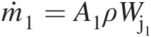
Specific angular momentum: R1Vθ1 = R1(R1Ω + Wj1)R1Vθ1=R1R1Ω+Wj1
Outflow rate of angular momentum: Ḣ1=ṁ1R1R1Ω+Wj1
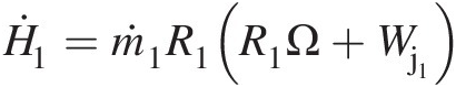


Outlet 2
Mass flow rate: ṁ2=A2ρWj2
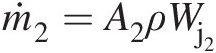
Specific angular momentum: R2Vθ2 = R2(R2Ω − Wj2)R2Vθ2=R2R2Ω−Wj2
Outflow rate of angular momentum: Ḣ2=ṁ2R2R2Ω−Wj2
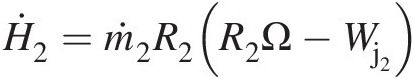


Because the friction torque will act in the clockwise direction (opposite to the sprinkler arm rotation), the angular momentum equation yields


Example 2.3
Figure 2.31 shows a high-pressure rotary arm with three nozzles for air impingement cooling of a cylindrical surface. Air at total pressure of 3 bar3bar and total temperature of 507.5 K507.5K exits each nozzle. The ambient pressure outside the rotary arm is 1 bar1bar. At the maximum RPM, the rotary arm needs to overcome a frictional torque of 12.5 Nm12.5Nm. For the given geometric data, calculate the maximum RPM of the rotary arm. Note that each air nozzle operates under choked flow condition with identical jet velocity relative to the rotary arm. Assume κ = 1.4κ=1.4 and R = 287 J/(kg K)R=287J/kgK for air. The geometric data are: jet diameter (dj) = 7 mm, R1 = 0.50 m,(dj)=7mm,R1=0.50m, R2 = 1 mR2=1m, and R3 = 1.40 mR3=1.40m.

Solution
Mass flow rate through each air nozzle:
Jet area: Aj=πdj24=π0.00724=3.8485×10⁻⁵m2
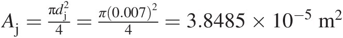
Total pressure flow function at M = 1M=1: Fft∗ = 0.0404Fft∗=0.0404
ṁ=AjFft∗PtTt=3.8485×10−5×0.0404×300000134.5+273=0.0231kg/s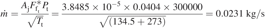


Air jet velocity relative to the rotary arm:
Static temperature at the nozzle throat: Ts∗=2Ttκ+1=2×407.51+1.4=339.6K
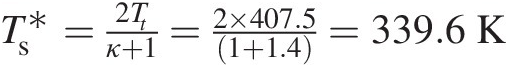
For the choked flow through each nozzle, M = 1M=1, giving
Wj=κRTs∗=1.4×287×339.6=369.384m/s


Torque and angular momentum balance on the rotary arm control volume:
Absolute jet velocity contributing to the angular momentum flux at any radius is computed by
Net efflux of angular momentum in the counterclockwise direction

Torque as a result of pressure force acting on the fluid control volume in the counterclockwise direction:

where

If Torquearm – to – fluidTorquearm-to-fluid, the torque from the rotary arm, is acting in counterclockwise direction on the fluid control volume, then the torque-angular-momentum balance yields the following equation


At the maximum RPM, the net torque acting on the rotary arm must be zero, i.e.,
Thus,


Giving

Rotary arm maximum RPM = 473.6RPM=473.6
Example 2.4
Figure 2.32 shows an ejector pump used in many engineering applications. Describe the working principle of this pump. Making any simplifying assumptions, determine the ratio Q2/Q1Q2/Q1.

Solution
The operating principle of an ejector pump schematically shown in Figure 2.32 is rather simple. The volumetric flow rate Q1Q1 in the convergent nozzle A enters the suction chamber B at a very high velocity. As a result, the static pressure of the stream as well the whole suction chamber drops considerably. This drop in static pressure in the chamber creates a suction pressure inducing the volumetric flow rate Q2Q2 in pipe O. The role of diffuser C is to allow the total volumetric flow rate Q1 + Q2Q1+Q2 to exhaust at the ambient pressure with a subambient static pressure in chamber B.
For the present analysis, let us assume that the fluid of the nozzle flow is identical to that of the pumped (induced) flow with constant density ρρ. For a total supply pressure of Pt1Pt1, we can express the extended Bernoulli equation governing the nozzle flow from its inlet to outlet as


where K1K1 is the minor loss coefficient in the nozzle based on its exit velocity V1V1, and PsBPsB is the subambient static pressure in chamber B.
Similarly, the extended Bernoulli equation for the induced flow from the ambient conditions yields

Combining the aforementioned equation with the one previously obtained for the nozzle flow yields


where A1A1 and A2A2 are the nozzle throat area and pipe area, respectively. By simplifying the aforementioned equation, we obtain


where

Example 2.5
Figure 2.32 shows a diverging duct whose diameter varies linearly from 0.1 m to 0.2 m over a length of 1.0 m. If the Darcy friction factor for the entire duct is constant at 0.005, find the major head loss as a result of friction within the duct for a volumetric flow rate of 1.0 m3/s.
Solution
Using the Darcy friction factor, the pressure loss as a result of friction in the fully developed flow in a circular duct of diameter D and length L can be written as

which in terms of the volumetric flow rate QQ becomes

In terms of major head loss, we can write the aforementioned equation as

Note that, for a given volumetric flow rate, the major head loss in the duct flow is independent of the fluid density.
For the diverging duct shown in Figure 2.33, the diameter increases in the flow direction, say the xx direction. Assuming x = 0x=0 at duct inlet, we can obtain its diameter at any xx by the following equation:

Noting that the component of the wall shear force along the flow direction is responsible for the frictional pressure loss in the diverging duct, we can express the differential major head loss over the differential duct length dxdx as

Substituting D = 0.1(1 + x)D=0.11+x in the aforementioned equation and integrating over the entire duct length, we obtain


Example 2.6
Figure 2.34 shows an isentropic flow of air in a rubber pipe of constant-diameter 0.100 m0.100m with the inlet total pressure and total temperature of 1.2 bar1.2bar and 300 K300K, respectively. The ambient pressure is 1.0 bar1.0bar. The pipe is slowly deformed into a convergent-divergent nozzle, shown by the dotted line, until the flow just chokes (M = 1.0M=1.0) at the throat. For the given boundary conditions, calculate the throat diameter. Assume air as a perfect gas with κ = 1.4κ=1.4 and R = 287 J/(kg K)R=287J/kgK.

Solution
- Area at pipe inlet and exit:
Ainlet=Aexit=πDexit24=π0.124=7.854×10⁻³m2
- Pressure ratio at pipe exit:
PtexitPsexit=PtexitPamb=1.21.0=1.2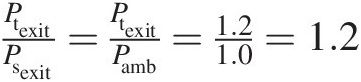
- Exit Mach number MexitMexit:
TtexitTsexit=PtexitPsexitκ−1κ=1.20.286=1.0535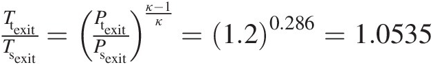


which yields

Mass flow rate through the pipe:


Throat diameter: For the choked flow at the throat, we have Mthroat = 1.0Mthroat=1.0 and F̂ft∗=0.6847 , giving

Example 2.7
Figure 2.35 shows air flow in a convergent-divergent (C-D) nozzle. A normal shock stands in the divergent section. The exit-to-throat area ratio Aexit/AthroatAexit/Athroat of the C-D nozzle is known. For the given exit Mach number MexitMexit, write a step-by-step nongraphical and noniterative procedure to determine the ratio of nozzle area ANSANS to the throat area A∗A∗ at the normal shock location.

Solution
Step 1: For the given value of MexitMexit, use isentropic flow Table A.2 of Sultanian (2015) to determine Aexit/A2∗
 .
.
Step 2: Because A1∗=A∗
 , calculate the ratio A1∗/A2∗
 as
as
A1∗A2∗=AexitA2∗AexitA1∗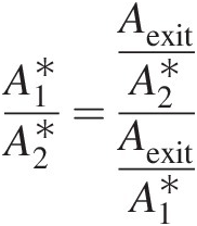
Step 3: Because the mass flow rate and total temperature remain constant across a normal shock, we can write A1∗/A2∗=Pt2/Pt1
 ; the flow on the either side of the normal shock is isentropic.
Step 4: Knowing Pt2/Pt1Pt2/Pt1, find M1M1 and M2M2 from the normal shock Table A.6 of Sultanian (2015)
Step 5: Use M1M1 to find ANS/A1∗
 from the isentropic flow Table A.2 of Sultanian (2015)


Example 2.8
In an attempt to reduce the heat loss from a metal hot-water tube of outer radius 6.5 mm6.5mm, a plumber decides to insulate the water line with 12 mm12mm thick insulation having thermal conductivity of 0.156 W/(m K)0.156W/mK. As a result of the high heat transfer coefficient between water flow and metal pipe and the high thermal conductivity of the metal, the entire metal pipe can be considered to remain at a uniform temperature of 350 K350K. The tube is surrounded by air at 300 K300K, for which h = 9.0 W/(m2 K)h=9.0W/m2K. In terms of percentage, how successful is the plumber in reducing the heat loss?
Solution
Let us compute the heat transfer rate per unit length of the tube, when it is bare (without insulation) and with insulation in place.


It is interesting to note that by insulating the tube, heat transfer increased by 34.5 percent; one would expect it to decrease. This situation is commonly known as the plumber paradox. The critical outer radius in this case is given by rc = k/h = 0.156/9 = 0.01733rc=k/h=0.156/9=0.01733, which corresponds to the maximum heat transfer from the insulated tube. It can be easily verified that, for the heat transfer from the insulated tube to be lower than that from a bare tube, the insulation thickness must be more than 67.5 mm.
Example 2.9
Figure 2.36 shows the rectangular cross-section of a plate, which is very long in the normal direction along which no property varies. As shown in the figure, one end of the plate is held at a constant temperature T0T0 and the opposite end remains adiabatic (q̇=0 ). The bottom of the plate is heated with a uniform heat flux q̇1
 and the top side is subject to convective boundary condition with constant heat transfer coefficient hh and fluid temperature TfTf. The Bio number (Bi = ht/kBi=ht/k) is small enough that any temperature variation along the plat thickness may be neglected. The uniform volumetric heat generation rate within the plate equals ṡ
 . Find an analytical solution to compute plate temperature variation in the xx direction, that is, find T = T(x)T=Tx.

Figure 2.36 One-dimensional temperature variation in a rectangular plate with mixed boundary conditions and uniform volumetric heat generation (Example 2.9).
Solution
Assuming unit plate length in the normal direction, the energy balance over the control volume between xx and x + Δxx+Δx yields


Using Fourier’s law of heat conduction and simplifying the resulting expression, we finally obtain

where

With the boundary conditions θ = 1θ=1@ξ = 0ξ=0 and dθ/dξ = 0dθ/dξ=0@ξ = 1ξ=1, the solution of the aforementioned second-order homogeneous ordinary differential equation can be easily obtained as

Problems
2.1 Consider an incompressible flow through a constant-area circular pipe with negligible wall friction. At the inlet, the pipe is connected to a plenum maintained constant pressure. At the outlet, the flow is discharged at the fixed ambient pressure. If a short ideal conical diffuser is appended to the pipe at its outlet, will the mass flow rate increase, decrease, or remain constant? How will your answer change for a compressible flow with subsonic and supersonic conditions at the pipe exit?
2.2 Based on how the static and total pressures vary in an adiabatic diffuser, shown in Figure 2.37, will the flow in the bypass duct occur from A to B or from B to A? Explain your reasoning.

Figure 2.37 Flow direction in the bypass duct of an adiabatic diffuser (Problem 2.2).
2.3 For an incompressible flow through a variable-area duct, which is frictionless and rotates at a constant angular velocity, show that the change in total pressure relative to the duct equals the change in static pressure as a result of rotation alone, with no change in flow area.
2.4 Figure 2.38 shows steady water flow through a vertical pipe of radius RR. A fully developed laminar flow with a parabolic velocity profile prevails at section 1. The flow transitions to a fully-developed turbulent flow with the 1/7th power-law profile at section 2. Over the pipe length LL, the total shear force and gravitational body force correspond to FfFf and WgWg, respectively. For the mass flow rate ṁ through the pipe, the static pressure at sections 1 and 2 are Ps1Ps1 and Ps2Ps2, respectively. Express the total shear force FfFf in terms of other known quantities.

Figure 2.38 Steady flow of water through a vertical pipe (Problem 2.4).
2.5 Figure 2.39 shows an incompressible flow in a sudden pipe expansion with the upstream pipe diameter D1D1 and downstream pipe diameter D2D2. The laminar flow in the upstream pipe is fully developed with a parabolic velocity profile. The flow exiting the larger pipe is turbulent, which is assumed to have a uniform velocity profile. The static pressure at both sections 1 and 2 is assumed to be uniform. Neglecting any shear stress on the downstream pipe wall, find the change in both static pressure and total pressure between sections 1 and 2 of this flow system.

Figure 2.39 Sudden expansion pipe flow with a parabolic velocity profile at inlet and uniform velocity at outlet (Problem 2.5).
2.6 Figure 2.40 shows impingement air cooling of a cylindrical surface using a high-pressure rotary arm fitted with identical nozzles. Each nozzle is choked with equal mass flow rate ṁ and exit static pressure Ps∗
 , which is higher than the ambient pressure PambPamb. At the maximum rotational velocity ΩΩ, the rotary arm needs to overcome a frictional torque ΓfΓf. Derive an expression to calculate ΩΩ.

Figure 2.40 Impingement air cooling of a cylindrical surface (Problem 2.6).
2.7 As shown in Figure 2.41, two air streams of different properties enter a long duct with the cross-sectional area of 0.002 m20.002m2. At section 1 (inlet), the hotter stream forms the central core and is surrounded by the colder stream. Each stream occupies equal area (neglect the wall thickness of the inner duct). The uniform static pressure at section 1 equals 895614 Pa895614Pa and that at section 2 (outlet) equals 10 bar10bar. The total pressure and total temperature of each stream at section 1(inlet) are given later. Both streams are assumed to have been fully mixed before exiting the duct at section 2 with uniform properties.
| Stream 1 | Stream 2 | |
|---|---|---|
| Total Temperature (K) | 1173 | 1473 |
| Total Pressure (bar) | 10 | 15 |
Assuming κ = 1.4κ=1.4 and R = 287 J/(kg K)R=287J/kgK, calculate:
(a) Mass flow rate of each stream
(b) Section-average total temperature and static temperature at inlet
(c) Section-average total pressure at inlet
(d) Percentage drop in total pressure from inlet to outlet
(e) Total wall shear force acting on the flow between inlet and outlet

Figure 2.41 Mixing of two compressible flows in a duct (Problem 2.7).
2.8 Figure 2.42 shows a high-pressure inlet bleed heat system (IBH) of a land-based gas turbine used for power generation. When the ambient air is cold, the inlet bleed heat system is used to raise its temperature to prevent ice formation on the compressor IGV’s (inlet guide vanes). In this system, the hot air is bled from an intermediate compressor stage and mixed uniformly with air flow at the engine inlet. Let’s consider such a system. The ambient pressure and temperature are 1 bar1bar and 293 K293K, respectively. The Mach number of the air flow entering the IGV is 0.60.6. To prevent ice formation, the static temperature at this section is required to be 275 K275K. The air mass flow rate entering the engine inlet system (before the high-pressure bleed heat section) at a low Mach number (M < 2M<2) is 275 kg/s. The total temperature and pressure of the air bled from the compressor are 542 K542K and 8 bar8bar, respectively. Neglect any changes in the pressure and temperature in the bleed air supply system. Assuming air as a perfect gas with κ = 1.4κ=1.4 and R = 287 J/(kg K)R=287J/kgK:
(a) Calculate the mass flow rate of the compressor bleed air to achieve the design objective at compressor IGV inlet
(b) To promote uniform mixing of the hot compressor bleed air with the cold inlet ambient air, 200 nozzles for the bleed air injection are uniformly placed in the inlet duct cross-section. Find the effective flow area of each nozzle.

Figure 2.42 High-pressure inlet bleed heat (IBH) system of a land-based gas turbine power plant (Problem 2.8).
2.9 In a land-based gas turbine used for power generation, the turbine exhaust enters an annular diffuser, shown in Figure 2.43, at the total-velocity Mach number of 0.60 and the total temperature of 723 K723K. The swirl velocity (tangential velocity) at the diffuser inlet equals15 percent of the total velocity. The flow exits the diffuser fully axially at a Mach number of 0.15 with no change in total temperature. The design calls for the static pressure at the diffuser exit to be 1.018 bar1.018bar to allow the exhaust gases to discharge into the ambient air via a downstream duct system (not shown in the figure). The exit-to-inlet flow area ratio for the annular diffuser is 3.45. Find the pressure rise coefficient (CPCP) for the annular diffuser. If the last stage turbine is redesigned for zero swirl velocity at its exit, how will the pressure rise coefficient of the annular diffuser change? Assume exhaust gases with κ = 1.4κ=1.4 and R = 287 J/(kg K)R=287J/kgK.

Figure 2.43 Exhaust diffuser of a land-based gas turbine for power generation (Problem 2.9).
2.10 An isentropic convergent-divergent nozzle having an area ratio (exit area/throat area) of 2 discharges air into an insulated pipe of length LL and diameter DD. The nozzle inlet air has the stagnation pressure of 7 × 10⁵Pa7×105Pa and the stagnation temperature of 300 K300K, and the pipe discharges into a space where the static pressure is 2.8 × 10⁵Pa2.8×105Pa. Calculate fL/DfL/D of the pipe and its mass flow rate per unit area for the cases when a normal shock stands: (a) at the nozzle throat, (b) at the nozzle exit, and (c) at the pipe exit.
2.11 A normal shock is detected in a convergent-divergent nozzle with the given exit-to- throat area ratio, inlet total pressure, and inlet total temperature. The air flow is isentropic on either side of the normal shock. For the given exit static temperature, write a noniterative, nongraphical step-by-step procedure to determine the ratio of the nozzle flow area, where the normal shock is located, to the nozzle throat area. Assume κ = 1.4κ=1.4 and R = 287 J/(kg K)R=287J/kgK for air.
2.12 A supersonic air-flow with known total pressure, total temperature, and static pressure enters a pipe of given constant diameter and constant friction factor. With its adiabatic and stationary wall, the pipe is 15 percent longer than the maximum needed to achieve the choked flow conditions (frictional choking). While the flow remains choked, a normal shock occurs within the pipe. Write a step-by-step procedure to determine the location (the distance from the pipe inlet) of the normal shock. Assume air to be a perfect gas with κ = 1.4κ=1.4 and R = 287 J/(kg K)R=287J/kgK.
2.13 A normal shock is detected in a convergent-divergent nozzle with known exit-to-throat area ratio, inlet total pressure, and inlet total temperature. The air flow is isentropic on either side of the normal shock. For a given exit static temperature, write a noniterative, nongraphical step-by-step procedure for finding the nozzle area ratio (ratio of nozzle area to throat area) that corresponds to the normal shock location. For air, assume κ = 1.4κ=1.4 and R = 287 J/(kg K)R=287J/kgK.
2.14 Derive a relationship between the loss coefficient KK and the discharge coefficient CdCd for an incompressible flow in a sudden pipe expansion with the larger-to-smaller area ratio A2/A1A2/A1.
2.15 For both radially inward and outward flows through two counterrotating disks, derive relevant equations to compute windage temperature rise between two radial locations. Assume both disks to be adiabatic (zero heat transfer). List all your assumptions.
References
Bibliography
Nomenclature
- AA
Flow area
- ATEX
Atmosphères Explosibles
- AcAc
Area of Vena contracta
- A→

Flow area vector
- cc
Specific heat of solid
- cpcp
Specific heat of gas at constant pressure
- cvcv
Specific heat of gas at constant volume
- CC
Speed of sound
- CdCd
Discharge coefficient
- CfCf
Shear coefficient or Fanning friction factor
- CpCp
Diffuser pressure rise coefficient
- DD
Pipe diameter
- ff
Moody or Darcy friction factor
- ee
Specific total energy of a system
- êr

Unit vector in the radial direction
- EE
Total energy of a system
- EkEk
Ekman number (Ek=μ/ρΩLref2
 )
)
- FF
Total force
- F→

Force vector
- FfsFfs
Static-pressure mass flow function with dimensions of R

- F̂fs

Dimensionless static-pressure mass flow function
- FftFft
Total-pressure mass flow function with dimensions of R

- F̂ft

Dimensionless total-pressure mass flow function
- gg
Acceleration as a result of gravity
- GrGr
Grashof number (Gr = gβ(ΔT)L3ρ2/μ2Gr=gβΔTL3ρ2/μ2)
- hh
Specific enthalpy; heat transfer coefficient; height from a datum
- HH
Angular momentum
- H→

Angular momentum vector
- H⇀̇

Angular momentum flow rate
- II
Rothalpy; current
- IfsIfs
Static-pressure impulse function
- IftIft
Total-pressure impulse function
- kk
Thermal conductivity
- KK
Loss coefficient
- KEKE
Kinetic energy
- LrefLref
Reference length scale
- mm
Mass
- ṁ

Mass flow rate
- MM
Mach number; linear momentum
- M→

Linear momentum vector
- M→̇

Linear momentum flow rate
- MθMθ
Rotational Mach number (Mθ=rΩ/κRTs)
- NN
Normal shock function
- N∞N∞
Asymptotic value of NN as M→∞M→∞
- NinNin
Number of inlets
- NuNu
Nusselt number
- NoutNout
Number of outlets
- PP
Pressure
- PiPi
Impulse pressure
- P˜

Reduced pressure
- PdcomPdcom
- PdincPdinc
Incompressible dynamic pressure
- PdratioPdratio
Ratio of compressible dynamic pressure to incompressible dynamic pressure
- Ṗentropy
Rate of entropy production
- PEPE
Potential energy
- qq
Specific heat transfer
- q̇

Heat flux
- q̇→

Heat flux vector
- QQ
Heat transfer; volumetric flow rate
- Q̇

Heat transfer rate; cycle heat rate
- rr
Cylinder polar coordinate rr
- r→

Position vector from the origin (rotating coordinate system)
- r∗r∗
Recovery factor
- RR
Gas constant; radial distance; resistance
- ReRe
Reynolds number
- RoRo
Rossby number Ro = Wref/ΩLref(Ro=Wref/ΩLref)
- ss
Specific entropy
- ṡ

Volumetric heat generation rate
- SS
Entropy
- SfSf
Swirl factor
- STST
Stream thrust
- tt
Time; thickness
- TT
Temperature
- TfTf
Reference fluid temperature
- uu
Specific internal energy
- UU
Total internal energy of a system; rotor tangential velocity
- UiUi
Velocity in tensor notation
- v

Specific volume
- VV
Total absolute velocity; voltage
- V→

Absolute velocity vector
- V

Volume
- ww
Specific work transfer
- WW
Total relative velocity; work transfer; weight
- W→

Relative velocity vector
- Ẇ

Rate of work transfer (power)
- WrefWref
Reference relative velocity scale
- xx
Cartesian coordinate xx; axial direction
- xixi
Cartesian coordinates in tensor notation
- yy
Cartesian coordinate yy
- zz
Cartesian coordinate zz
- ZZ
Complex velocity


Subscripts and Superscripts
- awaw
Adiabatic wall
- BB
Body
- barebare
Without insulation
- com
Compressible
- cond
Conduction
- conv
Convection
- cyclecycle
Thermodynamic cycle
- CC
Compressor
- CSCS
Control system
- CVCV
Control volume
- CCTCCT
Coupling correction term
- CVSCVS
Control volume surface
- DD
Duct
- ff
Fluid; friction
- fcfc
Forced convection
- F1 − 2F1−2
Radiation view factor between surfaces 1 and 2
- gg
Gravity
- i
Isentropic; impulse
- in
Inlet
- inc
Incompressible
- ins
With insulation
- irrev
Irreversible
- m
Metal; material
- max
Maximum
- ncnc
Natural convection
- net
Net (turbine work output minus compressor work input)
- out
Outlet
- p
Polytropic
- rr
Component in rr coordinate direction
- rad
Radiation
- ref
Reference
- rev
Reversible
- RR
Rotor reference frame
- ss
Static
- SS
Stator reference frame; surface
- shsh
Shear
- tt
Total
- TT
Turbine
- thth
Thermal
- ww
Wall
- xx
Component in xx coordinate direction
- yy
Component in yy coordinate direction
- zz
Component in zz coordinate direction
- ∞∞
Free stream; asymptotic value for M→∞M→∞
- θθ
Component in θθ direction
- ∗∗
Value at sonic condition (M = 1M=1)
Greek Symbols
- αα
Thermal diffusivity α = k/(ρc)(α=k/ρc)
- ββ
Isobaric compressibility of fluid
- εε
Surface emissivity
- ΓΓ
Torque
- Γ→

Torque vector
- ζ→

Vorticity vector
- ηη
Efficiency; number of transfer units (NTU): η=πDhL/(ṁcp)
- θθ
Cylindrical polar coordinate θθ; dimensionless temperature
- θ˜

Angle between resultant velocity and tangential velocity within Ekman boundary layer
- κκ
Ratio of specific heats κ = cp/cv(κ=cp/cv)
- λλ
Second coefficient of viscosity
- μμ
- νν
Kinematic viscosity (ν = μ/ρν=μ/ρ)
- ξξ
Dimensionless similarity variable
- ππ
Pressure ratio
- ΠΠ
Change agent
- ρρ
Density
- σσ
Stefan-Boltzmann constant
- ττ
Shear stress
- ΦΦ
Extensive general property
- ϕϕ
Intensive general property
- ω→

Local rotation vector
- ΩΩ
Rotational velocity around axial direction
- Ω→

Rotational velocity vector


