3.0 Introduction
The main objective of an engineering analysis is to have the prediction results as close to the physical reality as possible. These results are said to be numerically accurate if the modeling equations are solved correctly. They are considered physically accurate if they also correctly predict the physical reality, which is independent of the method of analysis. In general, for prediction results to be physically accurate, they ought to be numerically accurate. In the context of computer code (design tool) development, the numerical accuracy of the computed results is ensured through code verification, and their physical accuracy is determined by code validation. In our discussion, we will tacitly assume that the computational method used for solving a flow network ensures numerical accuracy. The accuracy in the present context essentially means physical accuracy.
The physics-based one-dimensional (1-D) thermofluids modeling of various components of internal flow systems of a gas turbine is a design necessity, offering the best compromise of prediction accuracy, speed, and cost. Predictions are generally made using complex flow networks of these components in all three design phases: conceptual, preliminary, and detailed. The reliability of design predictions depends in large part on the company-proprietary empirical correlations. Each robust design is performed with compressible flow networks in a short available design cycle time. The CFD technology is leveraged in two ways; first, to develop a better understanding of the component flow physics, reinforcing its 1-D modeling, and second, to delineate areas of design improvement in the detailed design phase using an entropy map. In this chapter, we limit our discussion to steady compressible flow networks with the possibility of internal choking and normal shocks.
The accuracy of results from a flow network primarily depends upon two factors: (1) the core formulation that ensures that the conservation laws of mass, momentum, energy, and entropy are duly satisfied for each flow element and junction in the network and (2) the empirical correlations, which are based on the benchmark quality data, are representative of the physical reality. While there is always a need for improved empirical correlation for an existing or newly designed element, the core mathematical formulation based on the established laws of flow and heat transfer physics ought to remain invariant. Accordingly, the physics-based modeling in the context of our discussion in this chapter will imply that all the conservation laws are fully satisfied in the flow network. Thus, any lack of accuracy of a network solution can be entirely attributed to the deficiencies in one or more empirical correlations used in the network.
3.1 1-D Flow Modeling of Components
The physics-based 1-D flow modeling of each component of gas turbine internal flow systems is achieved through large control volume analysis of the conservation equations of mass, momentum, energy, and entropy. For a compressible flow, the momentum equation remains coupled with the energy equation through density, which is computed using the equation of state of a perfect gas. In this chapter, we present the modeling of a duct and an orifice, which are two basic components of an internal flow system. Modeling of other special components, such as vortex, rotor-rotor and rotor-stator cavities, and seals are presented in the following chapters.
3.1.1 Duct with Area Change, Friction, Heat Transfer, and Rotation
In this section, we present the most general modeling of one-dimensional compressible flow in a variable-area duct with wall friction, heat transfer, and rotation (constant angular velocity) about an axis different from the flow axis. The modeling methodology also allows for the presence of internal choking (M = 1M=1) and normal shock, which features abrupt changes in flow properties. In the present approach, the long duct is divided into multiple control volumes, which are serially coupled such that the outlet flow properties of one control volume become the inlet flow properties for the downstream one. In each control volume, wall boundary conditions are assumed uniform, although they may vary over different control volumes. Thus, in order to model the entire duct, we need to develop modeling equations only for a representative control volume, as has been done in the following sections.
3.1.1.1 Mass Conservation (Continuity Equation)
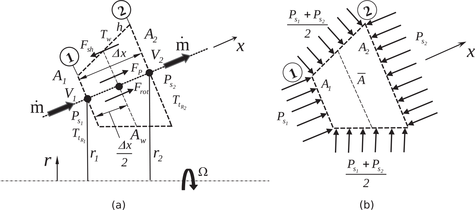
For the duct control volume shown in Figure 3.1, the velocity, density, and area for the x-direction flow are assumed to vary linearly from inlet (section 1) to outlet (section 2). For a steady flow through the control volume, the mass conservation yields
 (3.1)
(3.1)where
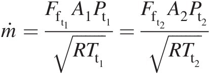
In terms of the total pressure, total temperature, Mach number, and total-pressure mass flow function (presented in Chapter 2), we can compute mass flow rate at the duct control volume inlet and outlet as
3.1.1.2 Linear Momentum Equation
For the duct control volume shown in Figure 3.1a, we can write the steady flow momentum equation as
 (3.2)
(3.2)where
FP≡FP≡ Pressure force acting on the control volume in the momentum direction
Fsh≡Fsh≡ Shear force acting on the control volume opposite to the momentum direction
Frot≡Frot≡ Rotational body force acting on the control volume in the momentum direction
Let us now evaluate the surface forces due to static pressure and wall shear and the body force due to rotation.
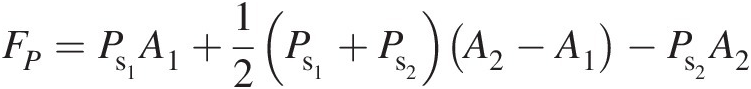
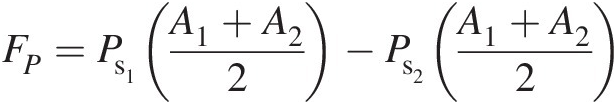
Pressure force (FPFP). Figure 3.1b shows the static pressure distribution on the duct control volume, where we have assumed that the average pressure on the lateral surfaces is the average of inlet and outlet pressures. The total pressure force in the x direction, resulting from the surface pressure distribution, can be expressed as
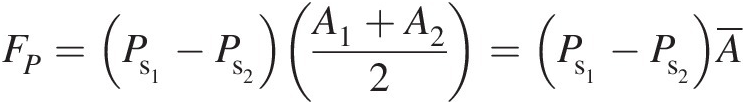 (3.3)
(3.3)Equation 3.3 shows that the net force resulting from a pressure distribution on the duct control volume with area change in the flow direction is the product of the difference in the inlet and outlet pressures and the mean flow area.
Shear force (FshFsh). The net shear force acting on the control volume in the momentum direction can be expressed as
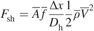 (3.4)
(3.4)where f¯ is the average value of the Darcy friction factor over the lateral control volume surface.
Rotational body force (FrotFrot). The component of the rotational body force acting on the control volume in the momentum direction can be expressed as
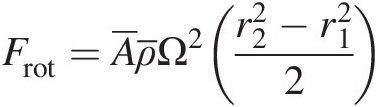 (3.5)
(3.5)Substituting the foregoing expressions for the pressure force, shear force, and rotational body force in Equation 3.2, we obtain
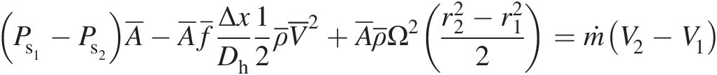
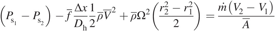 (3.6)
(3.6)Thus, knowing Ps1Ps1 at the inlet, we can use Equation 3.6 to compute the static pressure Ps2Ps2 at the outlet as
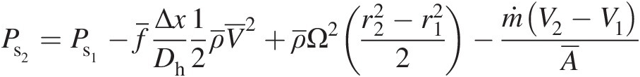
In Equation 3.7, the terms representing changes in static pressure due to friction, rotation, and momentum-change are given as follows:
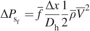 (3.8)
(3.8)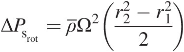 (3.9)
(3.9) (3.10)
3.1.1.3 Energy Equation
The steady flow energy equation for the duct control volume involves heat transfer at the wall and work transfer due to rotation. Both of these energy exchanges result in change in gas total temperature from inlet to outlet. It is important to note that, while the rotational work transfer does not depend upon the simultaneous heat transfer, the heat transfer does depend upon the simultaneous work transfer. This work transfer changes the gas total temperature and hence the difference between the wall temperature and the adiabatic wall temperature, affecting heat transfer. Sultanian (2015) provides a closed-form analytical solution for the coupled heat transfer and rotational work transfer in a compressible duct flow, including a correction term if one decides to simply add the separately-computed changes in gas total temperature due to heat transfer and rotation. Thus, the gas total temperature at the exit of the flow element with rotation can be computed as
where
(ΔTtR)HT≡ΔTtRHT≡ Change in gas total temperature due to heat transfer
(ΔTtR)rot≡ΔTtRrot≡ Change in gas total temperature due to rotation
(ΔTtR)CCT≡ΔTtRCCT≡ Heat transfer and rotational work transfer coupling correction term
Heat transfer: (ΔTtR)HTΔTtRHT. For the convective heat transfer, we assume that the duct control volume walls are isothermal (constant wall temperature TwTw) and the heat transfer coefficient h, which is either specified or computed from an empirical correlation, remains constant from inlet to outlet. We further assume that the adiabatic wall temperature at each section of the control volume equals the gas total temperature, implying a recovery factor of 1.0.
Based on the analysis presented in Chapter 2, the change in gas total temperature due to heat transfer from inlet to outlet can be expressed as
where
Rotational work transfer: (ΔTtR)rotΔTtRrot. When the gas enters a rotating duct, it assumes the state of solid body rotation, that is, the gas starts rotating at the constant angular velocity of the duct. Under adiabatic conditions, the change in gas total temperature (relative to the control volume rotating at constant speed) between two radial locations can be obtained by equating gas rothalpy (see Chapter 2) at these locations. Thus, we can write
 (3.13)
Coupling Correction Term: (ΔTtR)CCTΔTtRCCT. Sultanian (2015) derived the heat transfer and rotational work transfer coupling correction term as
 (3.14)
3.1.1.4 Internal Choking and Normal Shock Formation
Compressible flow in a variable-area duct, for example in a convergent-divergent nozzle, can feature internal choking at a section where the flow velocity equals the local speed of sound (M = 1M=1). If the flow area increases beyond this section, the flow becomes supersonic with the possibility of a normal shock if the duct exit conditions are subsonic. The flow properties vary continuously across a section where the flow is choked; however, they vary abruptly across a normal shock. In the modeling of a long variable-area duct, a good way to simulate the choked-flow section is to make it coincide with an interface between adjacent control volumes. For simulating a normal shock, however, it is better to imbed a negligibly thin control volume within which the normal shock occurs. Using the normal shock equations presented in Chapter 2, we can then compute the properties at the outlet of this imbedded control volume.
3.1.1.5 Flexibility of Duct Flow Modeling
The comprehensive 1-D modeling of a duct flow presented in the foregoing is much more versatile that it first appears. An orifice can also be simulated using a short duct with no area change and with specified discharge coefficient CdCd such that the mass flow rate through the orifice (duct) can be computed using the equation
 (3.14)
In Equation 3.14, the flow properties correspond to the mechanical area A that yields the effective area Aeff = CdAAeff=CdA. The total-pressure mass flow function F̂ft is a function of Mach number, which is uniquely computed from the isentropic pressure ratio at A. In terms of the static-to-total pressure ratio Ps/PtPs/Pt, we can write Equation 3.14 as
 (3.15)
which holds good for 0.5283 ≤ Ps/Pt < 10.5283≤Ps/Pt<1 where Ps/Pt = 0.5283Ps/Pt=0.5283 corresponds to the choked flow condition (M = 1M=1) for air with κ = 1.4κ=1.4.
The discrete duct flow modeling presented in this section can also be used to simulate and be validated against the duct flow with each separate effect presented in Chapter 2, namely, isentropic flow with area change (without the friction, heat transfer, and rotation), Fanno flow (without the area change, heat transfer, and rotation), and Rayleigh flow (without the area change, friction, and rotation). We can certainly simulate any combination of various effects on the duct flow. It is interesting to note that a rotating duct flow can also be used to simulate a forced vortex.
3.1.2 Orifice
Orifices are the most ubiquitous element of a gas turbine internal flow system. They are used in both stationary and rotating components either to restrict the flow or to meter it. A choked-flow (M = 1M=1) orifice designed with negligible vena contra can be used as a device with constant mass flow rate, not affected by downstream flow conditions. For constant source and discharge pressures in a passive bleed flow line, orifices in the form of short nozzles are generally used to obtain the desired flow rate. Valves may be modeled as a variable-area orifice.
3.1.2.1 Sharp-Edged Orifice
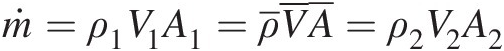
Figure 3.2a shows a sharp-edged orifice in which the flow through the orifice area at section 2 is driven by the upstream total pressure at section 1 and the downstream static pressure at section 3. Due to flow contraction at the orifice, the flow initially converges to a smaller area, called vena contracta, before expanding to the larger downstream area. The area (AvcAvc) of the vena contracta is a strong function of A3/A2A3/A2, but it does not depend on the pressure ratio across it for an incompressible flow. The overall loss in the total pressure between sections 1 and 3 mainly results from the sudden-expansion loss downstream of the vena contracta. Using the control volume analysis of an incompressible flow, this loss is calculated to be the dynamic pressure of the difference in velocities at the vena contracta and section 3.
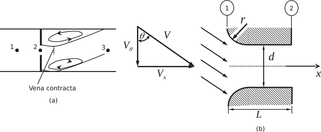
Figure 3.2 (a) Sharp-edged orifice and (b) parameters influencing orifice discharge coefficient.
For a compressible flow, there are essentially two approaches to compute mass flow rate through a sharp-edged orifice. The first approach (a classical one) is based on an extension of the incompressible flow method and is given by (see Benedict (1980))
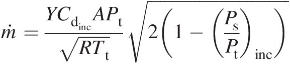 (3.16)
where Y is called the adiabatic expansion factor to account for the decrease in density as the flow expands (static pressure decreases) in a compressible flow. Buckingham (1932) proposed the following empirical relation for computing Y:
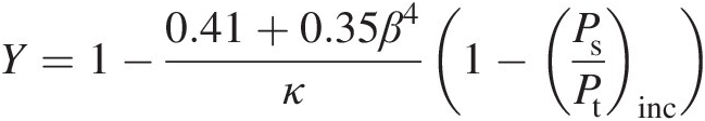 (3.17)
where β is the ratio of orifice diameter to housing pipe diameter. Parker and Kercher (1991) recommended the use of Equation 3.17 for 0.63 ≤ (Ps/Pt)inc ≤ 10.63≤Ps/Ptinc≤1 and 0 ≤ β ≤ 0.50≤β≤0.5, and for 0 ≤ (Ps/Pt)inc ≤ 0.630≤Ps/Ptinc≤0.63, they proposed the following semi-empirical equation:
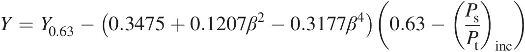 (3.18)
where Y0.63Y0.63 is computed from Equation 3.17 with (Ps/Pt)inc = 0.63Ps/Ptinc=0.63.
To compute the incompressible flow discharge coefficient CdincCdinc used in Equation 3.15, Stolz (1975) proposed the following “universal” equation:
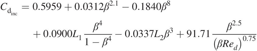 (3.19)
where
L1≡L1≡ Dimensionless upstream pressure-tap location with respect to the orifice upstream face
L2≡L2≡ Dimensionless downstream pressure-tap location with respect to the orifice downstream face
Red≡Red≡ Reynolds number based on the orifice diameter
The main motivation behind using the foregoing approach in calculating the mass flow rate of a compressible flow through a sharp-edged orifice is to leverage the vast amount of incompressible flow data available for CdincCdinc. In addition, as discussed next, the method also captures the compressibility effect as the downstream static pressure decreases beyond the nominal choking at the vena contracta, increasing its area with pressure ratio. This results in a higher mass flow rate beyond the critical pressure ratio under the same upstream stagnation conditions.
The second approach, which will be used in this book, to calculating compressible mass flow rate through a sharp-edged orifice is to use Equation 3.15. From Equations 3.15 and 3.16, we can compute the discharge coefficient CdCd as
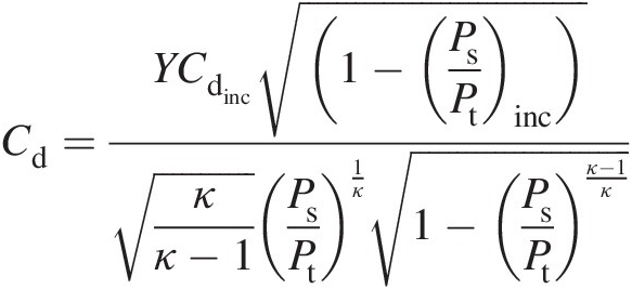 (3.20)
Note that in the numerator of Equation 3.20, 0 ≤ (Ps/Pt)inc ≤ 10≤Ps/Ptinc≤1 while in the denominator we have 0.5283 ≤ Ps/Pt < 10.5283≤Ps/Pt<1, which means the denominator of this equation has a maximum value of 0.6847 that corresponds Ps/Pt = 0.5283Ps/Pt=0.5283.
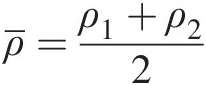
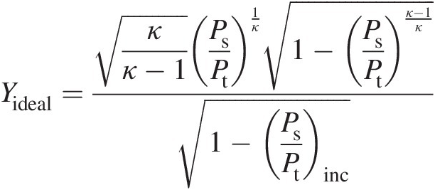
Figure 3.3a compares the compressible flow CdCd predictions by Equation 3.20 with the measurements of Perry (1949) for β = 0.1β=0.1 over the entire range of the static-to-total pressure ratio Ps/PtPs/Pt. The corresponding linear variation of the adiabatic expansion factor Y is shown in Figure 3.3b, which also shows how Y varies with Ps/PtPs/Pt under isentropic conditions when Cd = Cdinc = 1.0Cd=Cdinc=1.0. Under these conditions, Equation 3.20 yields
 (3.21)
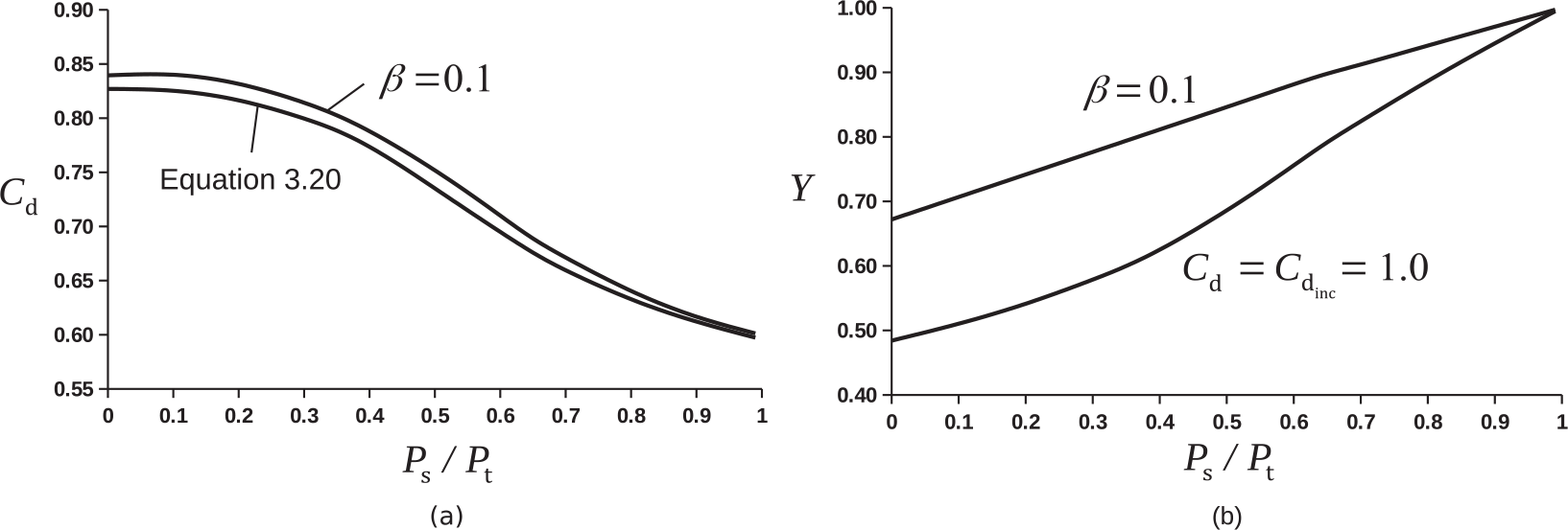
Figure 3.3 (a) Comparison of CdCd prediction by Equation 3.20 with the measurements of Perry (1949) for β = 0.1β=0.1 and (b) variation of adiabatic expansion factor Y with static-to-total pressure ratio.
A serious drawback of the method of computing CdCd using Equation 3.20 is that for β>0.5β>0.5 and low pressure ratios it yields Cd>1.0Cd>1.0, which is unacceptable. Parker and Kercher (1991) present a noniterative semi-empirical prediction method to generate intermediate values of CdCd between 0.5959 and 1.0 for 0.5959 ≤ Cdinc ≤ 1.00.5959≤Cdinc≤1.0 over the entire range of Ps/PtPs/Pt. The method, however, has limited experimental validation. High-fidelity CFD, including LES and DNS, may be used to generate CdCd for the entire range of orifice geometry and pressure ratio variations while validating these results against limited available experimental data.
3.1.2.2 Generalized Orifice
Figure 3.2b shows a generalized orifice featuring two geometric parameters, namely, the radius of curvature r/dr/d at the inlet and the length-to-diameter ratio L/dL/d and one inlet flow parameter representing the ratio of the tangential velocity to axial velocity Vθ/VxVθ/Vx. All three parameters, either individually or in combination, significantly affect the orifice discharge coefficient. The maximum benefit of the radius of curvature to minimize flow separation at the orifice inlet and the adverse effect of the vena contracta on discharge coefficient occurs at r/d≈1.0r/d≈1.0. For a thick orifice with L/d≈2L/d≈2, the sudden-expansion loss at the vena contracta is reduced, as a result, the discharge coefficient increases. For L/d>2L/d>2, the adverse affect of the orifice wall friction tends to decrease CdCd. The effect of Vθ/VxVθ/Vx is always to increase flow separation at the inlet causing deterioration in the orifice discharge coefficient. This can occur even with corner radiusing at the orifice inlet.
McGreehan and Schotsch (1988) present a design-friendly method to predict the effects of r/dr/d, L/dL/d and Vθ/VxVθ/Vx on discharge coefficient for a generalized orifice shown in Figure 3.2b. Their approach uses the classical adiabatic expansion factor to generate compressible flow discharge coefficient for a sharp-edged orifice. While the method shows good validation with the available test data for each individual parameter, its validation for the case featuring interaction effects of parameters is rather limited, and the method may at times predict Cd>1Cd>1. Parker and Kercher (1991) further improved the method of McGreehan and Schotsch (1988) by using the total-pressure mass flow function and ensuring that Cd ≤ 1Cd≤1 with a semi-empirical technique.
Existing methods of predicting orifice discharge coefficient for a rotating orifice are generally not reliable due a highly three-dimensional flow field caused by rotation within the orifice. These methods, therefore, tend to overpredict discharge coefficients for a rotating orifice. An obvious effect of rotation is to change Vθ/VxVθ/Vx at the orifice inlet. In addition, if the orifice inlet and outlet radii are appreciably different, the fluid total temperature relative to the orifice will change such that the rothalpy remains constant under adiabatic conditions. According to the isentropic relation, this change in fluid total temperature will results in a change in total pressure. Both these changes will affect the isentropic flow rate through the rotating orifice. Idris and Pullen (2005) present correlations to compute discharge coefficients for rotating orifices. A rotating long orifice with heat transfer and wall friction may alternatively be modeled as a duct, presented in Section 3.1.
From the foregoing discussion it is clear that the need for accurate and dependable 1-D modeling and prediction method for a general compressible flow orifice continues to exist. The lack of benchmark quality measurements in this area remains a serious impediment to further improvement – a situation that is not likely to change in the foreseeable future. Most of the available prediction methods are semi-empirical in nature with limited experimental validation. Another approach to mitigate the current situation is to leverage a CFD-based DOE using all key parameters that influence the discharge coefficient of a generalized orifice and correlating the results in the form a response surface. The response surface correlation can be easily implemented in a flow network code, which is used for modeling internal flow systems of modern gas turbines. The orifice response surface will predict both the direct and interaction effects of various parameters that influence the orifice discharge coefficient.
3.1.3 Vortex
The vortex is an important feature of a gas turbine internal flow system with rotor surfaces. In Chapter 2, we discussed isentropic free vortex, forced vortex, and nonisentropic generalized vortex and their modeling equations to compute pressure and temperature changes across them. The flow in a rotating duct creates a forced vortex that is coupled with other effects of friction and heat transfer. When an internal flow passes over rotor surfaces, like in rotor disk cavities, which we discuss in Chapter 4, it becomes a vortex with concurrent generation of windage.
It is important to note that, unlike a duct or an orifice, the vortex is not a physical component. It is simply a flow feature associated with its bulk circular motion (swirl) about the machine axis of rotation. Accordingly, unlike in a component, knowing the end conditions of a vortex, one may not be able to compute a unique mass flow rate associated with it. Therefore, a vortex will not qualify to be an element (discussed in the next section), which is directly connected to junctions in a flow network. We will henceforth call vortex a pseudo element. For its inclusion in a flow network, it must be sandwiched between two elements, either of which could be a duct or an orifice. The resulting super element, which becomes a mass flow metering component, can be connected to junctions in a flow network.
3.2 Description of a Flow Network: Elements and Junctions
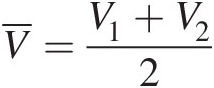
Gas turbine internal flow systems such as blade cooling system, rotor-stator or rotor-rotor cooling system, rotor-stator sealing system, discourager or rim seal system to minimize or prevent hot gas ingestion, inlet bleed heat system, and others are essentially handled using a flow network in which various components (ducts, orifices, seals, vortices, etc.) are modeled as 1-D flow element. Two basic entities of a flow network, shown in Figure 3.4, are element (also called link or branch) and junction (also called chamber or node). An element in this flow network is depicted by a solid line along with an arrow to represent the positive flow direction. A flow network has two types of junctions: internal junctions, depicted by an open circle, and the boundary junctions, depicted by an open square.
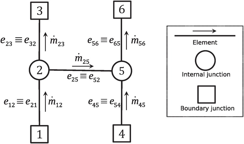
Figure 3.4 A flow network.
3.2.1 Element
An element of a flow network typically represents a component of the gas turbine internal flow system. A general flow network may include a variety of elements: duct, orifice, seal, vortex (pseudo component), heat exchanger (super element), and others. As shown in Figure 3.4, each element in the flow network connects two junctions. It is characterized by a mass flow rate, which in steady state remains constant from inlet to outlet. By its very function, an element in a network represents a flow metering device. The element connecting junctions ii and jj is represented by eijeij, which is the same as ejieji. Depending on the flow direction in the element, either of the junctions could be an inlet or an outlet. Note that the state variables at both junctions of an element uniquely determine the actual flow direction in the element. Later in this chapter, we will discuss a physics-based criterion to determine this flow direction. Even if one element in the network is assigned a wrong flow direction, the entire network solution is corrupted, which demonstrates the elliptic nature of the flow field modeled by a flow network, although a 1-D flow is assumed in each element.
Each element in a flow network is analogous to a thermodynamic path connecting two states of a system. All the path variables, evaluated in terms of the amount of work transfer and heat transfer, are associated with the flow through the element. In addition to the geometric parameters, empirical and semi-empirical correlations are specified for each element in the network to determine the friction factor for major loss, discharge coefficient for minor loss, and heat transfer coefficient to compute heat transfer in or out of the flow, etc. Various thermal and hydrodynamic boundary conditions applied to an element are assumed uniform; two- or three-dimensional variations of flow properties within the element are not discernible. These variations, if needed to develop a better understanding of the component, may be obtained through a CFD analysis, which may also be used readily to generate needed data to facilitate 1-D flow modeling of the component in the network to carry out a robust design.
At times, it becomes import to capture variations in geometry and boundary conditions over a flow element connecting two adjacent junctions. Examples include a long pipe line for bleed and coolant supply and the serpentine passage used for internal cooling of turbine airfoils. In such situations, the flow element may be modeled using serially-connected small control volumes without creating additional junctions in the overall network. This modeling practice offers significant economy in the network solution and preserves the dynamic pressure between adjacent control volumes in the flow direction for higher prediction accuracy.
There is often a debate among gas turbine engineers about which pressure, static or total, should be used at the junctions in a flow network to compute mass flow rate through the connecting elements. In steady state, the mass flow rate at any section in an internal flow requires that Pt>PsPt>Ps or Pt/Ps>1Pt/Ps>1, and this mass flow rate remains constant through the element or the gas turbine component that it represents, regardless of how fluid properties change from section to section. As discussed in Chapter 2, we can compute the element mass flow rate at any section using either the total-pressure mass flow function or the static-pressure mass flow function, both of which are functions of the section Mach number and the ratio of gas specific heats. This mass flow rate should be computed at the section, typically outlet, inlet, or where the flow is choked with M = 1M=1. This approach, however, doesn’t determine the flow direction across the section, which must be determined from the entropy change over the element.
It is important to note that the junction pressure at the inlet must be interpreted as the total pressure and that at the outlet as the static pressure. A junction with no associated dynamic pressure behaves like a plenum in which Pt = PsPt=Ps such that, for all flows leaving the junction, the plenum pressure becomes the total pressure, and for all flows entering the junction, the plenum pressure becomes the back pressure. For a subsonic flow through the element, the static pressure at the element exit section must equal the plenum back pressure (static). If, however, the flow is choked at the element exit, its static pressure becomes decoupled from the connected downstream junction, and the element mass flow rate is entirely determine by the upstream conditions. As an example, for the flow network shown in Figure 3.4, consider element e25e25 with the mass flow rate ṁ25 . Even in the presence of dynamic pressure at junction 2 due to the flow along e12e12 and e23e23, the total pressure at the inlet of element e25e25 equals the static pressure at junction 2. Similarly, for a subsonic flow through the element e25e25, its exit static pressure must be equal to the static pressure at junction 5.
3.2.2 Internal Junction
An internal junction connects two or more elements in a network. The flow network shown in Figure 3.4 has two internal junctions, namely, 2 and 5. The internal junction 2, for example, connects elements e12e12, e23e23, and e25e25. In steady state, the continuity equation for this junction yields
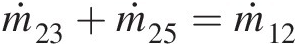 (3.22)
which, with ṁ21=−ṁ12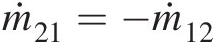 , can be written as
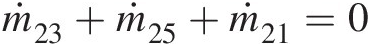 (3.23)
Thus, at an arbitrary internal junction ii connected through elements to multiple junctions j = 1j=1 to j = kij=ki, as shown in Figure 3.5, we can write the steady continuity equation as
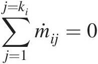 (3.24)
where j≠ij≠i. In this equation, we have adopted the convention that ṁij is nominally positive if the flow direction in the element eijeij is from junction ii to junction jj. According to this convention, we obtain ṁij=−ṁji
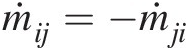 .
.
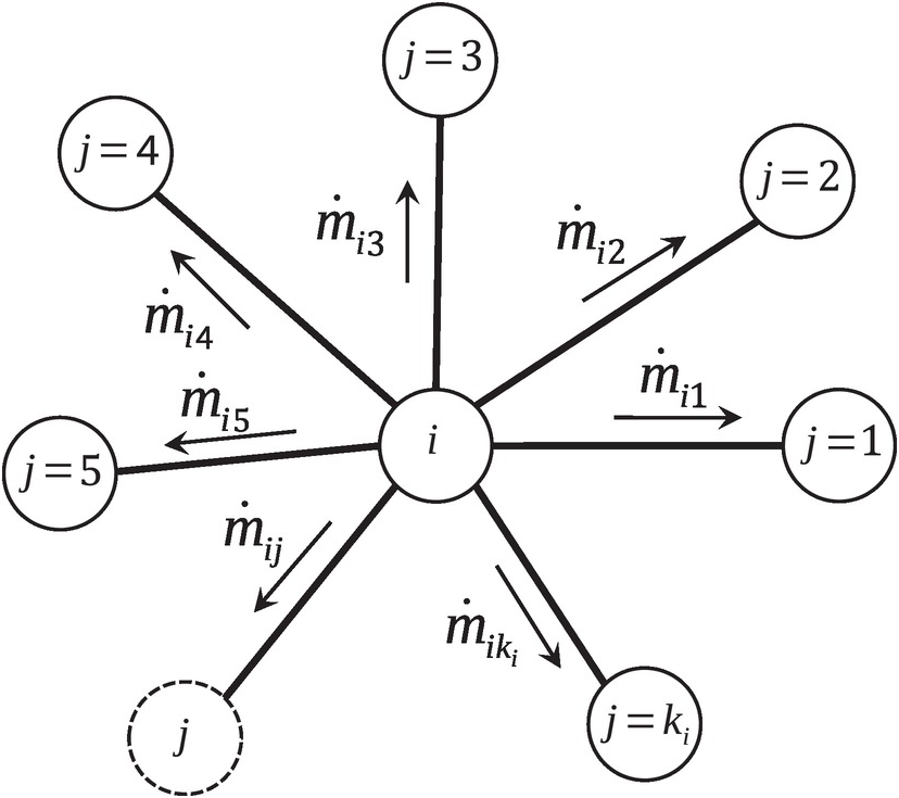
Figure 3.5 Mass conservation at an internal junction.
To ensure energy conservation at each internal junction, we can compute the mixed mean total temperature of all incoming flows. All outflows take place at this mixed mean total temperature. For example, we can write at junction ii
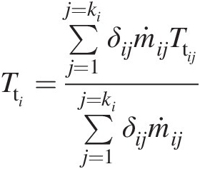 (3.25)
where we have δij = 1δij=1 for ṁij<0 (inflows) and δij = 0δij=0 for ṁij>0
 (outflows).
The foregoing discussion makes it clear that the net mass flow rate associated with an internal junction must be zero. All the state variables like pressure and temperature are associated with a junction. While the static pressure is uniform within a junction, the assumption of a uniform total pressure is a matter of modeling assumption depending upon the accuracy and rigor one needs in a design application. In this book, we limit our discussion to dump-type or plenum junctions, where we neglect the dynamic pressure associated with each incoming flow. This is akin to the “tank-and-tube” approach used in modeling a flow network. Sultanian (2015) presents more accurate and detailed modeling of junctions in a compressible flow network.
Thus, we model an internal junction with zero dynamic pressure in it, making the static and total pressures equal. In this case, the junction static temperature also equals the total temperature, which is determined by Equation 3.25 as the mixed mean total temperature of all flows entering the junction. All flows leaving the junction are assumed to be at this total temperature. By contrast, the static pressure of all subsonic flows entering the plenum junction equals the junction pressure, which becomes the total pressure for all flows leaving the junction.
3.2.3 Boundary Junction
A boundary junction in a flow network is either a source or a sink where the boundary conditions are specified. The network solution corresponds to these boundary conditions. Based on the flow directions shown in Figure 3.4, the boundary junctions 1 and 4 are the sources and the boundary junctions 3 and 6 are the sinks. Being sources and sinks, boundary junctions are allowed to violate the steady continuity equation. At a boundary junction, all state properties are generally assumed uniform.
3.3 Compressible Flow Network Solution
A flow network solution yields the mass flow rate through each element and the state properties, such as the total temperature and pressure, at each internal junction. Except for a very simple flow network, hand calculations to obtain a flow network solution could be very tedious and time-consuming. Therefore, the flow networks of gas turbine internal flow systems are typically solved using a computer with the help of a computer code based on a solution method similar to the one presented in this section. Because of nonlinear dependence of an element mass flow rate through on the difference in pressures at the connected junctions, a commonly used solution strategy is to iteratively perform the tasks of element solutions and junction solutions until the continuity equation at each internal junction is satisfied within an acceptable error.
In a flow network, for an assumed initial solution, all the mass flow rates generated in the connected elements will most likely not satisfy the continuity equation at each junction. The continuity Equation 3.24 becomes
 (3.26)
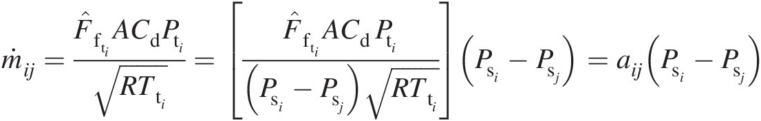
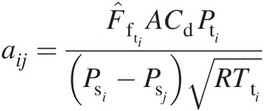
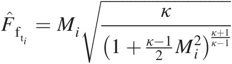
where Δṁi is the residual error in the continuity equation at junction ii. For the junction solution, let us assume that the mass flow rate ṁij
 through each element eijeij depends only on PsiPsi and PsjPsj. At each iteration, our goal is to change the junction static pressures so as to annihilate Δṁi
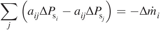
 in Equation 3.26. Accordingly, we can write
 (3.27)
Writing Equation 3.27 at each internal junction will result in a system of nonlinear algebraic equations for which no known direct solution method exists. One must therefore solve such a system using an iterative numerical method. At the current iteration, the system is treated as a linear system for which there are many numerical solution methods, for example, the direct method presented by Sultanian (1980); see also Appendix F.
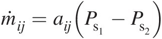
As shown in the foregoing discussion, we can express each element solution in the form ṁij=aijPsi−Psj , and assuming aijaij as constant at each iteration, we obtain ∂ṁij/∂Psi=aij
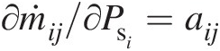 and ∂ṁij/∂Psj=−aij
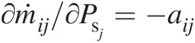 . Substituting them in Equation 3.27 yields
 (3.28)
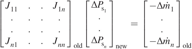
Writing Equation 3.28 for all internal junctions n in the flow network results in the following system of algebraic equations:
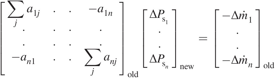 (3.29)
where the subscripts old and new refer to previous iteration and current iteration, respectively.
Note that the coefficient matrix aijaij, although assumed constant during the current iteration, varies from iteration to iteration until both the element and junction solutions are converged.
We can write Equation 3.29 in the following alternative form:
 (3.30)
where the coefficient matrix is known as the Jacobian matrix expressed as
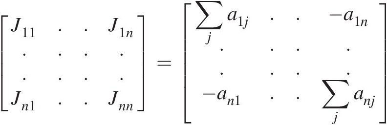 (3.31)
Because each junction in a typical flow network is connected to only a few neighboring junctions, the coefficient matrix in Equation 3.29 or the Jacobian in Equation 3.31 is generally very sparse with only a handful of nonzero entries.
3.3.1 Initial Solution Generation
An iterative solution method for a flow network requires an initial solution either as user input or generated automatically from the specified boundary conditions. For developing a robust design, which requires multiple probabilistic flow network solutions, it becomes imperative to eliminate any user intervention in obtaining each converged numerical solution.
For automatic generation of initial solution of the static pressure distribution at all internal junctions in a flow network, we can use one of the two methods. For the first method, we treat the flow network as a network of heat conduction rods each with the fixed thermal conductivity and geometry. The resulting system of equations will be linear for which we can directly solve for temperatures at all internal junctions. From the analogy between temperature and static pressure, we thus obtain the distribution of static pressure at all internal junctions of the flow network. For the second method, we use the fact that the relation between the pressure drop and mass flow rate in a fully developed laminar pipe flow is linear, given by the equation
 (3.32)
where
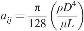
For the initial solution generation, we replace each element in the flow network by an equivalent laminar flow pipe. For the entire network, we will again obtain a system of linear equations that can be solved directly for static pressure at each internal junction.
3.3.2 Determination of Element Flow Direction
For a compressible flow network to yield accurate predictions, it is important that the flow direction in each element must be determined on physical grounds. We find that the entropy change over an element provides a sound physical basis to determine the element flow direction. For an adiabatic flow in an element when one or more effects of area change, friction, and rotation are present, the entropy must always increase in the flow direction. Accordingly, for the flow from section 1 to section 2 of such an element, we must have
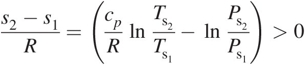 (3.33)
which involves static properties at these sections. In terms of total properties at these sections, we can write Equation 3.33 as
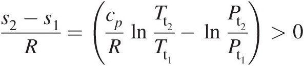 (3.34)
Based on the second law of thermodynamics, heat transfer always accompanies entropy transfer. Thus, heating of the element flow will increase its entropy downstream, and cooling will decrease it. Although heat transfer by itself is unlikely to change the flow direction in an element, for applying the entropy-based criterion, it is important to remove the contribution of heat transfer to the total entropy change over the element.
Equating the change in gas total temperature due to heat transfer across an element to the convective heat transfer through the element walls, we can write
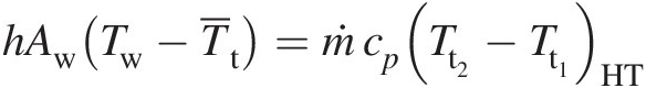
 (3.35)
According to Equation 3.35, the convective heat transfer in the element occurs at the average gas temperature T¯t . Thus, the entropy change due to heat transfer can be written as
 (3.36)
The positive value of the modified entropy change occurring in an element in the flow direction is given by
 (3.37)
which is the new criterion we can use to determine the flow direction in an element in the presence of heat transfer.
3.3.3 Newton-Raphson Method
Equation 3.29 represents the standard form used in the Newton-Raphson solution method, for example, presented by Carnahan, Luther, and Wilkes (1969) along with a computer program in FORTRAN.
The following key steps constitute the Newton-Raphson solution method:
1. Using one of the methods discussed in the foregoing, generate an initial distribution of static pressure at each internal junction of the flow network.
2. Compute mass flow rate through each element.
3. Compute Jacobian matrix from element solutions.
4. Compute mass flow rate error at each internal junction, yielding the right-hand side vector of Equation 3.29.
5. Use a direct solution method, for example Sultanian (1980), to obtain the vector of changes in static pressure at all internal junctions.
6. Obtain the new static pressure at each internal junction:
(Psi)new = (Psi)old + αi(ΔPsi)newPsinew=Psiold+αiΔPsinew
where αiαi is an under-relaxation parameter specified for each junction to help the solution convergence.
7. Repeat steps from 2 to 6 until Δṁimax≤δtol
 , where δtolδtol is the acceptable maximum error in the mass flow rate at an internal junction.
8. Solve the energy equation at each internal junction.
9. Repeat steps from 2 to 8 until (Tti)old−(Tti)newmax≤δ̂tol
 , where δ̂tol
 is the maximum acceptable difference between the total temperatures at any internal junction in successive iterations.


The standard Newton-Raphson method outlined earlier has two main shortcomings. First, the solution convergence is found sensitive to the initial solution assumed for the network. Second, when using a computer code to perform the computations, the user-specified under-relation parameters may need adjustments when the network solution starts diverging. In an integrated design environment, when a designer is required to generate multiple solutions of a flow network for a probabilistic (robust) design, these shortcomings of the solution method may become a serious handicap. The modified Newton-Raphson method presented in the next section provides a robust solution methodology, ideally suited for a complex compressible flow network used in gas turbine design.
3.3.4 Modified Newton-Raphson Method
In the modified Newton-Raphson method, a positive damping parameter λλ is added to each diagonal element of the Jacobian matrix. Equation (3.30) now becomes
 (3.38)
where the damping parameter λλ, which is auto-adjusted during the iterative solution process, ensures that the Jacobian matrix remains diagonally dominant, preventing it from becoming singular. In this form, the modified Newton-Raphson method is equivalent to the linear least-squares optimization based on Levenberg-Marquardt method presented in Nash and Sofer (1996). This modified Newton-Raphson solution method consists of the following key steps:
1. Using one of the methods discussed in the foregoing, generate an initial distribution of static pressure at each internal junction of the flow network.
2. Set λold = 0.5λold=0.5 and λnew = λoldλnew=λold.
3. Compute mass flow rate through each element.
4. Compute residual error of the continuity equation at each internal junction and the corresponding error norm
Eold=1n∑i=1nΔṁi2
5. Compute Jacobian matrix from solution for each element in the flow network.
6. Modify the Jacobian matrix by adding λnewλnew to all its diagonal components.
7. Use a direct solution method, for example, Sultanian (1980), to obtain the vector of changes in static pressure at all internal junctions.
8. Obtain the new static pressure at each internal junction:
(Psi)new = (Psi)old + (ΔPsi)newPsinew=Psiold+ΔPsinew
9. Compute mass flow rate through each element.
10. Compute error of the continuity equation at each internal junction and the error norm
Enew=1n∑i=1nΔṁi2
11. If Enew>EoldEnew>Eold, set λnew = 2λoldλnew=2λold and repeat steps from 6 to 11.
12. Set λnew = λold/2λnew=λold/2
13. Repeat steps from 5 to 12 until Enew≤δ˜tol
 , where δ˜tol
 is the acceptable maximum value of EnewEnew
14. Solve the energy equation at each internal junction.
15. Repeat steps from 5 to 14 until Ttiold−Ttinewmax≤δ̂tol
 , where δ̂tol
 is the maximum acceptable difference between the total temperatures at any internal junction in successive iterations.


3.4 Concluding Remarks
Physics-based 1-D flow modeling of each component of a gas turbine internal flow system satisfies the conservation equations of mass, momentum, energy, and entropy, which provides a robust criterion to determine the flow direction in the flow. Any elliptic flow feature involving flow separation and reversal within the component is accounted for using empirical correlations to compute pressure loss and heat transfer coefficient. Understanding of these flow features in a component may be discerned from a three-dimensional CFD analysis, reinforcing an improved 1-D flow modeling of the component.
Because the internal flow system boundary conditions are generally known only at the source (gas turbine main flow path) and sink (ambient or downstream gas turbine flow path), intermediate flow properties are obtained from the solution of a flow network. In this network, each element, whose mass flow rate is a single-valued function of the properties at the connected end junctions, represents a system component. Because a unique mass flow rate cannot be obtained from the property changes across a vortex, it does not qualify to be an element of the flow network. It is therefore named here a pseudo element and must be sandwiched between two elements for its integration into the flow network.
The compressible flow network formulations presented in this chapter have no Mach number limitation. In addition to the effects of area-change, friction, and heat transfer, the formulation also includes the effects of rotation in each element. For the development of a computer code to handle a flow network, we have discussed here key details of the physics-based modeling methods for elements and junctions that form the network. We have also presented here a modified Newton-Raphson method for the robust iterative numerical solution of a system of nonlinear algebraic equations, which generally arise from the flow network modeling of a gas turbine internal flow system.
Worked Examples
Example 3.1
Consider an orifice with diameter D = 30 mmD=30mm, upstream total pressure Pt1 = 12 barPt1=12bar, constant total temperature Tt1 = 781 KTt1=781K, and downstream static pressure Ps2 = 10 barPs2=10bar. Assume the orifice discharge coefficient Cd = 0.8Cd=0.8 for the following:
(1) Compute air mass flow rate through the orifice
(2) Compute the total pressure (Pt2Pt2) at the orifice exit
(3) Defining the orifice loss coefficient K = (Pt1 − Pt2)/(Pt2 − Ps2)K=Pt1−Pt2/Pt2−Ps2 and using the relation Cd=1/K+1
 derived in Chapter 2, compute the orifice exit total pressure and find the percentage error from its value computed in (2)
Solution
Duct flow area: A=πD24=π×0.03024=0.707×10⁻³m2
Loss coefficient: From Cd=1/K+1 , we can write
(1) Mass flow rate through the orifice
Pt1Ps2=12×10510×105=1.2
Tt1Ts2=Pt1Ps2κ−1κ=1.20.286=1.0535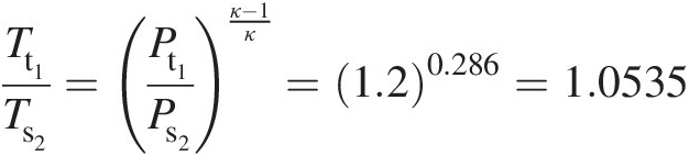
M1=2κ−1×Tt1Ts2−1=5×1.0535−1=0.517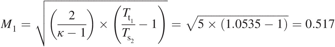
F̂ft1=M1κ1+κ−12M12κ+1κ−1=0.517×1.41.05356=0.5233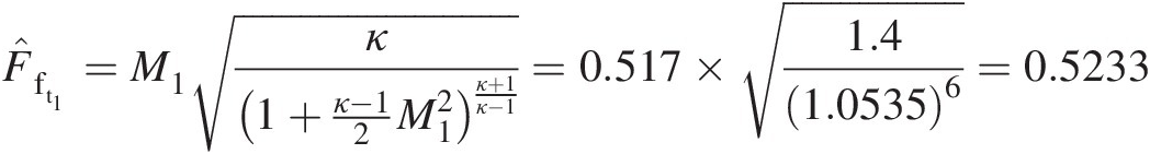
ṁ=CdAF̂ft1Pt1RTt1=0.8×0.707×10−3×0.5233×12×105287×781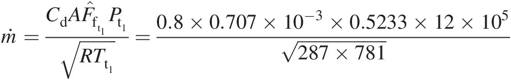
ṁ=0.750kg/s
(2) Total pressure at orifice exit (section 2)
We can write the mass flow rate in terms of static-pressure mass flow function at orifice exit (section 2) as
ṁ=AF̂fs2Ps2RTt1which yields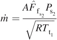
F̂fs2=ṁRTt1APs2=0.750×287×7810.707×10−3×10×105=0.5024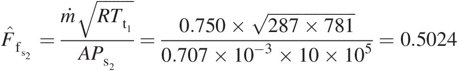
Using Equation 2.106, we obtain the Mach number at orifice exit (section 2) as
M2=−κ+κ2+2κκ−1F̂fs22κκ−1=−1.4+1.42+2×1.4×1.4−1×0.502421.4×1.4−1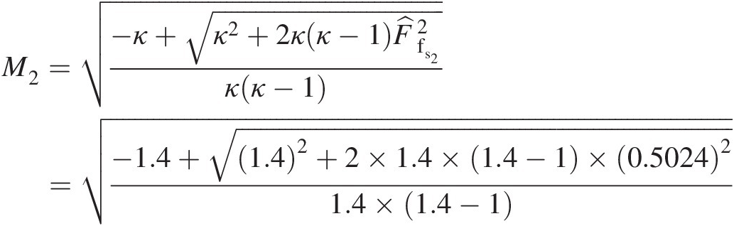
Using isentropic relations, we obtain
M2 = 0.4174M2=0.4174
Pt2Ps2=1+κ−12M2κκ−1=1+1.4−120.417423.5=1.1273which yields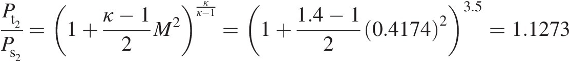
Pt2 = 1.1273 × Ps2 = 1.1273 × 10 × 105Pt2=1.1273×Ps2=1.1273×10×105
Pt2 = 11.273 × 10⁵ PaPt2=11.273×10⁵Pa
(3) Total pressure at orifice exit using the loss coefficient K = (Pt1 − Pt2)/(Pt2 − Ps2)K=Pt1−Pt2/Pt2−Ps2
We rearrange the given definition for the loss coefficient K = (Pt1 − Pt2)/(Pt2 − Ps2)K=Pt1−Pt2/Pt2−Ps2 to compute the orifice exit total pressure as
Pt2=Pt1+KPs21+K=12×105+0.563×10×1051+0.563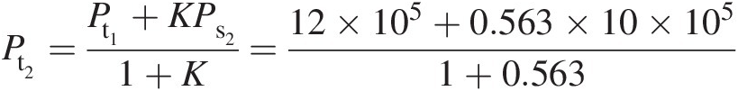
Pt2 = 11.280 × 10⁵ PaPt2=11.280×10⁵Pa


which is within an acceptable error of 0.0587 percent from the value computed in (2) using the static-pressure mass flow function computed at the orifice exit with the specified static pressure.
Example 3.2
Cooling air flows through a circular duct of diameter 0.025 m0.025m and length 1.0 m1.0m at inlet conditions of Pt1 = 1.5 barPt1=1.5bar and Tt1 = 573 KTt1=573K. The duct wall temperature remains uniform at 1023 K1023K. Divide the duct in ten equal segments. For the air mass flow rate of 0.1 kg/s0.1kg/s through the duct, compute the following for the first duct segment of length 0.1 m0.1m:
1. At section 1 (duct inlet): Mach number (M1M1), static pressure (Ps1Ps1), and static temperature (Ts1Ts1)
2. At section 2 (exit of the first duct segment): Mach number (M2M2), static pressure (Ps2Ps2), static temperature (Ts2Ts2), total pressure (Pt2Pt2), and total temperature (Tt2Tt2)
3. Change in entropy. Verify that the criterion for determining the flow direction in the duct is satisfied.
For the computations, assume the following air properties and empirical correlations:
Air properties: κ = 1.4κ=1.4; R = 287 J/(kg K)R=287J/kgK; k = 0.0429 W/(m K)k=0.0429W/mK; Pr = 0.71Pr=0.71
Empirical equation to compute friction factor: f=11.82log10Re−1.642
Empirical equation to compute heat transfer coefficient (Dittus-Boelter equation):
Nu=0.023Re0.8Pr0.334orh=0.023kDRe0.8Pr0.334
Solution
In this example, the cooling air flow through the duct is subjected to both friction and heat transfer. The solution method presented here, however, can be easily extended to include change in duct flow area and duct rotation about an axis other than its own axis; see Problem 3.5.
Some Preliminary Calculations:


Duct flow area: A=πD24=π×0.02524=0.491×10⁻³m2
Duct surface area for heat transfer: Aw = πDL = π × 0.025 × 0.1 = 7.854 × 10⁻³ m2Aw=πDL=π×0.025×0.1=7.854×10⁻³m2
1. Quantities at section 1 (duct inlet)
Total-pressure mass flow function: F̂ftin=ṁRTt1APt1=0.1287×5730.491×10−3×1.5×105=0.551
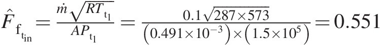
Using an iterative solution method, for example, “Goal Seek” in EXCEL, we obtain M1 = 0.553M1=0.553.
From isentropic relations we obtain
Ts1=Tt11+1+κ2M12=5731+0.51+1.40.5532=539.9K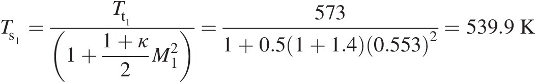
Ps1=Pt1Ts1Tt1κκ−1=1.5×105539.95733.5=121831Pa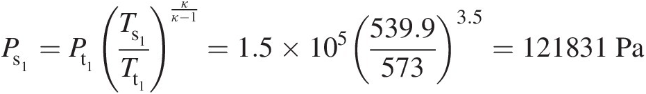
Inlet velocity: V1=M1κRTs1=0.553×1.4×287×539.9=257.717m/s

Therefore, at section 1 (duct inlet), we obtain M1 = 0.553M1=0.553, Ts1 = 539.9 KTs1=539.9K, and Ps1 = 121831 PaPs1=121831Pa.
2. Quantities at section 2
Let us first calculate the total temperature Tt2Tt2 as follows:
Reynolds number: Re=ρVDμ=ρVADμA=ṁDμA=0.1×0.0253.0323×10−5×0.491×10−3

Re = 1.68 × 10⁵Re=1.68×10⁵
Nusselt number: Nu = 0.023Re0.8Pr0.334 = 0.023 × (1.68 × 105)0.8 × (0.71)0.334 = 310.61Nu=0.023Re0.8Pr0.334=0.023×1.68×1050.8×0.710.334=310.61
Heat transfer coefficient: h=kDNu=0.04290.025×310.61=533Wm2K

Number of transfer units (NTU):
η=Awhṁcp=7.854×10−3×5330.1×1004.5=4.167×10⁻²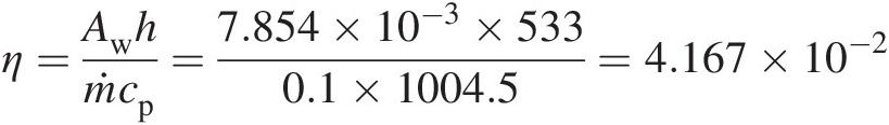


Using Equation 3.12, we compute the air total temperature at section 2 as
To compute remaining quantities at the duct outlet, we present in the following an iterative solution method. The converged value of each quantity is given within parentheses.
Step 1: Assume M2M2 (M2 = 0.593M2=0.593)
Step 2: Compute F̂ft2
 : F̂ft2=Mκ1+κ−12M22κ+1κ−1
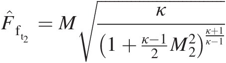 (F̂ft2=0.572)
Step 3: Compute Pt2Pt2: Pt2=ṁRTt2AF̂ft2
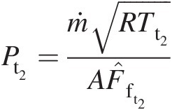 Pt2 = 146706 Pa(Pt2=146706Pa)
Step 4: Compute Ts2Ts2: Ts2=Tt21+1+κ2M22
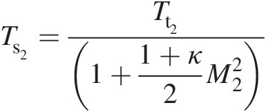 Ts2 = 552.5 K(Ts2=552.5K)
Step 5: Compute Ps2Ps2: Ps2=Pt2Ts2Tt2κκ−1
 Ps2 = 115670 Pa(Ps2=115670Pa)
Step 6: Compute V2V2: V2=M2κRTs2
 (V2 = 279.29 m/sV2=279.29m/s)
Step 7: Compute ΔPsfΔPsf: ΔPsf=f2LDṁAV1+V22
 ΔPsf = 1766 Pa(ΔPsf=1766Pa)
Step 8: Compute P̂s2
 from the force-momentum balance on the duct control volume using
P̂s2=Ps1−ΔPsf−ṁAV2−V1(P̂s2=115670Pa)
Step 9: Repeat Steps 1 to 8 until Ps2Ps2 computed in Step 5 is within an acceptable difference with P̂s2
 computed in Step 8.


The required quantities computed at section 2 are summarized as follows:
3. Entropy change between sections 1 and 2:
s2−s1R=cpRlnTt2Tt1−lnPt2Pt1=1004.5287ln591.4573−ln146706150000=0.1326
For the entropy-based criterion for determining the flow direction in an element in the presence of heat transfer, we need to use Equation 3.37 for which the average gas total temperature for heat transfer is first computed as
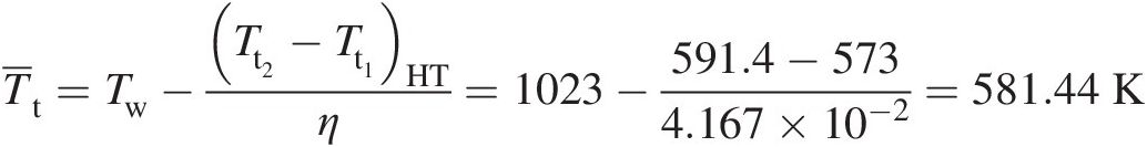
Then, Equation 3.36 yields
Finally, using Equation 3.37 we obtain

which is positive, satisfying the criterion for the element flow direction from section 1 to section 2.
Example 3.3
Consider a Fanno flow in a pipe of 0.0508 m0.0508m diameter and average Darcy friction factor of 0.022. The total pressure and temperature at the pipe inlet are 11 bar11bar and 459 K459K, respectively. Assuming κ = 1.4κ=1.4 and R = 287 J/(kg K)R=287J/kgK for air, calculate the maximum pipe length to deliver a mass flow rate of 1.75 kg/s1.75kg/s for both subsonic and supersonic inlet conditions. In each case, determine the total pressure at the pipe exit.
Solution
In this example, for the given total pressure and total temperature at the pipe inlet, both subsonic and supersonic flow solutions are possible for the specified mass flow rate through the pipe. In both cases, the flow chokes at the pipe exit (Mexit = 1Mexit=1), albeit requiring different pipe lengths.
(a) Subsonic flow at inlet
Pipe flow area: A=πD24=π×0.050824=2.027×10⁻³m2
Inlet Mach number: We can compute the mass flow rate at pipe inlet by the equation

where F̂fta is the total-pressure mass flow function for case (a), and it is given by the equation
which; upon using, for example, the “Goal Seek” function in Excel with a subsonic Mach number as the initial guess, yields Minlet(a) = 0.25Minleta=0.25.
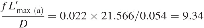
Maximum pipe length: Using the inlet Mach number, we compute f Lmax(a)/DfLmaxa/D by the Fanno flow equation from Table 2.4, we obtain

which gives
Total pressure at pipe exit: Using the Fanno flow equation in Table 2.4, we compute the inlet-to-exit total pressure ratio as

which yields

(b) Supersonic flow at inlet
Inlet Mach number: We again use an iterative method (e.g., the “Goal Seek” function in Excel with a supersonic Mach number as the initial guess) to solve the following equations

and
and obtain Minlet(b) = 2.4Minletb=2.4.
Maximum pipe length: Using Minlet(b) = 2.4Minletb=2.4, we compute f Lmax(a)/DfLmaxa/D by the Fanno flow equation from Table 2.4 as

which gives

Total pressure at pipe exit: Using the Fanno flow equation in Table 2.4, we compute

which yields
The results obtained in this example indicate that the maximum pipe length with subsonic inlet is 19.606 m19.606m and that with supersonic inlet 0.947 m0.947m, which provides a much shorter delivery system. For creating a subsonic inlet flow, we can use an isentropic convergent nozzle; for creating a supersonic inlet flow, we can use an isentropic convergent-divergent nozzle. In the latter case, however, the flow system will have two sonic sections, one at the physical throat of the nozzle and the other at the pipe exit.
The fact that in both cases we obtain the same total pressure at the pipe exit should not be surprising. For both subsonic-inlet and supersonic-inlet cases, we have at the pipe inlet identical total pressure, total temperature, and mass flow rate, which remains constant throughout the pipe. At the pipe exit, the flow is choked with Mexit = 1Mexit=1, yielding a constant value of total-pressure mass flow function (Fft∗=0.6847 ). Because the total temperature remains constant in a Fanno flow, the mass flow rate equation should yield the same value for the exit total pressure for both cases. Also, from isentropic relations, we can conclude that the static pressure at the pipe exit should also be identical for both cases. Because the frictional pressure loss per unit length of the pipe for the supersonic flow will be much higher, due to its higher velocities, than for the subsonic flow, we obtain a much shorter length for the same overall loss in total pressure and change in static pressure over the pipe from its inlet to exit.
Example 3.4
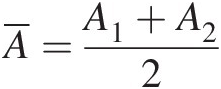
Reconsider the Fanno flow of Example 3.3. Without changing the specified total pressure and temperature at the pipe inlet, calculate and describe the properties of the new Fanno flow of air if the maximum pipe lengths with sonic exit computed for the subsonic and supersonic inlet conditions are extended by10 percent. In both cases, shown in Figure 3.6, the flow remains choked at the extended pipe exit.

Figure 3.6 (a) Pipe extension in an initially choked Fanno flow with subsonic inlet and (b) pipe extension in an initially choked Fanno flow with supersonic inlet (Example 3.4).
Solution
Figure 3.6 schematically (not to scale) shows pipe extensions in initially choked Fanno flows with subsonic and supersonic inlet conditions. As shown in Figure 3.6(a), when we extend a choked Fanno flow with a subsonic inlet, the sonic section moves downstream to the extended pipe exit with reduction in both mass flow rate and exit total pressure. A choked Fanno flow with a supersonic inlet, shown in Figure 3.6(b), features a different flow behavior when the pipe is extended beyond its maximum length. Because the downstream changes are not communicated upstream in a supersonic flow, the pipe extension results in a normal shock at an intermediate section. The supersonic flow upstream of the normal shock becomes subsonic downstream and reaches the sonic condition at the extended pipe exit. In this case, interestingly, the mass flow rate and total pressure at the new exit remain unchanged.
(a) Subsonic flow at inlet
With reference to Figure 3.6(a), the inlet conditions and calculated properties from Example 3.3 are summarized here:
With 10 percent extension of the pipe, the new maximum pipe length becomes

which yields
Using the “Goal Seek” iterative solution method in Excel, we obtain the new inlet Mach number from the equation in Table 2.4 as Minleta′=0.241 . With this value of inlet Mach number, we calculate the new mass flow rate as ṁa′=1.689kg/s
 , which is 3.51%3.51% lower than the initial value of 1.75 kg/s1.75kg/s without the pipe extension. Similarly, at Minleta′=0.241
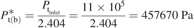
 , we compute the new exit total pressure as P′texita∗=441616Pa
 , which is also 3.51%3.51% lower than its value calculated in Example 3.3.
(b) Supersonic flow at inlet
With reference to Figure 3.6(b), the inlet conditions and calculated properties from Example 3.3 are summarized here:
With 10 percent extension of the pipe, the new maximum pipe length becomes

From the flow physics presented earlier for this case, it is clear that the conditions at the pipe inlet and new exit remain the same as before the pipe is extended. We only need to find the distance LNSLNS from the pipe inlet where the normal shock occurs. From Figure 3.6(b), we can write
and
where
Lmax(b)≡Lmaxb≡ Maximum pipe length that corresponds to the supersonic Mach number at the pipe inlet
Lmax1(b)≡Lmax1b≡ Maximum pipe length computed at M1M1
Lmax2(b)≡Lmax2b≡ Maximum pipe length computed at M2M2.
Note that M1M1 is the supersonic Mach number upstream of the normal shock, and M2M2 is the corresponding downstream subsonic Mach number.
We present next the steps of an iterative solution method to calculate LNSLNS.
1. Assume M1M1.
2. Calculate M2M2 with the following normal shock equation in Table 2.6:
M22=κ−1M12+22κM12−κ−1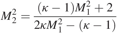
3. Calculate f Lmax1(b)/DfLmax1b/D at M1M1, hence Lmax1(b)Lmax1b.
4. Calculate LNS = Lmax(b) − Lmax1 (b)LNS=Lmaxb−Lmax1b.
5. Calculate f Lmax2(b)/DfLmax2b/D at M2M2, hence Lmax2(b)Lmax2b.
6. Repeat steps from 1 to 6 until Lmaxb′=LNS+Lmax2b
 .
.

Using “Goal Seek” in Excel, the aforementioned iterative method yields the following values for various quantities.
When the initially choked pipe flow with the supersonic inlet is extended, the aforementioned results show that the normal shock within the pipe converts the upstream supersonic flow into a subsonic flow downstream, keeping the loss in total pressure from pipe inlet to exit constant. This feature of a choked supersonic Fanno flow makes it an ideal constant mass flow delivery system that is robust to variations in downstream conditions.
Problems
3.1 Consider the orifice of Example 3.1 under adiabatic compressible flow. Six of such orifices are connected in series. The inlet boundary conditions for this arrangement are the same as given for the single orifice in Example 3.1. The fixed static pressure at the exit of the sixth orifice is 10 bar10bar. This flow network has five internal nodes and two boundary nodes, where the required boundary conditions are known. The flow being adiabatic, the total temperature remains constant throughout the network.
(1) Assuming total loss of the dynamic pressure at the exit of each orifice, sequentially carry out the solution for each orifice to determine the network mass flow rate, including the static and total pressure at each internal node. You may have to repeat this a few times with an initial guess for the mass flow rate to ensure that the computed exit static pressure equals the specified value.
(2) Repeat the calculations of (1) to find the minimum total pressure at inlet needed to achieve the choked flow condition in the orifice network. Where does the flow choke? What is the resulting network mass flow rate in this case?
(3) Find the network mass flow rate if the inlet total pressure is 10 percent higher than the minimum inlet total pressure for choking computed in (2).
Carry out solutions of (1), (2), and (3) using the following alternate approach. For the compressible flow through an orifice whose upstream end is connected to node ii and the downstream end connected to node jj, we can express the mass flow rate as
where
Note that the coefficient aijaij is not a constant, giving a nonlinear relation between the mass flow rate and difference in static pressures across the orifice. Although we have assumed a constant value for the discharge coefficient CdCd in this problem, experimental measurements suggest that it is a function of the pressure ratio across the orifice.
Writing the aforementioned equation for the mass flow rate through each orifice in the series network and noting that, at each internal node, the mass flow rate of the upstream orifice equals that of the downstream orifice, leads a simultaneous system of equations for the unknown nodal pressures where the coefficient matrix in tridiagonal. Such a system of equations is easily solved using the tridiagonal matrix algorithm, a FORTRAN routine for which is listed in Appendix E. In this approach, however, we need an initial guess for the internal nodal pressures. In addition, because the coefficients are solution-dependent, we need to iterate them to reach convergence.
Compare the results obtained using both approaches and comment on their relative advantages and disadvantages.
3.2 Verify the solution presented for Example 3.2 for the first duct segment of length 0.1 m. Repeat the solution sequentially for the remaining duct segments to compute the duct outlet conditions. Do these results change significantly if you divide the duct into 20 and 40 segments?
3.3 Having developed the numerical solution method in Problem 3.2, it is important to compare its computed results against the known exact solutions for Fanno and Rayleigh flows. For the Fanno flow, set Tw = TtTw=Tt in each pipe segment to achieve zero heat transfer. Although physically unrealistic, you may also artificially set h = 0h=0 to achieve an adiabatic pipe flow. Compare your results at the pipe outlet with the results obtained using the Fanno flow equations presented in Chapter 2. For the Rayleigh flow, set pipe friction factor f = 0f=0 in your solution method and compare the results at the pipe outlet with the results obtained using the Rayleigh flow equations presented in Chapter 2. Note that achieving a good comparison with the exact Fanno and Rayleigh flow solutions is a necessary condition, but it does not constitute the sufficient validation of the numerical solution method, which computes the combined effects of friction and heat transfer on the duct flow.
3.4 Repeat Example 3.2 for the case of a variable-area duct. First, consider a linearly converging duct with inlet-to-outlet area ratio of 2. Second, consider a linearly diverging duct of outlet-to-inlet area ratio of 2.0.
3.5 Consider the design situation where the variable-area duct used in Problem 3.4 is rotating at an angular velocity Ω = 300 rad/sΩ=300rad/s. The angle between the duct axis and the axis of rotation is 60°60°. Including the effects of duct rotation, repeat your calculations in Problem 3.4 for both converging and diverging ducts.
3.6 The numerical solution method developed Problem 3.5 allows one to simulate air flow in a variable-area duct under the coupled influence of friction, heat transfer, and rotation. Using this solution method, one can also obtain the solution with each effect separately or for various combinations of these effects. For the same inlet conditions of total pressure, total temperature and mass flow rate, obtain solutions for pressure and temperature variation throughout the duct for each individual effect of area change, friction, heat transfer, and rotation. Over each duct segment, add the changes in static pressure due to each effect of area change, friction, heat transfer, and rotation and compare the resulting variation in static pressure over the duct with that obtained in Problem 3.5. Again, over each duct segment, add the changes in total pressure due to each effect of area change, friction, heat transfer, and rotation and compare the resulting variation in total pressure over the duct with that obtained in Problem 3.5. Comment on your results of comparison.
3.7 In Problem 3.5, numerical results are obtained for the specified inlet boundary conditions of total pressure, total temperature, and mass flow rate. In most design applications, and in a flow network solution, we need to compute the mass flow rate through the duct under the boundary conditions of total pressure and temperature at its inlet and static pressure at its outlet. For an outlet pressure of 1 bar1bar, modify the numerical method used in Problem 3.5 to compute the resulting mass flow rate through the duct under the specified inlet total pressure and total temperature. At what inlet total pressure will the flow choke in the duct? Find the corresponding mass flow rate and the location of choking (M = 1M=1).
3.8 Divide the duct of Example 3.2 into 40 equal segments and carry out the numerical solution under adiabatic conditions with wall friction only, which corresponds to a Fanno flow. Representing each duct segment as an orifice with its mechanical area equal to the duct area and its pressure and temperature conditions from the numerical Fanno flow solution, find the variation in orifice discharge coefficient along the duct from inlet to outlet.

Figure 3.7 Serially-coupled isentropic and nonisentropic compressible flows (Problem 3.10).
3.9 In a flow network, when orifices are connected in series, it is generally assumed that the dynamic pressure from the upstream orifice is lost in the junction connecting two orifices. In Problem 3.8, we simulated a Fanno flow using orifices in series, one orifice for each duct segment, without losing the interorifice dynamic pressure. Repeat the calculations to determine the discharge coefficient of each orifice under the assumption that the static pressure downstream of each orifice (duct segment) becomes the total inlet pressure of the next orifice. Compare the variation in orifice discharge coefficients along the duct with that obtained in Problem 3.8.
3.10 The diagram here shows an air flow system consisting of an isentropic flow through a convergent-divergent (C-D) nozzle with exit diameter of 0.1 m, a Fanno flow, and 0.5 m long Rayleigh flow. The pipe diameter of both the Fanno flow and the Rayleigh flow equals the exit diameter of the C-D nozzle. Without the 0.5 m pipe extension (Rayleigh flow), the flow system remains free from any normal shock, and delivers the required mass flow rate of 1.0 kg / s with Mexit = 1Mexit=1 at the end of the Fanno flow when the inlet total pressure and total temperature are 16.5 bar and 1000 K, respectively. With the 0.5 m pipe extension (Rayleigh flow), which is needed to further increase the air total temperature by 100 K through uniform heating, the flow undergoes a normal shock somewhere between the C-D nozzle throat and the end of the Rayleigh flow where Mexit = 1Mexit=1 with the same inlet total pressure and total temperature of 16.5 bar and 1000 K, respectively.
Assumptions and data:
1. The compressible air flow is one-dimensional and air is considered a calorically perfect gas having the equation of state: Ps = ρsRTsPs=ρsRTs, where R = 287 J/(kg K)R=287J/kgK.
2. Ratio of air specific heats: κ = cp/cv = 1.4κ=cp/cv=1.4.
3. In the divergent section of the C-D nozzle, the diameter varies linearly from throat to nozzle exit.
4. The normal shock has zero thickness.
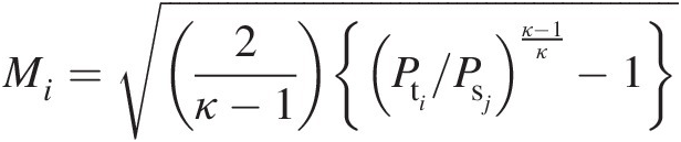
3.11 Figure 3.8 shows a pipe of diameter D = 50 mmD=50mm with six equispaced converging nozzles, which are to be sized to yield equal mass flow rate of hot air through them to promote uniform mixing with a large cross flow. The hot air enters the mixing arm at the total pressure and temperature of 1.1 bar1.1bar and 1000 K1000K, respectively. All converging nozzles discharge into the cross flow at a static pressure of 1.0 bar1.0bar. Assume that the flow is adiabatic in the entire mixing arm with constant Darcy fiction factor f = 0.02f=0.02 in the main pipe. Furthermore, assume that the flow is isentropic in each nozzle.
(a) Setting each nozzle exit area equal to one-sixth of the pipe flow area, find the mass flow rate through each nozzle.
(b) Adjust the nozzle jet area to ensure equal mass flow rate through each nozzle. What is the total mass flow rate through the mixing arm? What is the exit area of each nozzle?
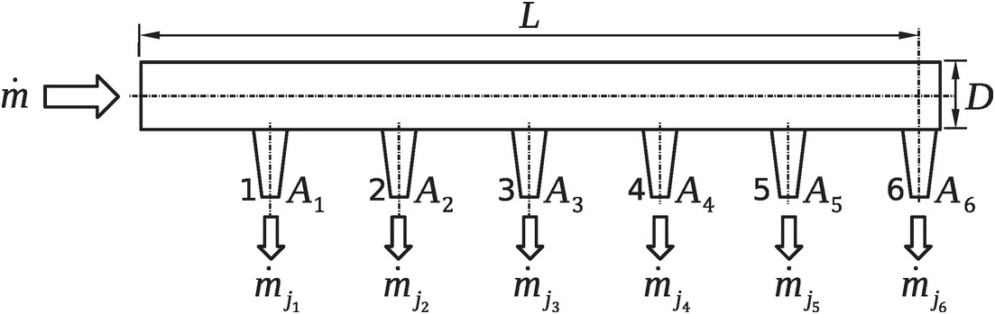
Figure 3.8 A low-pressure uniform mixing arm with converging nozzles (Problem 3.11).
3.12 Figure 3.9 shows a pipe of diameter D = 50 mmD=50mm with six equispaced converging-diverging (C-D) nozzles, which are to be sized to yield equal mass flow rate and jet velocity of cold air for impingement cooling of a hot surface. The high-pressure cold air enters the impingement arm at the total pressure and temperature of 11 bar11bar and 500 K500K, respectively. All converging-diverging nozzles discharge the coolant air on a surface maintained at a uniform static pressure of 1.5 bar1.5bar. Assume that the flow is adiabatic in the entire impingement arm with constant Darcy fiction factor f = 0.02f=0.02 in the main pipe. Furthermore, assume that the flow is isentropic in each nozzle.
(a) Determine the total mass flow rate at the pipe inlet and critical throat area of each C-D nozzle to deliver one-sixth of this flow rate.
(b) Determine each nozzle exit area so that the impingement jet velocities of all nozzles are equal.
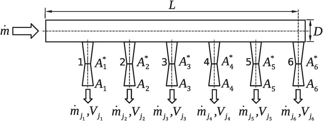
Figure 3.9 A high-pressure jet impingement cooling arm with converging-diverging nozzles (Problem 3.12).
3.13 Repeat the solution of Example 3.1 for four values of the discharge coefficient CdCd, namely, 0.6, 0.7, 0.8, and 0.9, and, for each value, use four values of the orifice inlet total pressure Pt1Pt1, namely, 11 bar, 13 bar, 15 bar, and 17 bar, keeping all other given data unchanged. Based on your calculation results, will you recommend in a design application the method of calculating the orifice exit total pressure using the loss coefficient K?
3.14 Repeat the solution of Example 3.1 with the orifice inlet total pressure Pt1 = 20 barPt1=20bar, keeping all other given data unchanged. Note that the pressure ratio across the orifice in this case will exceed the critical pressure ratio for a choked flow condition. Comment on the validity of calculating the orifice exit total pressure using the loss coefficient K?
3.15 Solve Example 3.3 by discretizing the duct into small segments and using the numerical method used in Example 3.2 for the solution over a duct segment.
3.16 Solve Example 3.4 by discretizing the duct into small segments and using the numerical method used in Example 3.2 for the solution over a duct segment.
Project
3.1 Develop a stand-alone, general purpose computer code in FORTRAN, or the language of your choice, to solve for the properties of 1-D compressible flow in a variable-area duct under the coupled effects of friction, heat transfer, and duct rotation about an axis inclined to the duct axis. The code should work at all Mach numbers corresponding to subsonic, sonic (internal choking), and supersonic flow regimes, including the possibility of a normal shock, which is the nonisentropic mechanism a supersonic flow uses to abruptly become subsonic. How will you verify your computer code, and how will you validate it?
References
Bibliography
Nomenclature
- aijaij
Ratio of mass flow rate to static pressure drop in the pipe flow element eijeij
- A
Area
- AeffAeff
Effective area
- AvcAvc
Vena contracta area
- cpcp
Specific heat at constant pressure
- CdCd
Discharge coefficient
- CFD
Computational fluid dynamics
- d
Orifice diameter
- D
Pipe diameter
- DhDh
Hydraulic mean diameter
- DNS
Direct numerical simulation
- DOE
Design of experiments
- eijeij
Element connected to junctions ii and jj (eij = ejieij=eji)
- E
Error norm: E=1n∑i=1nΔṁi2
- f
Darcy friction factor
- F
Force
- FPFP
Net pressure force acting on the control volume in the momentum direction
- FrotFrot
Rotational body force acting on the control volume in the momentum direction
- FshFsh
Net shear force acting on the control volume in the momentum direction
- F̂ft

Dimensionless total-pressure mass flow function
- g
Acceleration due to gravity
- h
Heat transfer coefficient
- k
Thermal conductivity
- kiki
Number of junctions connected through elements to junction ii in a flow network
- K
Minor-loss coefficient
- KfKf
Major-loss coefficient (Kf = fL/DKf=fL/D)
- L
Pipe length
- LES
Large eddy simulation
- ṁ

Mass flow rate
- Δṁi

Residual error of continuity equation at junction ii
- ṁij

Mass flow rate from junction ii to jj (ṁij=−ṁji
 )
)
- M
Mach number
- n
Total number of internal junctions of a flow network
- P
Pressure
- Pr
Prandtl number
- r
Cylindrical polar coordinate r; radius of curvature at orifice inlet
- R
Gas constant
- Re
Reynolds number
- RedRed
Reynolds number based on the orifice diameter
- s
Specific entropy
- T
Temperature
- (ΔTtR)HTΔTtRHT
Change in gas total temperature in the flow element due to heat transfer
- (ΔTtR)rotΔTtRrot
Change in gas total temperature in the flow element due to rotation
- (ΔTtR)CCTΔTtRCCT
Heat transfer and rotational work transfer coupling correction term
- V
Velocity (magnitude)
- x
Cartesian coordinate x
- Δ xΔx
Extent of the control volume in x direction
- Y
Expansion factor
Subscripts and Superscripts
- 1
Location 1; section 1
- 2
Location 2; section 2
- 3
Location 3; section 3
- ff
Friction
- gg
Due to gravity
- HTHT
Heat transfer
- ii
Junction ii
- inin
Inlet
- incinc
Incompressible
- idealideal
Isentropic case with no loss in total pressure
- jj
Junction jj
- maxmax
Maximum
- mommom
Momentum
- newnew
Values obtained at the current iteration
- oldold
Values belonging to the previous iteration
- outout
Outlet
- RR
Rotor reference frame
- rotrot
Rotation
- ss
Static
- tt
Total (stagnation)
- ww
Wall
- x
Axial direction
- θ
Tangential direction
- −

Average

Greek Symbols
- αiαi
Under-relaxation parameter used at junction ii
- ββ
Ratio of orifice diameter to housing pipe diameter
- δijδij
Binary multiplier: δij = 1δij=1 for ṁij<0
 (inflows) and δij = 0δij=0 for ṁij>0
 (outflows)
- δtolδtol
Maximum error allowed in mass conservation at an internal junction
- δ˜tol

Maximum acceptable value of the error norm E
- δ̂tol

Maximum error allowed in computed total temperatures at an internal junction in successive iterations
- ΔΔ
Change in quantity over the control volume
- ηη
Number of transfer units η=hAw/(ṁcp)
- κκ
Ratio of specific heats
- λλ
Auto-adjusted damping parameter used in the modified Newton-Raphson method
- μμ
Dynamic viscosity
- ρρ
Density
- ΩΩ
Angular velocity


