4.0 Introduction
The critical load-bearing structural components of the compressor and turbine in a gas turbine engine are essentially airfoils (vanes and blades) and disks, which rotate at high angular velocity with the blades mounted on them; the vanes are mounted on the static structure. Although the blades directly participate in energy conversion in the primary flow paths of compressors and turbines, the disks are exposed to internal cooling and sealing flows. The failure of a rotor disk with its extremely high rotational kinetic energy is considered catastrophic for the entire engine. In Chapter 3, we discussed an arbitrary duct and orifice being the two core flow elements of an internal flow system and presented their 1-D flow modeling as needed to assemble a flow network model, including its robust numerical solution method. In this chapter, we will expound on some novel concepts and flow features associated with gas turbine internal flows over rotor disks and in cavities formed between a rotor disk and either another rotor disk or a static structure. As in Chapter 3, we continue here our emphasis on the 1-D modeling of disk pumping flow, swirl and windage distributions, and centrifugally-driven buoyant convection in compressor rotor cavities with or without a bore cooling flow.
Most of the concepts presented in this chapter with good physical insight are by and large outside the mainstream of thermofluids education at the senior undergraduate and graduate levels in most universities around the world. Nevertheless, these concepts are critically important for the design and analysis of gas turbine internal flow systems, for example, to design rim seals to minimize, or to prevent, hot gas ingestion; to develop an optimum preswirl system for the turbine blade cooling air; and to accurately compute rotor axial thrust for sizing the thrust bearing.
Although the references list a number of leading references on various topics covered in this chapter, readers may refer to Owen and Rogers (1989, 1995) and Childs (2011) for a comprehensive bibliography, particularly related to free disk, rotor-stator, and rotor-rotor systems.
4.1 Rotor Disk
In a gas turbine, compressor and turbine blades are mounted on rotor disks. These disks must have acceptable temperature distributions to ensure their structural integrity during both steady and transient engine operations. Unless the coolant flow over the disk co-rotates at the same angular velocity as the disk, it gets pumped in the disk boundary layer; radially outward if the flow rotates slower than the disk and radially inward if it rotates faster than the disk, as physically explained later in this chapter. In the following sections, we discuss two disk pumping situations. In one, the free disk pumping, the free-stream air next to the rotating disk is stagnant. In the second, the disk pumping beneath a forced vortex, the flow is co-rotating at a constant angular velocity, which is a fraction of the disk angular velocity.
4.1.1 Free Disk Pumping
Figure 4.1 depicts the boundary layers of radial and tangential velocities for a disk rotating in a quiescent fluid far away from the disk. The growth of the radial velocity boundary layer from r = 0r=0 to r = Rr=R occurs through fluid entrainment via the axial velocity. Note that the free rotating disk flow features zero radial pressure gradient imposed from the adjacent stagnant fluid outside the boundary layers. In the same way as the flat pate, the boundary layers in this case become turbulent for Re(r) = ρr2Ω/μ>3 × 105Rer=ρr2Ω/μ>3×105 – the local rotational Reynolds number.
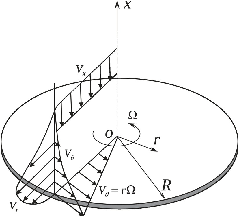
Figure 4.1 Free disk pumping.
Schlichting (1979) presents von Karman momentum integral boundary layer solutions for both laminar and turbulent boundary layers in a free rotating disk. Here we present the key results only from the turbulent boundary solutions. For the one-seventh power law profile in the boundary layer, assuming turbulent boundary layer right from r = 0r=0, the fee disk pumping mass flow rate is given by
 (4.1)
(4.1)which may be alternatively written as
 (4.2)
(4.2)where Re = ρR2Ω/μRe=ρR2Ω/μ is the disk rotational Reynolds number based on the disk radius RR. Although a free rotating disk is not found in a gas turbine design, Equations 4.1 or 4.2 estimates the upper limit for the disk pumping flow. Note that, for a laminar boundary layer, the disk pumping flow rate varies as r2r2, see for example Schlichting (1979). Because the disk area also varies as r2r2, the axial velocity of entrainment remains uniform over the disk. For the turbulent boundary layer, however, the disk pumping flow rate according to Equation 4.2 varies as r2.6r2.6, as a result, the axial velocity of the entrained flow increases with radius for an incompressible flow.
Another design parameter of interest is the torque produced by the tangential wall shear stress distribution on the rotor disk. This torque for one side of the disk wetted by the fluid is given by
 (4.3)
(4.3)which from the solution, expressed in terms of the moment coefficient, yields
 (4.4)
(4.4)Because the disk is rotating with angular velocity ΩΩ, the total disk torque computed from Equation 4.3 will impart windage equal to ΓΩΓΩ to the boundary layer flow (pumping flow).
4.1.2 Disk Pumping Beneath a Forced Vortex
Figure 4.2a shows the boundary layer flows on a rotating disk when the fluid outside the boundary layer itself rotates as a forced vortex at a fraction of the disk angular velocity. The ratio of fluid core angular velocity and the disk angular velocity is represented by the swirl factor SfSf. At Sf = 0Sf=0, the flow field of Figure 4.2a reverts to that of the free rotating disk shown in Figure 4.1 and yields the maximum pumping flow rate in the boundary layer. When Sf = 1Sf=1, the fluid gets into solid-body rotation with the disk with no pumping flow.

Figure 4.2 (a) Disk pumping beneath a forced vortex and (b) fraction of free disk pumping mass flow rate versus swirl factor.
Newman (1983) extends the momentum integral method of von Karman, presented in Schlichting (1979) for a free rotating disk, to cases for which the outer flow is rotating at a constant angular velocity. Boundary layers for both radial and tangential velocities are assumed turbulent right from r = 0r=0. From the solution results presented by Newman (1983), we obtain the following formula to compute disk pumping mass flow rate for the one-seventh power law velocity profile assumed in the boundary layer:
 (4.5)
(4.5)where ζζ, given by Equation 4.6, is the fraction of the free disk pumping mass flow rate computed by Equation 4.1.
As shown in Figure 4.2b, ζζ depends strongly on the swirl factor SfSf, yielding the maximum value of the disk pumping mass flow rate for Sf = 0Sf=0 and no pumping for Sf = 1Sf=1. Equation 4.5 is a useful design equation to estimate pumping flow rate on a rotor surface between two radii.
4.1.3 Rotor Disk in an Enclosed Cavity
Figure 4.3 shows a disk rotating in a stationary housing with zero inflow and outflow. As a result of no-slip boundary conditions, the fluid assumes local velocity of the rotor and stator in contact. The rotor disk acts like a bladeless compressor or a pump (incompressible flow) and pumps the fluid radially outward. Because the disk pumping flow increases radially outward, it is continuously being fed (axial flow from the stator boundary layer to the rotor boundary layer) from the radially inward flow along the stator. The presence of the stationary shroud makes the stator torque somewhat higher than the rotor torque. As a result, the fluid core is expected to rotate at less than half of the disk angular velocity (Sf < 0.5Sf<0.5). As the gap between the stator and the rotor decreases, the fluid core will tend to rotate at Sf = 0.5Sf=0.5. The radial static pressure gradient in the enclosure will be established corresponding to the forced vortex with Sf = 0.5Sf=0.5.

Figure 4.3 Rotor disk in an enclosed cavity.
Although the torque on the stator surface does not do any work, there is continuous work transfer into the fluid from the rotor disk. As a result, the fluid temperature within a perfectly insulated enclosure will rise continuously.
4.2 Cavity
The rotor-rotor and rotor-stator cavities are the most dominant and ubiquitous features of internal flow systems of gas turbines. Assuming a turbulent cooling and sealing flow in these systems, the interplay of flow behavior on a rotor surface, a stator surface, and the mass flow rate associated with radially outward or inward flow is responsible for a variety of flow features found in theses cavities. A good understanding of these flow features is the key to their one-dimensional modeling for the flow network simulation of these internal flow systems.
A rotor surface tends to pump the flow radially outward and acts like a bladeless compressor if the adjacent fluid core rotates at a fraction of the disk angular velocity and like a bladeless turbine if the fluid core co-rotates faster than the disk. In the first case, the energy transfer occurs from the rotor disk to the fluid and in the second case from the fluid to the disk. On the disk itself, tangential velocity varies linearly with radius. Stator torque acts to reduce the angular momentum of the flow regardless of the flow direction and rotation. The stator does not partake directly in the energy transfer to or from the fluid. For a small flow influenced by rotor and stator torques, the core behaves like a forced vortex rotating at a fraction (around 0.5) of the rotor disk angular velocity. For a large flow, which is not influenced by rotor and stator torques, the flow behaves more like a free vortex, keeping a nearly constant angular momentum. In this case, the angular velocity of a radially outward flow decreases downstream and for a radially inward flow increases in the flow direction, at times exceeding the rotor angular velocity.
In general, a fluid flow seeks the path of least resistance. In a rotating flow, the difference between the angular velocity of the flow and that of the wetted wall determine the torque. If the wall rotates faster than the fluid, it will increase the flow angular momentum. If the wall angular velocity is less than that of the fluid, the torque produced will decrease the flow angular momentum. Accordingly, the stator torque always reduces the angular momentum of the adjacent fluid flow.
4.2.1 Rotor-Stator Cavity with Radial Outflow
Figure 4.4 shows a rotor-stator cavity with a superimposed radial outflow. For a small outflow rate, shown in Figure 4.4a, the flow streamlines, fully meeting the demand of the induced pumping flow, are along the rotor surface. At a radius where the disk pumping flow rate exceeds the superimposed flow rate, the fluid is entrained from the radially inward flow induced on the stator surface to make up for the difference, as shown in the figure. For a large superimposed radially outflow, exceeding the disk pumping flow, no radially inward flow on the stator surface occurs, as shown in Figure 4.4b.

Figure 4.4 Schematic of a rotor-stator cavity with superimposed radial outflow: (a) small outflow rate and (b) large outflow rate.
4.2.2 Rotor-Stator Cavity with Radial Inflow
Figure 4.5 shows a rotor-stator cavity with a superimposed radial inflow. For a small inflow rate with Sf < 0.5Sf<0.5, shown in Figure 4.5a, the flow enters the cavity along the stator surface. Some of this flow is peeled off by the rotor to satisfy its pumping flow requirement, featuring a flow reversal over a part of the cavity near the rotor surface. At a lower radius, the flow starts swirling faster like a free vortex and preferably migrates to descend down the rotor surface so as to minimize the overall wall shear force opposing it. This part of the rotor disk, where the fluid is flowing radially inward, acts like a bladeless turbine.

Figure 4.5 Schematic of a rotor-stator cavity with superimposed radial inflow: (a) small inflow rate and (b) large inflow rate.
In case of a large radial inflow, shown in Figure 4.5b, the flow behaves more like a free vortex and preferentially flows down the rotor surface so as to minimize the overall shear force. The entire rotor disk in this case behaves like a bladeless radial turbine with work transfer from fluid to the rotor.
4.2.3 Rotating Cavity with Radial Outflow
Figure 4.6 shows the complex shear flow streamlines of a radial outflow in the cavity between two rotating disks. The axial flow entering the cavity through the upstream disk undergoes a sudden geometric expansion. The growth of the outer shear layer of the annular jet occurs through entrainment of the pressure-gradient-driven backflow from the downstream stagnation region. This creates the primary recirculation region shown in the figure. The size and strength of this recirculation region are found to depend mainly on the flow rate and rotational speed as discussed in Sultanian and Nealy (1987). The entering axial flow turns 90 degrees over the concave corner and flows radially outward, aided in part by frictional pumping over the downstream disk induced by its rotation. A part of the flow (almost half in this case!) turns back toward the upstream disk and moves radially outward as a result of similar pumping action over that disk.

Figure 4.6 Schematic of a rotating cavity with superimposed radial outflow.
4.2.4 Rotating Cavity with Radial Inflow
In the rotating cavity shown in Figure 4.7, we have a radial inflow. Like the case of radial outflow, the rotating cavity features essentially four regions. Both the source region at the inlet and sink region at the outlet are complex shear flows. The core in the mid-section of the cavity features nearly zero axial and radial velocities, and it is bounded by Ekman boundary layers on both disks. These boundary layers are essentially nonentraining. In essence, the flow entering the rotating cavity splits almost in half and flows down radially on each disk with no intermediate entrainment. Because we normally associate disk pumping with a radially outward flow in the disk boundary layer, the flow features shown in Figure 4.7 may appear somewhat counterintuitive to some.

Figure 4.7 Schematic of a rotating cavity with superimposed radial inflow.
4.3 Windage and Swirl Modeling in a General Cavity
A major task in the design of gas turbines is to compute windage and swirl distributions throughout the path of an internal flow system. These distributions are needed to determine the thermal boundary conditions for structural heat transfer analysis and for establishing static pressure distributions for axial load calculations. Figure 4.8 shows the schematic of a general gas turbine cavity and its key features. This cavity includes multiple axisymmetric surfaces, which may be rotating, co-rotating, counter-rotating, or stationary. Each disk surface may comprise of radial, conical, and horizontal surfaces; for example, shown for surface 2 in the figure, and may feature three-dimensional protrusions, called bolts, which tend to destroy the overall symmetry of the cavity about the axis of rotation. Additionally, the cavity may have multiple inflows and outflows with different swirl, pressure, and temperature conditions.

Figure 4.8 Schematic of a general gas turbine cavity and its key features.
Because the flow field in the general cavity shown in Figure 4.8 is highly complex and three dimensional, a 3-D CFD appears to be the only viable analytical method for its analysis and predictions. Such an analysis may not, however, support the shrinking design cycle time and realizing a robust design requiring multiple runs to account of statistical variations in boundary conditions. In the following sections, we present a 1-D flow modeling methodology based on the large control volume analysis for a general gas turbine cavity encountered in design. Because the methodology uses some of the published correlations to compute torque of stator and rotor surfaces, it behooves the readers (designers) to modify them in their design applications based on their design validation studies.
Daily and Nece (1960) studied, both experimentally and theoretically, the fundamental fluid mechanics associated with the rotation of a smooth plane disk enclosed within a right-cylindrical chamber, as shown in Figure 4.9. In this investigation, the torque data were obtained over a range of disk Reynolds numbers from Re = 103Re=103 to Re = 107Re=107 for axial clearance to disk radius ratios from G = 0.0127G=0.0127 to G = 0.217G=0.217 for a constant small radial tip clearance; the velocity and pressure data were obtained for both laminar and turbulent flows. The tangential and radial velocity profiles are schematically shown in Figure 4.9a for the case of merged boundary layers and in Figure 4.9b for the case of separate boundary layers.

Figure 4.9 Rotor disk in an enclosed cavity: (a) merged boundary layers (Regimes I and III) and (b) separate boundary layers (Regimes II and IV).
The study of Daily and Nece (1960) identifies the existence of the following four basic flow regimes, which are delineated in Figure 4.10 for various combinations of ReRe and GG. The rotor disk moment coefficient in each regime is summarized as follows:
Regime I: Laminar flow with merged boundary layers (small clearance)

Regime II: Laminar flow with separate boundary layers (large clearance)

Regime III: Turbulent flow with merged boundary layers (small clearance)

Regime IV: Turbulent flow with separate boundary layers (large clearance)


Figure 4.10 Delineation of four flow regimes in the flow of a disk rotating in an enclosed cavity (Daily and Nece, 1960).
Regime IV is generally considered relevant for gas turbine design applications. For our 1-D modeling of a general cavity, we make use of the rotor and stator moment coefficients proposed by Haaser, Jack, and McGreehan (1988) and extend them for partial disks, which may be co-rotating and counter-rotating with arbitrary angular velocities.
Based on the actual gas turbine test experience and the experimental data of Daily and Nece (1960); Haaser, Jack, and McGreehan (1988) proposed the empirical correlation for the shear coefficient on one side of the rotor disk as
and that on one side of the stator disk as
where the full disk Reynolds number (Re=ρΩRo2/μ ) has been modified to
 (4.13)
in order to use the correlations for a partial disk (Ri>0Ri>0). Note that Equations 4.11 and 4.12 have been deduced from the following moment coefficient correlations assumed for the full disk by assuming a uniform radial distribution of the tangential shear stress. Under this assumption, the shear coefficient and moment coefficient are related as follows:
 (4.14)
Using Equation 4.14, we obtain the moment coefficient equation from Equation 4.11 for the partial rotor disk as
 (4.15)
for the full rotor disk as
for the partial stator disk as
 (4.17)
and for the full stator disk as
Equations 4.15 and 4.16 for the rotor disk or Equations 4.17 and 4.18 for the stator disk of outer radius RoRo yield the following relation for the ratio of the torque for a partial disk with Ri>0Ri>0 to that for a full disk with Ri = 0Ri=0:
 (4.19)
The plot of Equation 4.19 in Figure 4.11 shows that for Ri/Ro ≤ 0.5Ri/Ro≤0.5, the equation yields Γpartial>ΓfullΓpartial>Γfull, which is physically unacceptable. To mitigate this problem, we make the assumption that, instead of a constant tangential shear stress over the disk, as assumed in Haaser, Jack, and McGreehan (1988), the local shear coefficient of the tangential shear stress is constant, giving
 (4.20)
Figure 4.11 Variation of disk torque ratio (Γpartial/ΓfullΓpartial/Γfull) with radius ratio (Ri/RoRi/Ro).
Thus, from Equations 4.16 and 4.20, we obtain for the rotor disk
 (4.21)
Similarly, from Equations 4.18 and 4.20, we obtain for the stator disk
 (4.22)
Based on Equations 4.21 and 4.22, we obtain for rotor and stator disks the following relation
 (4.23)
which is plotted in Figure 4.11. The figure shows that the anomaly associated with Equation 4.19 is absent from Equation 4.23.
In using Equations 4.21 and 4.22 for calculating local tangential shear stress on the rotor surface and stator surface, respectively, one is expected to use the dynamic pressure 0.5ρΩ2r20.5ρΩ2r2. For a general 1-D modeling of cavities, it is more appropriate to use the fluid tangential velocity relative to the surface to compute the dynamic pressure, which for the rotor becomes 0.5ρ(1 − Sf)2Ω2r20.5ρ1−Sf2Ω2r2 and for the stator 0.5ρSf2Ω2r2 . Accordingly, Equations 4.21 and 4.22 are recast as follows:
where Re=ρRo2Ω/μ .
.
Let us now consider the 1-D steady adiabatic flow modeling in a simple rotor-stator cavity shown in Figure 4.12a. With ṁin=ṁout=ṁ , the steady continuity equation in the cavity is satisfied. Because the flow is assumed adiabatic, the change in fluid total temperature occurs entirely as a result of work transfer from the rotor. The stator torque participates in the torque-angular momentum balance only but not directly in the energy transfer with the fluid. To capture accurate variations of flow properties in the cavity, we divide it into a number of control volumes. For the control volume k whose inlet surface is designated by j and the outlet surface by j+1, we write the following angular momentum equation:
 (4.26)
Figure 4.12 Cavity with throughflow: (a) rotor-stator cavity, (b) cavity of co-rotating disks, and (c) cavity of counter-rotating disks.
Assuming a forced vortex core with swirl factor SfkSfk such that Sfj + 1 = SfkSfj+1=Sfk and substituting

and

in Equation 4.26, we obtain
 (4.27)
which is a transcendental equation in the unknown SfkSfk.
Note that in the marching solution from the cavity inlet to outlet we have Sfj = Sfk − 1Sfj=Sfk−1, which is obtained from the solution for the upstream control volume. One can use the regula falsi method, presented, for example, in Carnahan, Luther, and Wilkes (1969), as a robust and fast iterative solution technique for obtaining SfkSfk from Equation 4.27; see also Appendix D.
Knowing SfkSfk in the control volume, the static pressure change from inlet to outlet can be obtained using the radial equilibrium equation
 (4.28)
Using an average value of density ρ¯=0.5ρj+ρj+1 for the control value, Equation 4.28 can be integrated to yield

Thus, the change in fluid total temperature as a result of windage in the control value can be obtained using the equation

In the foregoing derivations, we have tacitly assumed that Sf < 1Sf<1 in which case the work transfer occurs from the rotor disk to the fluid. For Sf>1Sf>1, however, the fluid does work on the rotor. In the following section, we will account for this possibility in the modeling of a general cavity with arbitrary inflow conditions.
Figures 4.12b and 4.12c depict a cavity with two rotor disks, which are either co-rotating or counter-rotating. If we set Ωref = 0Ωref=0, these cavities revert to that of Figure 4.12a. Considering the rotor with the highest angular velocity as the reference rotor in a multirotor cavity and using its angular velocity (ΩrefΩref) to normalize other rotor and fluid angular velocity, we can easily extend Equation 4.24 to express the local shear coefficient for any rotor in the cavity as
where


Note that the local dynamic pressure to be used in conjunction with Equation 4.29 equals 0.5ρβ−Sf2Ωref2r2 . Further note that Equation 4.29 is applicable to all rotors in the cavity, including the reference rotor with β = 1β=1.
For the stator surface, we re-write Equation 4.25 as
4.3.1 Arbitrary Cavity Surface Orientation: Conical and Cylindrical Surfaces
A cavity may have a rotor or stator disk comprising conical and cylindrical surfaces. For the conical part of a rotor disk we use the shear stress coefficient correlation given by Equation 4.29, and if the conical surface is a part of a stator disk, we use Equation 4.30 to compute its local shear coefficient. For the conical surface segment of the rotor disk, shown in Figure 4.13a, we express its torque as
 (4.31)
where


Figure 4.13 (a) Disk with a conical surface and (b) disk with a cylindrical surface.
For the corresponding conical surface segment of a stator disk, we express its torque as
 (4.32)
where

For the cylindrical rotor surface segment shown in Figure 4.13b, we adopt the shear stress coefficient correlation proposed by Haaser, Jack, and McGreehan (1988), extended for a rotor in addition to the primary rotor
where

Using Equation 4.33, the torque of the cylindrical surface segment of the rotor can be obtained as follows:
 (4.34)
For the corresponding cylindrical surface segment of a stator disk, we extend Equation 4.12 for the shear coefficient to the generalized form
which yields the corresponding torque as
 (4.36)
4.3.2 Bolts on Stator and Rotor Surfaces
Bolts are three-dimensional protrusions on rotor and stator surfaces. They significantly influence both the windage generation and swirl distribution in the cavity. The bolt-to-bolt spacing has a profound effect of its drag force. As the one bolt falls in wake of its upstream bolt, relative to the tangential flow velocity, its drag contribution decreases. Figure 4.14a shows bolts on a disk with small bolt-to-bolt interference, while the increased number of bolts shown in Figure 4.14b result in higher bolt-to-bolt interference.

Figure 4.14 (a) Disk with bolts with small interference and (b) disk with bolts with large interference.
Following the approach of Haaser, Jack, and McGreehan (1988), the torque as a result of bolts in an axisymmetric cavity is computed as follows:
Bolts on rotor surface:
 (4.37)
Bolts on stator surface:
 (4.38)
where
Nb≡Nb≡ Number of bolts
h ≡ Bolt height from the disk surface
b ≡ Bolt width along the radial direction
CDb≡CDb≡ Baseline drag coefficient of each bolt (≈ 0.6)
Rb≡Rb≡ Bolts pitch circle radius
Ib≡Ib≡ Bolts interference factor (a function of s/ds/d, see Figure 4.14a)
Based on the empirical data presented in Hoerner (1965), the following approximate correlations are obtained to compute IbIb as a function of s/ds/d:
For 1≤sd<2
 (4.39)
For 2≤sd<7
 (4.40)
These correlations yield Ib = 0.25Ib=0.25 for s/d = 1s/d=1 and Ib = 1.0Ib=1.0 for s/d>6s/d>6.
4.4 Compressor Rotor Cavity
Axial compressors of gas turbines for aircraft propulsion and power generation feature multiple stages to achieve high compression ratio (20–40) needed in today’s high-performance engines. Compressed air temperatures in aft stages of the compressor tend to be very high. As a result of increasing air density along the compressor flow path, its annulus area also decreases with smaller vanes and blades. The thermal growth of compressor rotor disks relative to their outer casing play an important role in determining the blade-tip clearances, which impact compressor aerodynamic performance. During transients of engine acceleration and deceleration, rim-to-bore temperature gradients in each disk determine its low cycle fatigue (LCF) life. This calls for a transient conduction heat transfer analysis of each rotor disk with convection boundary conditions from the air in the cavity (called rotor cavity) formed with the adjacent disk. These rotor cavities are found in all shapes and sizes, some of them are completely closed, while others are cooled with an axial throughflow, called bore flow. Completely closed compressor rotor cavities are generally found in industrial gas turbines. In aircraft engines, except for initial stages of a high-pressure compressor (HPC), the rotor cavities feature a bore flow, which is designed to influence the rotor-tip clearances for better compressor aerodynamic performance and higher LCF life of each rotor disk.
Figure 4.15 schematically shows a compressor rotor cavity with bore flow. Without the bore flow, the rotor cavity may be considered a closed cavity. Because the static pressure at the vane exit is higher than that at its inlet, a reverse flow through each inter-stage seal in the main flow path occurs. Note that the windage generated in these inter-stage seals of an axial-flow compressor significantly change the thermal boundary conditions on rotor surfaces exposed to the main flow path.

Figure 4.15 Schematic of an axial compressor rotor cavity.
4.4.1 Flow and Heat Transfer Physics
In order to better understand the unsteady and three-dimensional nature of the centrifugally-driven buoyant convection (CDBC) in a typical compressor rotor cavity, schematically shown in Figure 4.15, let us first look at the spin-up and spin-down flow behavior in a closed adiabatic rotor cavity shown in Figure 4.16. When we impulsively rotate a closed cavity to the steady angular velocity ΩΩ, shown in Figure 4.16a, the fluid initially at rest inside the cavity eventually reaches a solid-body rotation with the cavity walls. During the transient, the angular momentum from the walls is transferred to the fluid through the action of viscosity and no-slip boundary condition at the walls. On the cylindrical surface parallel to the axis of rotation, we have negligible axial pressure gradients and the viscous boundary layer (called Stewartson boundary layer) grows radially inward. Each disk surface, which is normal to the axis of rotation, behaves like a free disk rotating adjacent to a nonrotating fluid, discussed earlier in this chapter, and results in the radially-outward pumping secondary flow in the Ekman boundary layer, continuously entraining fluid from the core.

Figure 4.16 (a) Fluid spin-up from rest in a rotating closed cavity and (b) spin-down of fluid under solid-body rotation to rest in a nonrotating closed cavity.
Let us try to physically understand how the radially-outward secondary flow is initiated during spin-up. Being stationary, the core features uniform zero pressure gradient, which is also imposed on the boundary layers on the cavity surfaces. Within the disk boundary layer, the fluid attains angular momentum and causes centrifugal body force, which is balanced by an adverse radial pressure gradient (dPs/dr=ρrΩf2 ). To ensure zero net pressure gradient within the boundary layer, as imposed from the core fluid, a favorable radial pressure gradient is created, which causes increase in radial momentum flow while also overcoming the opposing viscous force from the radial wall shear stresses. This radial disk pumping flow grows by entraining fluid from the core. Thus, to satisfy continuity, circulating flows develop in the meridional plane, as shown in Figure 4.16a.These circulating flows speed up the transient process and the whole system reaches the state of solid-body rotation by an order of magnitude faster than through viscous diffusion alone. If the disks were frictionless, the secondary flow would seize to exist, and the steady state would take place through the growth of the Stewartson boundary layer alone.
During spin-down from solid-body rotation, when the rotor cavity walls are suddenly stopped, as shown in Figure 4.16b, secondary flows in each meridional plane within the Ekman and Stewartson boundary layers circulate in the directions opposite to those in the spin-up process. The occurrence of a radially inward flow in the Ekman boundary layer on each disk can be physically explained as follows. The fluid core initially in solid-body rotation has a radial pressure gradient (dPs/dr = ρrΩ2dPs/dr=ρrΩ2), which is imposed on each disk boundary layer. Because the fluid in the boundary layer has lower angular velocity than that in the core at the same radius, it experiences a net radially-inward pressure force causing it to flow toward the axis of rotation. Thus, circulating secondary flows develop in the cavity to satisfy continuity.
The spin-down process with its interesting feature of radially-inward flow in the Ekman boundary layer can be easily demonstrated in a simple home experiment. Let us take a cup of water and drop in it a few mustard seeds. With a straw, let us now vigorously stir the water and bring it to a state of solid-body rotation. When we stop stirring and pull the straw out, the water spins down to rest within a minute or so. During the spin-down process, we notice that the mustard seeds, which were mostly rotating away from the axis of rotation, collect at the bottom of the cup, not at the periphery but near the center (around the axis of rotation). The mustard seeds are carried there by the radially-inward flow at the bottom surface.
It may be noted here that, during the spin-up process, the work transfer (windage) from the adiabatic cavity walls will somewhat raise the total temperature of the cavity fluid. In the steady state of solid-body rotation, the fluid features a radial pressure gradient and becomes isothermal. This is true even for a compressible fluid like air. For an adiabatic spin-down, no work transfer occurs, and the fluid total temperature remains constant.
When the annular bore flow passes over the open compressor rotor cavity, shown in Figure 4.15, it undergoes a sudden geometric expansion and may impinge on the web region of the downstream disk. The jet expansion over the cavity results in a toroidal vortex, which recirculates in the axial direction and moves in solid-body rotation with the outer core flow in the cavity under adiabatic conditions. Unlike a driven cavity flow, the radial extent of the toroidal vortex is confined to the web region. For the case of disks temperature being different from that of the bore cooling air flow, CDBC drives a very complex flow structure in the rotor cavity. In their comprehensive review of buoyancy-induced flow in rotor cavities, Owen and Long (2015) note that, for the situation when the temperature of the disks and shroud is higher than that of the air in the cavity, the unstable and unsteady three-dimensional cavity flow features sources (high-pressure regions) and sinks (low-pressure regions), which in the rotating coordinate system (disks rotating counterclockwise, aft looking forward) appear as anti-cyclonic (rotating clockwise) and cyclonic (rotating counterclockwise) flows, respectively. In addition, a part of the axial bore flow enters the cavity through radial arms and return via Ekman layers on the disks. There is little hope of micro-modeling this cavity flow as a means to perform heat transfer calculations for design applications. In the next section, we present a practical approach to 1-D heat transfer modeling of compressor rotor cavities under CDBC.
4.4.2 Heat Transfer Modeling with Bore Flow
In free convection, both the flow and heat transfer are intricately coupled, that is, one depends on the other. Our daily experience involves free convection largely driven by the gravitational force field with a nearly constant acceleration (g = 9.81 m/s2g=9.81m/s2). In the chimney attached to the fireplace in our homes, we know that the hot air rises and the cold air sinks to satisfy continuity, generating a free convection flow, which we call gravitationally-driven buoyant convection (GDBC). As we know, water has its maximum density at 4oC4oC. In winter, when a lake starts to freeze, GDBC plays the role in ensuring that the water stays in the liquid phase to save marine life below the frozen top layer, which also acts as a good thermal insulator. When we have cold air next to a hot vertical wall, the free convection flow goes upward in the wall boundary layer. When the vertical wall is colder than the adjacent air, the free-convection flow comes downward in the wall boundary layer. For a downward facing horizontal wall, however, GDBC happens only when the wall is colder than the air; when this wall is hotter than the air, the flow is stably stratified with no GDBC.
The acceleration associated with the centrifugal force in a rotating system is given by gc = rΩ2gc=rΩ2, which varies directly as the radius of rotation and as the square of the angular velocity. At r = 0.5 mr=0.5m, for a cavity rotating at 3000 rpm, we have gc/g≈5000gc/g≈5000, which clearly shows the strength of CDBC in a compressor rotor activity vis-à-vis GDBC for similar temperature differences between cavity surface and the surrounding air. In the case of CDBC, cold fluid moves radially outward and warm fluid moves radially inward. Thus, when the wall is hotter than the fluid, the fluid flows radially inward in the disk boundary layer, and, when the wall is colder than the fluid, it flows radially outward in the boundary layer.
For 1-D heat transfer modeling of a compressor rotor cavity with a bore flow, shown in Figure 4.17, we divide the cavity in multiple control volumes, compute the convective heat transfer in each control volume and find the total convective heat transfer rate (Q̇c ), which becomes the boundary condition for the steady-flow energy equation over the bore CV to determine the air total temperature change from inlet to outlet. Accordingly, we can write
 (4.41)
Figure 4.17 1-D Heat transfer modeling of compressor rotor cavity with bore flow.
For calculating the convective heat flux q̇c=hTw−Taw from each wall of the cavity CV, we need three quantities: wall temperature (TwTw); adiabatic wall temperature (TawTaw), which acts as the fluid reference temperature; and heat transfer coefficient (hh), which is obtained from a specified empirical correlation. In this multitemperature problem, it is not obvious which temperature we should use as the appropriate adiabatic wall temperature. In the present approach, we make use of the fact that, under adiabatic conditions, the rothalpy will remain constant for any excursion of the fluid in solid-body rotation within the rotor cavity. Thus, we can write
 (4.42)
where rr is the central radius of a cavity control volume and rborerbore corresponds to the mean radius of the bore flow. Owen and Tang (2015) also suggest the use of Equation 4.42 for the fluid reference temperature to compute the convective heat transfer between the cavity wall and air in CDBC. They have, however, arrived at this equation using the compressibility effects and invoking the isentropic relationship between the pressure ratio and temperature ratio at two points.
As to the empirical heat transfer correlations for CDBC on the disk and cylindrical rim surfaces, we present here a set of standard correlations for GDBC from McAdams (1954). These correlations conform to the common equation form
The coefficient C and the exponent m for the Rayleigh number RaRa used in Equation 4.43 for various situations are tabulated in Table 4.1. In view of the geometric complexity of a compressor rotor cavity with arbitrary temperature distribution on its bounding surfaces, the empirical correlations suggested by Equation 4.43 are to be treated as nominal correlations for initial modeling purposes only. Such correlations must be later refined and established for a consistent design practice from extensive thermal surveys for various designs. These empirical correlations then become proprietary to the original equipment manufacturer and do not belong to a textbook.
Table 4.1 Constants C and m used in Equation 4.43
| Physical situation | Ra range | C | m |
|---|---|---|---|
| Vertical surface | 104 − 109104−109 | 0.59 | 14 |
| Vertical surface | 109 − 1012109−1012 | 0.13 | 13 |
| Horizontal surface (Tw>TawTw>Taw, CDBC) | 105 − 2 × 107105−2×10⁷ | 0.54 | 14 |
| Horizontal surface (Tw>TawTw>Taw, CDBC) | 2 × 10⁷ − 3 × 10102×107−3×10¹⁰ | 0.14 | 13 |
| Horizontal surface (Tw < TawTw<Taw, CDBC) | 3 × 10⁵ − 3 × 10103×105−3×10¹⁰ | 0.27 | 14 |
Note that for the correlations in Table 4.1 with m = 1/3m=1/3, which are to be used for a turbulent boundary layer, the resulting heat transfer coefficients become independent of the characteristic length.
4.4.3 Heat Transfer Modeling of Closed Cavity
The foregoing heat transfer modeling of a compressor rotor cavity with the bore flow can be easily extended for the situation of a closed cavity with no bore flow. When the cavity is closed, it essentially operates under unsteady heat transfer. The mass m˜c of air in the cavity remains constant. For each time step ΔtΔt we make a quasi-steady-state assumption and use a fictitious bore flow m˜̇bore=m˜/Δt
 . If TtR(t)TtRt is the air total temperature in the rotor reference frame at the beginning of the time step, then the corresponding air temperature at the end of the time step can be computed as
 (4.44)
where the total convective heat transfer Q̇c for the closed cavity is to be computed just as we did for the cavity with bore flow in the previous section, assuming TtRin = TtR(t)TtRin=TtRt.
4.5 Preswirl System
For internal cooling of turbine blades subjected to high temperatures in the main flow path, the design intent is always to keep the extracted compressor air (used as coolant) as cool as possible at the specified total pressure at the blade root. In its journey from the compressor bleed point to turbine blade inlet, the cooling air will be heated by heat transfer from the stator and rotor surfaces and work transfer from rotor surfaces. Under adiabatic conditions, the cooling air total temperature remains constant over the static structure. When we bring this air onboard the turbine rotor for blade cooling, its total temperature relative to the rotor increases as a result of work transfer from the rotor. This is an undesirable effect on the blade cooling air temperature. A simple technique to avoid this temperature increase is to preswirl the air in the static structure using a number of nozzles, as shown in Figure 4.18. When the coolant air is preswirled to the rotor angular velocity, it enters the holes in the cover plate with no change in its absolute total temperature, as a result, there is no loss in turbine power with simultaneous reduction in the coolant air total temperature relative to the rotor at the same radius.

Figure 4.18 Schematic of a preswirl system for turbine blade cooling air.
4.5.1 Flow and Heat Transfer Modeling
As shown in Figure 4.18, the blade cooling air flow from the preswirl nozzles interacts with a complex flow region in the stator-rotor cavity before it enters the rotor cavity between the cover plate and the rotor disk at point 2. At this point, the flow is brought onboard the rotor with solid-body rotation. From point 2 to point 3 in the rotor cavity, the core flow behaves likes a generalized vortex within a complex shear flow. The flow eventually reaches the blade root at point 4 at the design-specified conditions of relative total pressure and temperature for blade internal cooling with the adequate backflow margin so as to prevent any ingestion of hot gases through the blade film cooling holes.
Let us now turn our attention to how the coolant air total temperature changes in a preswirl system from nozzle exit (point 1) to blade inlet (point 4), the first being in the stator reference frame (SRF) and the second in the rotor reference frame (RRF). Under adiabatic conditions with constant cpcp for the coolant air, we can invoke the concept of rothalpy to relate total temperatures in SRF and RRF at any point as
 (4.45)
where the swirl factor Sf = Vθ/(rpΩ)Sf=Vθ/(rpΩ). Equation 4.45 shows that for Sf1 = 0.5Sf1=0.5; that is, the air is rotating at half the rotor speed, we obtain TtR = TtSTtR=TtS. For Sf = 0Sf=0, TtRTtR is higher than TtSTtS by the dynamic temperature corresponding the solid-body rotation (r2Ω2/2cpr2Ω2/2cp), and, for Sf = 1Sf=1, it is lower than TtSTtS by the same amount and equals the static temperature.
With reference to Figure 4.18, let us now evaluate the reduction in the coolant air total temperature from point 1 to point 4 under no heat transfer. At point 1, Equation 4.45 yields
 (4.46)
Because the rothalpy remains constant in RRF for an adiabatic flow, we obtain
 (4.47)
Combining Equations 4.46 and 4.47 yields
 (4.48)
where θ may be interpreted as the blade cooling air temperature reduction coefficient as a result of preswirl nozzles. When we multiply the dynamic temperature of solid-body rotation, rb2Ω2/(2cp) , at point 4 by θ, we obtain (TtS1 − TtR4)(TtS1−TtR4).
Equation 4.48 and its plot in Figure 4.19 show that θ varies linearly with the swirl factor Sf1Sf1 at the preswirl nozzle exit and as the square of the radius ratio rb/rprb/rp. Negative values of θ imply that TtR4>TtS1TtR4>TtS1. For Sf1 = 1Sf1=1, positive values of θ occur only for rb/rp>0.707rb/rp>0.707. At first, it appears from Figure 4.19 that over-spinning the blade cooling air flow to Sf1>1Sf1>1 in the preswirl nozzles will have added beneficial effect of reducing its relative total temperature at the blade inlet. But the gas turbine designer must balance this against the additional reduction in static pressure, which may not be recovered downstream, in order to generate higher dynamic pressure associated with the higher swirl factor at the nozzle exit.

Figure 4.19 Variation of θ with preswirl-to-blade inlet radius ratio rb/rprb/rp for various exit swirl factor Sf1Sf1.
Let us now evaluate the loss in turbine work in the transfer process from preswirl nozzles exit to blade inlet. Because the cooling air attains the solid-body rotation at point 4, we can equate the rothalpy expressed in SRF at point 1 to that at point 4, giving
 (4.49)
where θ˜ may be interpreted as the turbine work loss coefficient. Combining this equation with Equations 4.48 yields
 (4.50)
It is interesting to note from Equation 4.50 that the design goal of higher value of θ and lower value of θ˜ is achieved simultaneously. For θ˜>1 , which implies θ < 1θ<1, the transfer system exhibits a compressor-like behavior, while for θ˜<1
 , which implies θ>1θ>1, the system behaves like a turbine. In the design of a blade cooling system, it is important to ensure that the required supply pressure at the blade inlet is met even with a slight increase in θ˜, using the turbine rotor to provide the needed pumping power.
The radial location of preswirl nozzles is an important design consideration. For the same value of Sf1Sf1, Vθ1Vθ1 will higher, the higher the radius. This in turn will require higher extraction of dynamic pressure from the total pressure at the preswirl nozzles. Gas turbine designers also need to consider the impact of the preswirl radial location on rotor disk pressure distribution, which determines the axial rotor thrust.
For 1-D flow and heat transfer modeling of blade cooling air from point 1 to point 4, see Figure 4.19, we need to sequentially model the rotor-stator cavity between the inner and outer seals and the rotor cavity formed by the cover plate and the turbine disk up to point 3, using the methodology discussed in Section 4.3. Going from point 3 to point 4, we calculate the change in pressure and temperature using a forced vortex assumption of solid-body rotation of the turbine disk.
4.6 Hot Gas Ingestion: Ingress and Egress
Hot gas ingestion refers to ingress of hot gases from the main flowpath into the cavity, or wheel-space, formed between rotor and stator disks. This problem is most serious in the forward cavity of the first-stage turbine where hot gases exiting the vanes have the highest pressure and temperature. If the stator and rotor parts with no internal cooling, like disks, are exposed to hot gases by way of ingestion, their durability is considerably at risk. The design goal, over considerations of improved turbine efficiency and reduced specific fuel consumption, is always to eliminate or minimize the hot gas ingestion. It, therefore, behooves gas turbine designers to develop a good understanding of the primary factors and basic mechanism behind this phenomenon.
4.6.1 Physics of Hot Gas Ingestion
The phenomenon of hot gas ingestion is schematically shown in Figure 4.20. But for a small pressure loss in the combustor, the maximum total pressure at the trailing edge of the first stage vanes equals the compressor exit pressure. As a result of the dynamic pressure associated with the throughflow and tangential velocities needed for aerodynamic power extraction by the first stage blades, vane-to-vane static pressure distribution, which acts as the gas-path boundary condition for the cavity purge flow, is nonaxisymmetric and circumferentially periodic. As a result of this circumferentially asymmetric pressure distribution, characteristic of all gas turbines, the ingress of hot gases occurs wherever static pressure in the main flowpath is higher than that in the wheel-space. Egress into the main flow path occurs under a favorable pressure gradient over the regions where the gas path acts as the sink boundary condition for the purge air flow.

Figure 4.20 Schematic of hot gas ingestion in a gas turbine.
Unlike the compressor exit air going through the combustor and first stage vanes, where the total pressure decreases downstream, the purge air flow peeled off from the compressor exit loses its total pressure across multiple labyrinth seals but also gains it through work transfer from the rotor surfaces in contact. The cooling and sealing purge air flow typically maintains its swirl factor around 0.5 before reaching the rotor-stator cavity shown in Figure 4.20. The lower the purge air flow, the lower will be the loss in total pressure in the circuit from the compressor exit pressure and higher will be the favorable pressure gradient across the rim-seal opening. This, however, needs to be balanced against the excessive windage temperature rise in this internal flowpath.
If enough purge air flow is not feasible either as a result of source pressure constraint or to achieve the target cycle efficiency, the design intent shifts to restricting the hot gas ingestion to the outer parts of the stator and rotor structures; for example, the trench cavity and the buffer cavity shown in Figure 4.20. This is achieved through an innovative rim-seal design using a system of angel wings with adequate axial overlaps in conjunction with a trench cavity with appreciable radial overlap. For an improved conceptual design of these rim seals, it is important to understand how radial flows occur within boundary layers on the stator and rotor surfaces, separated by an inviscid vortex core.
Let us first consider the rotor boundary with an inviscid vortex core in the rotor-stator cavity shown in Figure 4.20. For the radially outward purge air flow in this cavity, the core is expected to rotate at around half the rotor speed (Sf≈0.5Sf≈0.5). The force of adverse pressure gradient in the core flow balances the centrifugal body force as a result of rotation (∂Ps/∂r=ρrSf2Ω2 ). At a radial location in the cavity, there is negligible pressure gradient in the axial direction, which is to say that the radial pressure gradient in the inviscid core flow is imposed on the rotor boundary layer. As a result of no-slip boundary condition, the fluid in contact with the rotor surface rotates in solid-body rotation. At the edge of the boundary layer, the fluid rotation equals that of the core flow. Accordingly, the average fluid tangential velocity is higher than that in the core, resulting in higher centrifugal body force and the consequent higher adverse radial pressure gradient in a small control volume encompassing the boundary layer. This difference in the radial pressure gradient in the boundary layer and in the core flow appears as a favorable radial pressure gradient in the rotor boundary layer, causing an increase in radial momentum flow, which is commonly known as disk pumping. Thus, the purge air flow in the rotor-stator cavity gets continuously entrained into disk pumping along the rotor. This pumping flow increases radially outward. If sufficient purge air flow is not available to satisfy the disk pumping flow, the flow will feed on itself through recirculation. From the flow physics behind disk pumping discussed here, it may be noted that, if the core flow rotates faster than the disk, it will induce a radially inward flow in the disk boundary layer, which may be counterintuitive based on our observational experience of free disk pumping.
For the boundary layer on the stator surface in the cavity with a rotating core flow, the radial pressure gradient argument presented in the foregoing will lead us to conclude a radially inward flow along the stator surface. Coming down radially, the flow in the stator boundary layer will continually detrain into the core flow. If we have a significant superimposed favorable pressure gradient in the core flow, we may prevent a radially inward flow in the stator boundary layer. Generally speaking, in the entire wheel space interfacing the main flowpath, the internal flow system of purge air flow features radially outward flows along all rotor surfaces and radially inward flows along all stator surfaces. Thus, the evidence of hot gas ingestion can be first observed on the stator surface in the rim seal area.
If the purge air flow rate equals the rotor disk pumping flow rate in the rotor-stator cavity, it will prevent hot gas ingestion into this cavity. Even with somewhat lower purge air flow, an angel wing on the rotor, see Figure 4.20, will act as an effective discourager and may prevent hot gases from entering the lower cavity. In the process of negotiating the turn around this angel wing, the radially outward boundary layer flow tends to create an aerodynamic stagnation point on the adjacent stator surface forcing the radially downward stator boundary layer flow to turn around rather than enter into the lower cavity. Note that if this angel wing were to be on the stator rather than on the rotor, it will be ineffective in protecting the rotor-stator cavity from the ingress of hot gases.
As shown in Figure 4.20, gas turbine designers use a rim seal system of rotor and stator angel wings with adequate radial and axial gaps and overlaps to restrict hot gas ingestion as close to the rim region as possible. In the rim seal design, the trench cavity with its significant radial overlap plays the key role in attenuating the asymmetry in pressure distribution in the main flowpath. Note that, going from vane exit to blade inlet over the wheel space, the flowpath pressure distribution also tends to become more axisymmetric.
From the foregoing discussion, we can glean the following primary factors that determine hot gas ingestion in a turbine stage:
Periodic vane/blade pressure field (nonaxisymmetric pressure distribution in the main flowpath of hot gases)
Disk pumping in the rotor-stator cavity
Rim seal geometry (radial and axial clearances and overlaps)
Purge sealing and cooling air flow rate
Some secondary factors, which also influence hot gas ingestion to some extent, include unsteadiness in 3-D flow field, and pressure fluctuations in the wheel space, and turbulent transport in the platform and outer cavity region.
For achieving higher engine performance, gas turbine designers may not have the luxury of minimum purge air flow rate needed to prevent hot gas ingestion by using a simple rim seal design. The competing effect of windage and hot gas ingestion must also be considered in design. When the purge flow is significantly reduced to achieve higher engine performance, the windage generated in the wheel space becomes critical to the creep life of many turbine components that support blades and vanes, which are necessarily protected using internal and film cooling, especially in the initial turbine stages. The design strategy to deal with the hot gas ingestion often follows the following sequence:
Establish the minimum cavity purge flow needed for acceptable windage temperature rise and heat transfer in the rotor-stator cavity.
Establish the gas path asymmetric pressure boundary conditions from an appropriate CFD solution.
Design a seal that will limit the ingress (hot gas ingestion) to trench (the first design target) and buffer cavities (the second design target if we can’t meet the first).
4.6.2 1-D Modeling
In view of the flow and heat transfer complexity associated with hot gas ingestion in gas turbines, one may be tempted to use 3-D CFD for its modeling and prediction. Except for providing improved understanding of the flow physics behind hot gas ingestion, as an alternative to expensive and more time-consuming flow visualization through experiments, the use of this technology as a design tool is still limited as a result of the constraint of today’s short design cycle time. 1-D modeling methods reinforced by empirical correlations are still the workhorse used by most gas turbine designers to predict hot gas ingestion in all turbine stages.
Judging from the number of papers presented at ASME Turbo Expo in 2016, 2017, and 2018, the hot gas ingestion and rim seals remain the most active area of research to support internal air systems design and technology of modern gas turbines. Scobie et al. (2016) provide a comprehensive review of landmark contributions in this area since 1970. Determined entirely by disk rotation (pumping flow) with axisymmetric flowpath boundary conditions, Bayley and Owen (1970) first proposed an equation to compute the minimum sealing flow rate to prevent hot gas ingestion. For almost a decade, most university-based research considerably simplified the hot gas ingestion flow physics by not simulating the nonaxisymmetric pressure distribution in the annulus to simulate turbine main flowpath, as if in defiance of Albert Einstein’s advice, “Make the problem as simple as possible but not simpler.” This trend ended when Abe, Kikuchi, and Takeuchi (1979) first presented their experimental investigation and demonstrated that the nonaxisymmetric pressure distribution in the main flowpath is the primary driver for hot gas ingestion in real gas turbines. Hamabe and Ishida (1992) confirmed the importance of the flowpath pressure asymmetry in the ingestion process.
4.6.2.1 Single-Orifice Model
A gas turbine designer may use a simple orifice model to predict ingress and egress flows across a rim seal, such as through the axial gap G1 shown in Figure 4.20. As a way to demonstrate a single-orifice modeling of hot gas ingestion, we present here the model of Scanlon et al. (2004) with its analytical solutions for an assumed parabolic variation of gas path pressure asymmetry and axisymmetric pressure distribution for the sealing coolant flow within the wheel-space as boundary conditions across the rim seal. Phadke and Owen (1988), Chew, Green, and Turner (1994), Reichert and Leiser (1999), Bohn and Wolff (2003), Johnson et al. (2006), Johnson, Wang, and Roy (2008), Owen (2011a, 2011b), Owen et al. (2012), and Owen, Pountney, and Lock (2012) all present variations of a single-orifice model.
For the rim seal control volume shown in Figure 4.21a, the continuity equation yields
 (4.51)
Figure 4.21 (a) Rim seal control volume and (b) parabolic pressure distribution in the gas path annulus.
Similarly, the energy balance with constant cpcp gives
 (4.52)
For calculating ṁing and ṁegr
 across the rim seal gap of total area AgapAgap, we make the following simplifying assumptions:
Incompressible flow with constant density ρρ.
Plenum conditions prevail on either side of the rim seal gap.
Axisymmetric distribution of static pressure PscavPscav in the wheel-space at the rim seal gap; for the egress flow, this pressure acts as the total pressure.
Parabolic distribution of static pressure, see Figure 4.21b, in the gas path annulus at the rim seal gap; for the ingress flow, this pressure acts as the total pressure.
Let us define a dimensionless static pressure in the rim seal system as

which yields the annulus static pressure as

and the cavity static pressure as

where PsmaxPsmax is the maximum static pressure and PsminPsmin the minimum static pressure in the assumed parabolic pressure distribution in the annulus.
For NN number of vanes in the flow path, the annular sector per vane equals N/2πN/2π, and the seal area per vane equals Âgap=Agap/N . With x̂=Nθ/π−1
 ; where, when θ varies from 0 to N/2πN/2π, x̂
 varies from −1−1 to +1+1. The dimensionless pressure distributions in the annulus and the cavity are shown in Figure 4.21b. The regions of ingress (P̂sann>P̂scav
 ) and egress (P̂scav>P̂sann
 ), which are symmetric across the line x̂=0
 , are delineated in this figure. The points of intersection between P̂scav
 and P̂sann
 in the figure correspond to x̂=−k
 and x̂=k
 where k=P̂scav
 .
.
Under the assumption of 1-D incompressible flow through the rim seal, we can write the ingress mass flow rate as
 (4.53)
where CdCd is the discharge coefficient, which is determined experimentally or using a high-fidelity, fully-validated 3-D CFD analysis.
In Equation 4.53, because Âgap corresponds to 2π/N2π/N, we can write dÂgap=NÂgapdθ/2π
 . Because x̂=Nθ/π−1
 , we can also write dθ=πdx̂/N
 , giving dÂgap=Âgapdx̂/2
 . Thus, we can write Equation 4.53 as

which upon substituting Psann − Pscav = (x2 − k)(Psmax − Psmin)Psann−Pscav=x2−kPsmax−Psmin yields
 (4.54)
Let us now evaluate the integral in Equation 4.54. Using the following formula

from the standard table of integrals, we can write

Because cosh−1z=lnz+z2−1 , we obtain

whose substitution in Equation 4.54 finally yields
 (4.55)
Similarly, we can express the egress mass flow rate through the rim seal as

which, following the steps we used in the foregoing to simplify the expression for ṁing , reduces to
 (4.56)
From the standard table of integrals we have the formula

whose use for the integral in Equation 4.56 yields

giving
 (4.57)
Note that the discharge coefficient CdCd used in Equations 4.55 and 4.57, which have been derived analytically for an assumed periodically parabolic circumferential static pressure distribution in the annulus flowpath and constant axisymmetric static pressure in the wheel-space, may have different numerical values.
4.6.2.2 Multiple-Orifice Spoke Model
For the single-orifice model discussed in the foregoing, we have demonstrated the calculation of ingress and egress flow rates under a number of simplifying assumptions, which enabled analytical equations through integration. In gas turbine design, however, flowpath pressure distribution is generally obtained using a 2-D or 3-D CFD analysis. The discrete results from these analysis favors a numerical solution, offering flexibility needed in the rim seal design for its optimization and robustness. In the framework of 1-D flow network modeling, we generalize the rim seal single-orifice model to a multiple-orifice spoke model, schematically shown in Figure 4.22. In this model, each spoke represents a serially-connected rim seal system of orifices, depicted in Figure 4.20, starting from the axisymmetric boundary conditions at the exit of the rotor-stator cavity as the first node and gas path boundary conditions (nonaxisymmetric) as the last node. Any spoke-to-spoke interaction is neglected in this model.

Figure 4.22 Multiple-orifice spoke model.
In the multiple-orifice spoke model, the compressible flow of air with all three velocity components is modeled through each orifice to compute mass flow rate using a discharge coefficient, which is determined either empirically or numerically using CFD. For each orifice, part of the wall is rotating and the part stationary. Without any loss of generally, let us assume that VxVx is the velocity that determines the mass flow rate through the orifice from the basic equation ṁideal=ρAVx , where ρρ is the local air density and AA, the exit mechanical area. It is important to note that, for a subsonic air flow, which prevails in the rim-seal system, the static pressure at the orifice exit equals the static pressure of the downstream node. Under ideal (isentropic) conditions, the total pressure and total temperature at the orifice exit correspond to those at the upstream node. We can use either of the two methods presented here to calculate ṁideal
 , which then yields ṁreal=Cdṁideal
 . Readers can easily verify that both methods give identical results.
Method 1. This method involves the following calculation steps:
Step 1. Calculate the static temperature: Ts = Tt − V2/2cpTs=Tt−V2/2cp, where V is the total velocity at the orifice exit.
Step 2. Calculate the speed of sound: C=κRTs
Step 3. Calculate the total-velocity Mach number: M = V/C
Step 4. Calculate the static-pressure mass flow function (see Chapter 2):
F̂fs=Mκ1+κ−12M2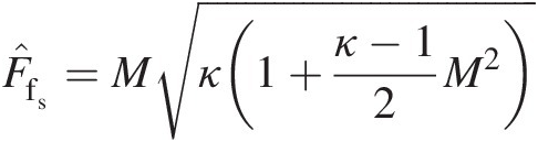
Step 5. Calculate the orifice ideal mass flow rate: ṁideal=ACVF̂fsPsRTt
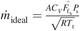
where the velocity coefficient CV = Vx/VCV=Vx/V.
Method 2. This method involves the following calculation steps:
Step 1. Calculate the static temperature: Ts = Tt − V2/2cpTs=Tt−V2/2cp, where V is the total velocity at the orifice exit.
Step 2. Calculate the speed of sound: C=κRTs
Step 3. Calculate the axial-velocity Mach number: Mx = Vx/CMx=Vx/C
Step 4. Calculate the static-pressure mass flow function (see Chapter 2): F̂fs,x=Mxκ1+κ−12Mx2
Step 5. Calculate the orifice ideal mass flow rate: ṁideal=AF̂fs,xPsRTtx
where Ttx=Ts+Vx2/2cp
 .
.


Note that Method 2 can be thought of as Method 1under an inertial transformation where the observer is in a coordinate system that is moving with the velocity Vrθ=V2−Vx2 .
.
4.7 Axial Rotor Thrust
When the gas turbine is stationary, it experiences no axial thrust. The primary flow over compressor and turbine blades and cooling and sealing flows (secondary flows) over disk surfaces generate axial rotor thrust from both pressure forces, which are normal to each surface, and shear forces, which are parallel to each surface. Generally, the contribution of shear forces to axial rotor thrust is negligible compared to the contribution from pressure forces. If the rotor surface is along the axial direction, it makes no contribution to axial thrust. Also the pressure distribution in a closed rotor cavity does not contribute to rotor thrust. An accurate calculation of the rotor thrust is critical to the design of the rotor thrust bearing, which plays an important role in ensuring engine operational and structural integrity.
Because compressor main flow occurs under an adverse pressure gradient (pressure increases in the flow direction), the compressor rotor thrust points in the negative flow direction; we call it the forward thrust. In the turbine flowpath, the pressure decreases downstream, causing the rotor thrust in the flow direction; we call it the rearward or aft thrust. Because compressor and turbine are commonly mounted on the same shaft, the net rotor thrust, which the thrust bearing has to withstand, is always lower than the individual contribution either from the compressor or turbine.
4.7.1 Computation of Axial Thrust on Blades
If we know the distribution of static pressure over a rotor surface, for example, from a 3-D CFD analysis, the axial thrust is simply the axial component of the pressure force integrated over the entire rotor surface. In view of both the complex surface geometry and static pressure distribution, the compressor and turbine rotor thrust calculations can be a tedious undertaking. A design-friendly approach to calculate the axial thrust on blades in each compressor stage or turbine stage is by using a large control volume analysis of the linear momentum equation in the axial direction. Such a control volume is shown in Figure 4.23a as ABCD. To further simplify the momentum analysis, we invoke the concept of stream thrust, which is the sum of the inertia force and pressure force at a section, presented in Chapter 2. If STinSTin is the total stream thrust at inlet AB of the control volume ABCD and SToutSTout the total stream thrust at its outlet CD, we can write
where FbladesFblades and Fca sin gFcasing are the forces from the blades and casing, respectively, assumed to be acting on the fluid control volume in the flow direction. We compute Fca sin gFcasing as the product of the average pressure in the blade tip clearance and the projected casing surface area that is normal to the axial direction. If the casing is diverging along the flow direction, Fca sin gFcasing is positive, and it is negative for a converging casing. The axial aerodynamic load F˜blades on the blades is the reaction force of FbladesFblades, giving F˜blades=−Fblades
 . Thus, Equation 4.58 yields
 (4.59)
Figure 4.23 (a) Schematic of blade and rotor disk for axial thrust calculation and (b) linear variation of static pressure on the axial projection of an axisymmetric compressor or turbine rotor surface element spanning from r1r1 to r2r2.
An accurate calculation of STinSTin and SToutSTout requires a 3-D CFD analysis of the main flow path. We can postprocess the detailed CFD results to compute STinSTin along AB and SToutSTout along CD of the annulus. An alternate method to compute STinSTin and SToutSTout uses the results of a throughflow analysis using circumferentially-averaged flows through multiple stream tubes in the main flow annulus, as for example, presented by Oates (1988). In this case, both at inlet and outlet, we simply sum the stream thrust associated with each stream tube.
4.7.2 Computation of Axial Thrust on Rotor Disks
Axial thrust on the compressor and turbine rotor structure in contact with internal flows (secondary flows) used for cooling and sealing is determined almost entirely by the neighboring vortex structure. We, therefore, first establish the generalized vortex distribution in the rotor-rotor and rotor-stator cavities using the methodology presented in Section 4.3. Using the radial equilibrium equation, we can compute the static pressure at each radial location on the rotor disk. We can also obtain the static pressure distribution on the rotor disk surfaces from a 3-D CFD analysis in the cavities on both forward and rearward (aft) sides. As shown in Figure 4.23a, we use a piece-wise linear distribution of the static pressure along the nodal representation of the axisymmetric rotor disk surfaces. Note that any three-dimensional protrusion, like bolts, on the disk will have negligible additional axial thrust contribution. Between any two nodes on the disk, one can compute the axial thrust contribution either by assuming an average static pressure between the nodes or using a linear variation of static pressure between them.
For the rotor surface element shown in Figure 4.23b, the axial thrust using the average static pressure is computed by
 (4.60)
The linear variation of static pressure on the rotor surface can be expressed by the equation
where A = (Ps2 − Ps1)/(r2 − r1)A=(Ps2−Ps1)/r2−r1 and B = Ps1 − Ar1B=Ps1−Ar1. Using this linear profile equation, the elemental axial thrust can be computed as
 (4.62)
Because the axisymmetric rotor surface area varies as square of the radius, the rotor thrust calculated by Equation 4.62 is more accurate than that by Equation 4.60. The difference is given by
 (4.63)
Because any complex variation in either the rotor surface geometry or the surface pressure can be accurately represented by a piece-wise linear variation, the assumption of the linear pressure variation is not limiting. Equation 4.62, therefore, provides an accurate building block for the calculation of rotor thrust, which can be finally expressed for each rotor in the positive axial direction as
 (4.64)
4.8 Concluding Remarks
We have presented in this chapter some unique thermofluids concepts that are at the heart of designing gas turbine internal flows and their 1-D modeling. These concepts include generalized vortex structure in rotor-stator and rotor-rotor cavities, windage, and induced rotor disk pumping flow for which a simple physics-based argument is presented to determine its direction (radially inward or outward) in the disk boundary layer (Ekman layer) based on the swirl factor of the adjacent vortex core outside the boundary layer. The discussion of the centrifugally-driven buoyant convection in compressor rotor cavities, with and without the bore flow, highlights the nonequilibrium and complex flow and heat transfer physics present in these cavities. However, a simplified 1-D heat transfer modeling methodology for these cavities is presented for design implementation and continuous product validation. The case without the bore flow is treated like a closed rotor cavity. We also presented in this chapter a design-oriented methodology to compute windage and swirl distributions in a purged rotor cavity formed by surfaces with arbitrary rotation, counter-rotation, and no rotation.
Hot gas ingestion and rim seals currently remain the areas of most active research. In a gas turbine design, the objective of any reduction in the flow through a rim-seal to prevent hot gas ingestion must be weighed against the competing increase in the windage temperature rise in the wheel-space. Both the single- and multiple-orifice models for hot gas ingestion presented here will provide the validation flexibility and modeling simplicity necessary to develop an effective rim-seal design in gas turbines.
The preswirl system, while it helps to reduce the temperature of the blade cooling air, must simultaneously ensure that the supply pressure at the blade root is adequate to provide an acceptable backflow margin for the film cooling holes.
We have also presented in this chapter a method to calculate the rotor axial thrust, the accuracy of which depends on the accuracy of the pressure force, which is to be determined from the static pressure distribution (in the generalized vortex core) integrated with area over each disk face.
Worked Examples
Example 4.1
In Section 4.3, for a rotor-stator cavity, we formulated the calculation of windage power and the related change in fluid total temperature in an inertial reference frame. This formulation essentially uses the angular momentum and windage equations as follows:
Angular momentum equation: ΓR−ΓS=ṁrout2SfoutΩ−ṁrin2SfinΩ
Windage equation: TtSout−TtSin=ΓRΩṁcp


After replacing the rotor torque ΓRΓR by the stator torque ΓSΓS from the angular momentum equation, express the windage equation in terms of total temperatures in the rotor reference frame and interpret the terms in the resulting equation.
Solution
Using the angular momentum equation to substitute for ΓRΓR in the windage equation, we obtain


which is the windage equation in terms of rothalpy where IinIin and IoutIout are the fluid rothalpy at the cavity inlet and outlet, respectively. This equation shows that the increase in rothalpy outflow over its inflow equals ΓSΩΓSΩ, as if the stator becomes a rotor in the rotor reference frame and imparts the equivalent windage power to the fluid. When the stator torque is zero, implying an all-rotor cavity, the fluid rothalpy remains constant for an adiabatic flow, which is consistent with the Euler’s turbomachinery equation presented in Chapter 2.
In the aforementioned windage equation, expressing IinIin and IoutIout in the rotor reference frame by Iin=cpTtRin−rin2Ω2/2 and Iin=cpTtRin−rin2Ω2/2
 , respectively, yields the following windage equation in terms of the total temperature in this reference frame:

This equation shows that the change in relative total temperature as a result of windage consists of two parts. The first part represents the change in the relative total temperature from radius rinrin to routrout in the flow through an adiabatic duct rotating with the angular velocity ΩΩ. The second part is the change in the relative total temperature as a result of work done by an equivalent rotor whose torque equals that of the stator.
Example 4.2
For a small single-stage centrifugal air compressor, schematically shown in Figure 4.24, the key impeller dimensions are rsh = 20 mmrsh=20mm, r1 = 50 mmr1=50mm, and r2 = 75 mmr2=75mm. At Ω = 60000 rpmΩ=60000rpm test speed and inlet air mass flow rate ṁ=1kg/s at Pt1 = 1 barPt1=1bar and Tt1 = 290 KTt1=290K, the compressor discharge occurs at Pt2 = 4.5 barPt2=4.5bar and Tt2 = 524.5 KTt2=524.5K. The slip coefficient at the discharge is 0.94. Assuming that the air in the gap between the stationary casing and impeller, both on forward and aft sides, behaves like a forced vortex with the swirl factor Sf = 0.50Sf=0.50 and constant density corresponding to the compressor discharge conditions, calculate the net axial thrust on the impeller. Neglect the contribution of axial thrust as a result of the change in stream thrust of the impeller flow.

Solution
The radial equilibrium equation for a forced vortex with swirl factor SfSf becomes

which for constant density yields the following radial variation of static pressure in the gap between the impeller and casing

Figure 4.24 shows that the axial thrust exerted by the fluid on surface AB is balanced by the equal and opposite thrust on surface CD. Thus, the net contribution to rotor axial thrust is from the fluid pressure force exerted on surface DE. This rotor thrust is directed to the left and is equal to


In the aforementioned equation to calculate rotor axial thrust, we need to first calculate the values of Ps2Ps2 and ρρ as follows:


Neglecting the contribution of dynamic temperature associated with the flow radial velocity at compressor discharge, we write

From isentropic relations we obtain


and

Thus, the rotor axial thrust can now be calculated as

Problems
4.1 An adiabatic, constant-area pipe is rotating at angular velocity ΩΩ about an axis normal to the pipe axis. For the pipe inlet at r = r1r=r1 and outlet at r = r2r=r2, where rr is the radial distance from the axis of rotation, compute for an air mass flow rate of 1 kg/s1kg/s the change in total pressure and total temperature (in an inertial reference frame) from the pipe inlet to outlet. Neglect any frictional pressure loss in the pipe. How will your answers change if the pipe outlet is closed, resulting in zero mass flow rate?
4.2 In an isentropic forced vortex with constant angular velocity ΩfΩf, show that, between radii r1r1 and r1r1, the change in static temperature equals the change in dynamic pressure associated with the rotational velocity. Thus, the change in total temperature in this vortex equals twice the change in static temperature or the change in dynamic temperature, which is easy to calculate.
4.3 In an isentropic free vortex with constant angular momentum HfHf, show that, between radii r1r1 and r1r1, the change in static temperature is equal and opposite to the change in dynamic temperature associated with the rotational velocity. Thus, the total temperature in this vortex remains constant everywhere.
4.4 In some gas turbines, radial pipes are used in the compressor rotor cavity to bring a part of the compressor primary air flow from rim to bore for downstream cooling of turbine parts. One such design is schematically shown in Figure 4.25. The primary design intent is to have the coolant air at location A with a minimum drop in pressure from its value at the extraction point. For this design, the following representative data are given:
PtS = 5 barPtS=5bar; TtS = 500 KTtS=500K; ṁ=10kg/s ; Ω = 3600 rpmΩ=3600rpm
Number of radial pipes = 20
Pipe ID = 40 mm40mm; Pipe OD = 45 mm45mm; L = 1 mL=1m; r1 = 0.15 mr1=0.15m; r2 = 0.2 mr2=0.2m; Darcy friction factor f = 0.022f=0.022.
Note that the compressor air enters each pipe in solid-body rotation with the rotor (Sf = 1.0Sf=1.0), and the flow is assumed to be adiabatic.
Compute at location A:
(a) Static pressure and the corresponding total pressure in both stator and rotor reference frames.
(b) Total temperature in both stator and rotor reference frames.
(c) Air swirl factor.

Figure 4.25 Schematic of a compressor rotor cavity with radial pipes for supplying compressor air for downstream cooling of turbine parts (Problem 4.4).
4.5 Figure 4.26 schematically shows radially inward flow of air in a compressor rotor cavity extracted for downstream cooling of turbine parts. If one assumes that the cooling air reaches the bore region via a free vortex, its static pressure will drop significantly – an undesirable outcome that may result in some backflow. Fortunately, the air that enters the rim region flows radially inward in the Ekman boundary layers on the rotor surface. In general, as shown in the figure, the total mass flow rate ṁ splits into two unequal mass flow rates ṁ1
 and ṁ2
 , where ṁ1
 is for the flow along the left-hand side rotor surface, and ṁ2
 along the right-hand side rotor surface.

Figure 4.26 Schematic of radially inward flow of air in a compressor rotor cavity extracted from the primary flow for downstream cooling of turbine parts (Problem 4.5).
The coordinates of nodes for a piece-wise linear profile of the axisymmetric compressor rotor surface shown in Figure 4.26 are given as follows:
| Node | x (m)xm | r (m)rm |
|---|---|---|
| 1 | 1.90 | 0.25 |
| 2 | 2.10 | 0.40 |
| 3 | 2.10 | 1.05 |
| 4 | 2.00 | 1.20 |
| 5 | 1.05 | 1.20 |
| 6 | 0.90 | 1.05 |
| 7 | 0.90 | 0.30 |
| 8 | 1.10 | 0.15 |
| 9 | 1.90 | 0.15 |
The compressor rotor cavity rotates at Ω = 3600 rpmΩ=3600rpm. The coolant air enters the cavity at the rim at PtS = 5 barPtS=5bar, TtS = 500 KTtS=500K, at a mass flow rate of ṁ=10kg/s . Using multiple control volumes, which may be refined from the ones shown in the figure, along each rotor surface and carrying out the torque (based on empirical correlations presented in this chapter) and angular momentum balance in each control volume, compute ṁ1
 , ṁ2
, ṁ2 , and the common static pressure at the location in the bore region where the two flows join together.
4.6 Repeat the axial thrust calculation of Example 4.1 for a centrifugal air compressor, assuming the swirl factor of 0.45 between the casing and impeller and treating the forced vortex as isentropic.
4.7 A design tool, such as developed under Project 4.1, to compute the distribution of windage and swirl velocity in a general rotor cavity is hardwired for air as the working fluid. Develop a set of scaling equations to convert the results obtained from this design tool to be applicable for another working fluid with known thermophysical properties.
4.8 What role does the windage heating in a wheel space cavity play in the turbine rim seal design for maximum sealing effectiveness while minimizing the sealing air flow rate?
4.9 Repeat the calculations of Example 4.2 under both isentropic and isothermal assumptions for the forced vortex (see Chapter 2) in the gaps between the impeller and casing. Assume that the static pressure and temperature obtained in Example 4.2 at the impeller exit prevail at the gap outer radius. Compare and comment on the rotor axial thrust values obtained under different forced vortex assumptions.
4.10 Assuming that the centrifugal compressor in Example 2.4 discharges radially with no axial velocity, compute the contribution to rotor axial thrust from the given flow through the compressor. Will it increase of decrease the rotor axial thrust calculated in this example?
Projects
4.1 Develop a general purpose stand-alone computer code in FORTRAN, or the language of your choice, to solve for swirl distribution and total temperature change as a result of windage in a general rotor-stator cavity, which is schematically shown in Figure 4.8. For calculating the torque of stator and rotor surfaces in the angular momentum equation, you may use the empirical equations presented in this chapter or others of your preference. For solving the resulting transcendental equation to find the fluid swirl factor in each cavity control volume, you may use the regula falsi routine listed in Appendix D. Assume that all the cavity surfaces are adiabatic. How will you verify your computer code, and how will you validate it?
4.2 Develop a general purpose stand-alone computer code in FORTRAN, or the language of your choice, for handing hot gas ingestion using the multiorifice spoke model presented in Section 4.6.2.2 and schematically shown in Figure 4.22. For the numerical solution of the two-point boundary value problem for each spoke represented by serially-connected orifices, use the Thomas Algorithm presented in Appendix E.
4.3 In the rim seal design shown in Figure 4.20 and the corresponding multispoke model shown in Figure 4.22, we have assumed that the flow happens in each spoke in the meridional plane only, with no spoke-to-spoke interactions in the tangential direction. To include such interactions we can easily extend the spoke model into a fan model for which the grid system in the meridional-tangential plane is shown in Figure 4.27a and the corresponding flow network model in Figure 4.27b. In this project, you are asked to extend the computer code developed under Project 4.2 to solve for various flow properties in the network shown in Figure 4.27b. The problem is akin to 2-D numerical heat conduction solution requiring row-by-row solution using TDMA first in the meridional direction followed by column-by-column TDMA-based solution in the tangential direction until convergence.

Figure 4.27 (a) Grid system for the multiorifice fan model in the meridional-tangential plane and (b) Flow network representation of multiorifice fan model for hot gas ingestion simulation (Project 4.3).
References
Bibliography
Nomenclature
- A
Area
- Âgap

Seal area per vane (Âgap=Agap/N
 )
)
- b
Width of bolt head
- cpcp
Specific heat at constant pressure
- C
Speed of sound
- CdCd
Discharge coefficient
- CDCD
Drag coefficient
- CfCf
Shear coefficient
- CMCM
Moment coefficient
- CVCV
Velocity coefficient (CV = Vx/VCV=Vx/V)
- CV
Control volume
- CFD
Computational fluid dynamics
- CDBC
Centrifugally-driven buoyant convection
- F
Force
- F̂fs

Dimensionless static-pressure mass flow function
- g
Acceleration as a result of gravity
- G
Ratio of axial clearance to cavity outer radius
- GDBC
Gravitationally-driven buoyant convection
- h
Heat transfer coefficient
- IbIb
Interference factor of adjacent bolts on a disk
- k
Dimensionless cavity static pressure (k=P̂scav
 )
)
- L
Length
- ṁ

Mass flow rate
- M
Mach number
- N
Number of turbine vanes in the primary flow path
- NbNb
Number of bolts
- Nu
Nusselt number
- P
Pressure
- P̂s

Dimensionless static pressure (P̂s=Ps−Psmin/Psmax−Psmin)
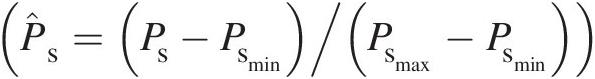
- Pr
Prandtl number
- q̇c

Convective heat flux
- Q̇c

Convective heat transfer rate
- r
Cylindrical polar coordinate r
- R
Gas constant; disk outer radius
- Ra
Rayleigh number
- ReRe
Disk Reynolds number (Re = ρR2Ω/μRe=ρR2Ω/μ)
- Re′Re′
Modified disk Reynolds number (Re′ = ρΩRo(Ro − Ri)/μRe′=ρΩRoRo−Ri/μ
- RRF
Rotor (noninertial) reference frame
- s
Gap between rotor and stator in a cavity; tangential distance between bolds
- SRF
Stator (inertial) reference frame
- t
Time
- SfSf
Swirl factor
- STST
Stream thrust
- T
Temperature
- TawTaw
Adiabatic wall temperature
- U
Rotor tangential velocity
- V
Velocity
- x
Cartesian coordinate x
- x̂

Dimensionless θ coordinate (x̂=Nθ/π−1
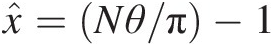 )
)


Subscripts and Superscripts
- 1
Location 1; section 1
- 2
Location 2; section 2
- 3
Location 3; section 3
- 4
Location 4; section 4
- annann
Annulus
- bb
Bolt
- borebore
Compressor bore region
- cavcav
Cavity
- conecone
Conical surface
- cylindercylinder
Cylindrical surface
- disk pumpdiskpump
Disk pumping mass flow rate
- egregr
Egress
- free diskfreedisk
Rotor disk adjacent to stagnant air core
- gapgap
Gap
- hh
Horizontal
- ii
Inner
- inin
Inlet
- inging
Ingress
- maxmax
Maximum value
- minmin
Minimum value
- oo
Outer
- outout
Outlet
- rr
Radial direction
- rθ
In radial-tangential (r − θr−θ) plane
- RR
Rotor; rotor reference frame
- refref
Reference rotor
- ss
Static
- shsh
Shaft
- SS
Stator; stator reference frame
- tt
Total (stagnation)
- ww
Wall
- xx
Axial direction; flow direction
- θθ
Tangential direction
- −

Average

Greek Symbols
- α
Angle of the conical surface from horizontal
- β
Ratio disk angular velocity to reference rotor angular velocity (β = Ω/Ωrefβ=Ω/Ωref)
- ΓΓ
Torque
- ΔΔ
Small change in a quantity
- ζζ
Fraction of free disk pumping mass flow rate
- θθ
Blade cooling air temperature reduction coefficient
- θ˜

Turbine work loss coefficient
- κκ
Ratio of specific heats
- μμ
Dynamic viscosity
- ρρ
Density
- ττ
Shear stress
- ΩΩ
Angular velocity